The role of submesoscale filaments in restratification of the surface mixed layer and dissolved oxygen variability in large Lake Geneva: field evidence complemented by Lagrangian particle-tracking

1 Introduction

In the Surface Mixed Layer (SML) of oceans and large lakes, submesoscale currents are commonly observed as density fronts, filaments, vortices and topographic wakes with a lateral scale of O(0.1-10 km) and a timescale of hours to days (McWilliams, 2019). They are characterized by the bulk Richardson number, $R{i}_b=N^2{H}^2/U^2$ and Rossby number, $R{o}_b=U/fL$, both of O(1) (Thomas et al., 2008; Bracco et al., 2019; Yu et al., 2019; Chrysagi et al., 2021), with U being the characteristic speed, H the vertical length scale, L the horizontal length scale of the velocity field, N the buoyancy frequency and f the Coriolis parameter. The existence of submesoscale flows was first revealed by remote sensing imagery in the 1980s (McWilliams, 1985; D’Asaro, 1988), but their dynamics and impact remain poorly understood (Lévy et al., 2018; Kaiser et al., 2021). Although a diverse array of well-established field measurement tools, such as ship-towed devices (e.g., SeaSoar (Pidcock et al., 2010; Triaux (D’Asaro et al., 2011); SMILES (Adams et al., 2017)), the underway CTD (Rudnick and Klinke, 2007), or the ecoCTD (e.g., Dever et al., 2020), nested clusters of mooring arrays (OSMOSIS (Yu et al., 2019), SubMESI (Zhang Z. et al., 2021), and autonomous underwater vehicles (e.g., Carpenter et al., 2020; Salm et al., 2023), have been employed to investigate submesoscale dynamics in ocean studies, obtaining in situ evidence for fine-scale submesoscale dynamics, such as filaments with a horizontal scale ranging from O(10 m) to O(100 m), remains challenging due to the ephemeral nature of submesoscale flows and their spatial heterogeneity (Lévy et al., 2018; Kock et al., 2023). With increasing computational capacity, numerical models with higher resolution have led to a better understanding of their dynamics (Klein and Lapeyre, 2009; Zhong and Bracco, 2013; Bracco et al., 2019), revealing a plethora of submesoscale flows coexisting with mesoscale circulations and exhibiting strong horizontal and vertical velocities in pelagic (offshore) zones (Klein et al., 2008; Brannigan, 2016; Chrysagi et al., 2021). About half of the variance in vertical velocities in the upper layer of the ocean is attributed to submesoscale processes (Klein and Lapeyre, 2009).

Submesoscale filaments, which are typically observed as elongated patches at different temperatures/densities within mesoscale rotational motions (e.g., gyres and eddies; Hamze-Ziabari et al., 2022a), are the focus of this study. Submesoscale filaments are formed as a result of the rapid sharpening of a density gradient by horizontal deformation flows, a process known as filamentary intensification (McWilliams et al., 2009) or filamentogenesis (Gula et al., 2014). During this process, dual frontogenesis causes the convergence of two overturning cells with stronger surface convergence and downwelling at the center of the cold filament, which restores geostrophic balances and re-stratifies the SML. Due to the vertical motion associated with submesoscale processes, momentum and tracers such as heat, mass, oxygen, pollutants and carbon can be exchanged between the surface and the deep pycnocline (Smith et al., 2016; Erickson and Thompson, 2018; Su et al., 2018; Archer et al., 2020; Freilich and Mahadevan, 2021).

Existing observational evidence and numerical studies indicate that submesoscale processes such as fronts and filaments can play an important role in ocean productivity, biogeochemical fluxes and biodiversity patterns (Mahadevan, 2016; Pascual et al., 2017; Lehahn et al., 2018; Hernández-Hernández et al., 2020; Fadeev et al., 2021; Kaiser et al., 2021; Campanero et al., 2022; Xiu et al., 2022). Based on an idealized modeling study, Lévy and Martin (2013) demonstrated that the primary production associated with mesoscale currents can be underestimated by a third if submesoscale processes are not included. The spatial variability of biogeochemical parameters observed in submesoscale fronts or filaments can be explained by three mechanisms: active, passive and reactive (Lévy et al., 2018). In the passive mechanism, small-scale filamentary patches of preexisting phytoplankton are formed by stirring and deformation associated with mesoscale processes (Birch et al., 2008; Demarcq et al., 2012). During the active phase, vertical motions associated with filamentogenesis/frontogenesis are responsible for transporting nutrients from the deep nutricline into the euphotic zone (Ramachandran et al., 2014) and lead to small patches of phytoplankton bloom in frontal or filamentary zones (Lévy et al., 2001; Mouriño et al., 2004; Lehahn et al., 2007; Mangolte et al., 2022). The reactive mechanism is related to phytoplankton reactions to the active and passive mechanisms, which include competition, swimming, mortality, deposition and grazing by herbivores (e.g., zooplankton) (Flierl and Woods, 2015; Lévy et al., 2018; Taylor, 2018). Such intricate processes associated with submesoscale dynamics require high-resolution comprehensive numerical and observational evidence in order to be fully understood.

Traditionally, processes affecting density stratification in the upper part of a lake have been studied only from a vertical perspective and the SML is generally considered to be well-mixed (Chrysagi et al., 2021). However, the contribution of lateral processes, such as submesoscale instabilities, to the thermal stratification of lakes has been neglected. Sharp lateral density gradients due to the presence of filaments/fronts make the SML susceptible to different kinds of instabilities such as mixed-layer baroclinic (Boccaletti et al., 2007), gravitational, symmetric (Thomas et al., 2013) and inertial/centrifugal instabilities (Grisouard, 2018). Theoretical and numerical studies showed that submesoscale instabilities are rapidly evolving features that enhance vertical exchange and tend to re-stratify the ocean’s SML (Couvelard et al., 2015; Chrysagi et al., 2021; Jiang et al., 2022).

Recent studies using high-resolution satellite imagery, numerical models and field observations revealed that the SML dynamics in lakes can also be characterized by submesoscale filaments and fronts (Foroughan et al., 2022; Hamze-Ziabari et al., 2022b). Hamze-Ziabari et al. (2022a) reported that submesoscale filaments are formed in Lake Geneva, the largest freshwater lake in Western Europe, during the strongly stratified summer season, and that they are likely ubiquitous features of quasi-geostrophic gyres in large lakes. Foroughan et al. (2022) also employed a combination of field observations, numerical modeling, and satellite images to document a persistent submesoscale frontal slick in Lake Geneva. Field evidence in Lake Geneva suggested that submesoscale filaments/fronts can potentially impact on the mixing of the water column, when the thermocline is in close proximity to the surface layer (Hamze-Ziabari et al., 2022a). Furthermore, a procedure was developed by Hamze-Ziabari et al. (2022c); Hamze-Ziabari et al. (2023) to detect mesoscale and submesoscale gyres/eddies and their associated pelagic upwelling/downwelling in Lake Geneva. The procedure can be applied to predict when and where regularly-occurring gyre patterns and associated submesoscale filaments are expected to form and thus allows capturing them in field measurements.

To our knowledge, the potential impact of submesoscale filaments on mixed layer stratification and biological processes in lakes has, thus far, not been investigated. Therefore, the objective of the present study is to provide direct field evidence of Surface Mixed Layer (SML) re-stratification with a horizontal resolution of O(1 m) under fall and winter conditions when lake thermal stratification is weak and the SML is deep. Based on the predictive procedure we developed, two ship-towed field campaigns were designed and carried out in 2020 to investigate cold filaments originating from both coastal and pelagic (offshore) upwelling under complex multi-scale rotational flow fields. Two additional field campaigns were designed and carried out in 2021 to explore the spatial variability of Dissolved Oxygen (DO) near the cold filaments under weakly stratified conditions. These field observations were combined with numerical simulations and particle tracking. In a novel approach, Lagrangian particle tracking is employed to investigate the dynamics of the secondary circulation associated with submesoscale filaments and how it is linked to the re-stratification within adjacent water columns. The present study aims to gain insight into the spatial variability of stratification strength, vertical velocities, and the distribution of DO influenced by secondary circulation dynamics in the vicinity of cold filaments. Although this study was carried out in a large lake, the results on filament dynamics can be directly applied to oceans, where obtaining field evidence with equivalent spatial resolution presents significant challenges.

2 Materials and methods

2.1 Study site

Often referred to as the birthplace of limnology (Forel, 1892), Lake Geneva (local name: Lac Léman) is the largest lake in Western Europe. It is a crescent-shaped water body located between Switzerland and France. Lake Geneva is composed of two basins: a narrow western basin called the Petit Lac, with a maximum depth of 75 m, and a large eastern basin, the Grand Lac, with a mean depth of 170 m and a maximum depth of 309 m, with a total volume of approximately 89 km³ and a mean surface altitude of 372 m. It is a peri-alpine, warm monomictic lake with a strong thermal stratification during the summer. The thermocline deepens during fall and winter but typically does not disappear entirely. Due to the relatively large size of Lake Geneva, Coriolis force effects contribute significantly to the momentum balance, as was documented in numerous field observations and numerical studies (e.g., Bauer et al., 1981; Lemmin et al., 2005; Bouffard and Lemmin, 2013; Cimatoribus et al., 2018; Cimatoribus et al., 2019; Lemmin, 2020; Reiss et al., 2020; Hamze-Ziabari et al., 2022c; Reiss et al., 2022).

The topography surrounding the lake, in particular, the Jura and Alp mountains, channels two strong pressure-gradient winds which are called the Vent, blowing from the southwest, and the Bise, from the northeast over most of the lake surface (Figure 1A). These winds are generally uniform in space and last for several days, with speeds averaging between 5 and 15 m s⁻¹ (e.g., Lemmin and D’Adamo, 1996; Lemmin et al., 2005). The Vent and Bise winds are therefore the primary external forcing for the initiation of multiscale rotational flow fields (gyres and eddies; both cyclonic and anticyclonic). Their interaction with lake bathymetry and shore morphology creates a “soup” of gyres, eddies, fronts and filaments (Hamze-Ziabari et al., 2022c).

FIGURE 1

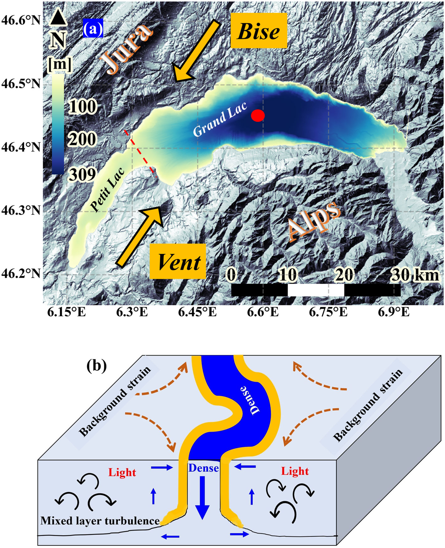
Figure 1 (A) Lake Geneva and surrounding topography, adapted from a public domain satellite image (NASA World Wind, last accessed 31 December 2022) and bathymetry data from SwissTopo (last accessed 31 December 2022). The red dashed line delimits the two basins called Petit Lac and Grand Lac that compose Lake Geneva. Red circle: location of the SHL2 station, a long-term CIPEL monitoring station where physical and biological parameters are regularly measured. The thick orange arrows indicate the direction of the two strong dominant winds channeled by the Alp and Jura mountains, namely the Bise, coming from the northeast and the Vent, from the southwest. The colorbar gives the water depth. (B) Sketch of filamentogenesis, i.e., dual frontogenesis, caused by large-scale deformation flow on a dense filament (winding blue band) located in the “light” (lower density) Surface Mixed Layer (SML). Small blue arrows: secondary circulation associated with dense filaments. Yellow borders: areas susceptible to submesoscale instabilities.

2.2 Hydrodynamic model

We employed the MITgcm code, which integrates the three-dimensional (3D) Reynolds-Averaged Navier-Stokes (RANS) equations on a sphere under the Boussinesq and both hydrostatic and non-hydrostatic approximations (Marshall et al., 1997). Originally developed for oceanography, the code has also been successfully applied to lakes (Dorostkar and Boegman, 2013; Djoumna et al., 2014; Dorostkar et al., 2017). Prior to the present study, the model was calibrated for Lake Geneva and accurately reproduced seasonal thermal stratification, mean flow field and internal seiches (Cimatoribus et al., 2019), nearshore currents, coastal upwelling, inter-basin exchange and river plume dynamics (Cimatoribus et al., 2018; Cimatoribus et al., 2019; Reiss et al., 2020; Soulignac et al., 2021; Reiss et al., 2022), basin- and mesoscale rotational flows, as well as submesoscale currents (Foroughan et al., 2022; Hamze-Ziabari et al., 2022a; Hamze-Ziabari et al., 2022b; Hamze-Ziabari et al., 2022c). Here, using the model setup validated by Cimatoribus et al. (2018), the model was run in hydrostatic mode with an implicit free surface.

A high-resolution survey dataset was used to construct Lake Geneva’s bathymetry. Three-dimensional RANS equations were solved for two Cartesian grids with low and high resolution. First, the model was initialized from rest on 3 June 2019 with a Low Resolution (LR) grid (horizontal resolution of 173-260 m and 35 depth layers) based on the measured temperature profile from the Commission Internationale pour la Protection des Eaux du Léman (CIPEL) station SHL2 (center of the lake at a depth of 305 m; Figure 1A) as a horizontally uniform initial condition. The LR model integration time step was 20 s, and spin-up took almost six months in simulation time. Based on the LR model, a High Resolution (HR) version of the model was initialized with a grid resolution of 113 m horizontally and 50 layers vertically; vertical layers have a thickness of 0.30 m at the surface and approximately 12 m at the deepest point. To ensure stability, the time step was initially set to 6 s, then gradually increased to 30 s. HR model simulations began on 10 January 2020 and lasted ten months.

The atmospheric forcing data driving the model was provided by the COnsortium for Small‐scale MOdeling (COSMO) atmospheric model of MeteoSwiss (Voudouri et al., 2017). COSMO produces realistic atmospheric fields (wind, temperature, humidity, solar radiation) applying the bulk formulation of Large and Yeager (2004) to estimate atmospheric exchanges. COSMO data have a 1h time step and 1 km × 1 km spatial resolution.

2.3 Particle tracking

Following fluid particle trajectories allows for the Lagrangian description of a flow field based on the velocity field computed from lake or ocean circulation models. Using 3D numerical simulation results, particle tracking can reveal preferential lateral and vertical transport pathways of fluid parcels. It can also determine the origin (backward tracking) and fate (forward tracking) of material transported via general circulation and driven by meso- to submesoscale currents. In particular, since the number of submesoscale current studies has steadily grown over the past two decades, Lagrangian methods, such as particle tracking, are increasingly being used to evaluate the effect of surface material transport occurring within this scale range (Choi et al., 2017; Freilich and Mahadevan, 2021; Aravind et al., 2023).

This study adopted the particle tracking approach proposed by Döös et al. (2013). Particle trajectories were calculated using linear interpolation between time (between intervals of model outputs) and space (between model grid points), derived from a 3D velocity field generated by a hydrodynamic model. The algorithm is programmed using Python and accepts the MITgcm output format (Cimatoribus et al., 2018). The output trajectories are then verified using the analytical results of Döös et al. (2013). Since the MITgcm hydrodynamic model focuses on deterministic advection by the flow, not on small-scale turbulent mixing, no diffusion of particles is allowed. A further advantage of this method is that it conserves volumes, since the computed trajectories satisfy the no-flow side and bottom boundary conditions. In recent studies, the code was applied to Lake Geneva to investigate the dispersion of the Rhône River, the lake’s primary tributary (Cimatoribus et al., 2019), transport processes during Ekman-type coastal upwelling along the northern shore of the lake that resulted in both vertical and lateral displacements of relatively cold-water masses (Reiss et al., 2020), and inter-basin exchange (Reiss et al., 2022). In the present study, particle tracking is used to estimate the spatial patterns of particle concentration, highlighting the role of submesoscale filaments and the associated secondary circulations in accumulating surface materials and creating vertical pathways for their transport to deeper layers.

2.4 Field measurements

Time series of temperature profiles were measured using a chain of up to 22 temperature loggers (RBRsolo T and Seabird SBE‐56, spaced at 1-2 m intervals and sampling at 1 Hz) towed along a transect, with the horizontal distance between samples depending on the boat’s speed (0.4 - 0.5 m s^-1). This configuration provided a horizontal resolution of ~ 0.5 meters. The average boat speed for each transect is estimated by using GPS data recorded at 10-minute intervals. The boat was stopped three times along each transect to allow a comparison (in post-processing) between the vertical temperature profiles acquired from a vertically suspended chain and an inclined chain. A schematic representation of the estimation of the inclination angle of the chain is given in Figure 2A. A field-based comparison of vertical temperature profiles between the mobile and stationary modes is illustrated in Figure 2B. As shown, the measured temperature profile in the moving mode is effectively corrected by following the procedure outlined in Figure 2A. In total, 17 temperature profiles were assessed using the same method, resulting in a mean absolute error of 0.017°C for the adjusted profiles within the SML. Although this methodology is less accurate than measuring temperature profiles in a stop-start manner, the interpretation of the temperature profiles was not affected. In all cases, the measurements compared reasonably well with the MITgcm simulation results.

FIGURE 2

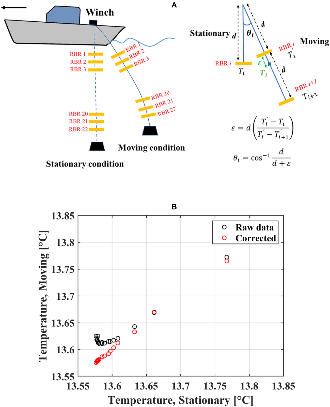
Figure 2 (A) Schematic of the ship-towed temperature measurement set-up and its key components in a typical configuration. ${\theta }_i$ represents the estimated inclination of the chain caused by the boat’s motion. $T_i$ and $T_i^{´}$ denote the temperature readings of RBR solo T temperature logger i under stationary and moving conditions, respectively. d is the distance between two consecutive loggers on the chain (i and i + 1), which is assumed to be the same under stationary and moving conditions. ε is approximated under the assumption of a linear change of temperature between two loggers in the mixed layer depth. The inclination angle of each sensor (${\theta }_i$) was calculated as the arc-cosine of the ratio between the approximated isothermal depth (d+ε) from the inclined chain and the nominal isothermal depth obtained from the vertical chain (d). The chain was ~ 45 m long and the boat moved at 0. 4 - 0.5 m s^-1. (B) A comparison of vertical temperature profiles acquired on October 19, 2020, under both mobile and stationary conditions, along with the temperature adjustments made using the procedure outlined in (A).

A multiparameter probe (CTD90M Sea and Sun Technology) with a PT100 temperature sensor and an optical Dissolved Oxygen (DO) sensor (Rinko III) was used to measure vertical profiles of temperature and DO in a stop-start manner at predefined measurement points along the transects. Following the procedure suggested by Sasano et al. (2011), the Rinko sensor was calibrated for each sampling cast to eliminate biases caused by instrument drift. Velocity profiles were measured continuously with a towed, downward looking (at 0.5 m below the surface) Acoustic Doppler Current Profiler (ADCP); 300kHz Teledyne Marine Workhorse Sentinel in Mode 12 and bottom tracking mode. Current intensities and directions were measured along vertical profiles with 1-m high depth cells, using a profile sampling frequency of 1Hz, resulting in a profile spacing of 0.7–1.4 m along each transect. Manufacturer recommendations were followed for post-processing the measurements.

2.5 Submesoscale instabilities

Sharp lateral density gradients induced by the frontogenesis process make the Surface Mixed Layer (SML) susceptible to different kinds of submesoscale instabilities (Figure 1B), which act on the forward cascade of kinetic energy from mesoscale to dissipation scale (Capet et al., 2008; Brüggemann and Eden, 2015). The interplay between two-celled secondary circulation induced by dual frontogenetic process and different kinds of submesoscale instabilities can lead to re-stratification of the SML (Taylor and Ferrari, 2011; Chrysagi et al., 2021). The different types of submesoscale instabilities are commonly identified based on the signs of Coriolis frequency (f) and Ertel Potential Vorticity (EPV, q), which is defined as (Hoskins, 1974):

$\begin{array}{ll}\mathit{\text{fq}}\mathbf{=}\mathit{\text{f}}\mathbf{(}\mathit{\text{f}}\overrightarrow{\mathit{\text{k}}}\mathbf{+}\mathbf{\nabla }\mathbf{\times }\mathit{\text{u}}\mathbf{)}\mathbf{.}\mathit{\text{∇b}}& (1)\end{array}$

If $fq<0$, various types of instabilities such as inertial (centrifugal), gravitational and symmetric instabilities can occur in the SML (Hoskins, 1974). Since Lake Geneva is situated in the Northern Hemisphere ($f>0$), submesoscale instability occurs when $q<0$. Inertial or centrifugal instability occurs when, under stable stratification ($N^2>0$), the absolute vorticity, ${\xi }_{abs}=f+\xi <0$, is negative (Bachman et al., 2017; Zhurbas et al., 2022). Gravitational instability can occur when N² is negative, i.e., when heavy water parcels are on top of lighter water parcels due to density-driven processes.

In the frontal region, another type of instability known as Symmetric Instability (SI) occurs frequently. In order to detect SI, the EPV is split into a horizontal and a vertical component as follows (Thomas et al., 2013):

$\begin{array}{ll}\mathit{\text{q}}\mathbf{=}{\mathit{\text{q}}}_{\mathit{\text{ver}}}\mathbf{+}{\mathit{\text{q}}}_{\mathit{\text{bc}}}& (2)\end{array}$

$\begin{array}{ll}{\mathit{\text{q}}}_{\mathit{\text{ver}}}\mathbf{=}{\mathit{\text{ξ}}}_{\mathit{\text{abs}}}{\mathit{\text{N}}}^{\mathbf{2}}& (3)\end{array}$

$\begin{array}{ll}{\mathit{\text{q}}}_{\mathit{\text{bc}}}=\left(\frac{\mathbf{\partial }\mathit{\text{u}}}{\mathbf{\partial }\mathit{\text{z}}}\mathbf{-}\frac{\mathbf{\partial }\mathit{\text{w}}}{\mathbf{\partial }\mathit{\text{x}}}\right)\frac{\mathbf{\partial }\mathit{\text{b}}}{\mathbf{\partial }\mathit{\text{y}}}+\left(\frac{\mathbf{\partial }\mathit{\text{w}}}{\mathbf{\partial }\mathit{\text{y}}}\mathbf{-}\frac{\mathbf{\partial }\mathit{\text{v}}}{\mathbf{\partial }\mathit{\text{z}}}\right)\frac{\mathbf{\partial }\mathbf{\text{b}}}{\mathbf{\partial }\mathit{\text{x}}}& (4)\end{array}$

The vertical component ($q_{ver}$) includes the vertical stratification N² and absolute vorticity, ${\xi }_{abs}$, whereas the baroclinic (horizontal) component ($q_{bc}$) is related to the horizontal terms of vorticity and the lateral buoyancy gradients. Symmetric Instability occurs if $f{q}_{bc}\langle 0, \left|f{q}_{bc}\right|\rangle f{q}_{ver}, f{q}_{ver}>0 \text{and } b_z>0$ (Bachman et al., 2017; Zhurbas et al., 2022). The SI can be interpreted as a hybrid gravitational-centrifugal instability that extracts energy from large-scale geostrophic or quasi-geostrophic gyres/eddies. Such slantwise convection can re-stratify the SML and cause a downward cascade of energy through a secondary Kelvin-Helmholtz instability (Taylor and Ferrari, 2009). According to Taylor and Ferrari (2011), frontal regions first become unstable due to SI, and then by baroclinic instability; both tend to increase stratification.

3 Results

After a strong wind event, cyclonic (counterclockwise rotating) and anticyclonic (clockwise rotating) circulations (gyres and eddies) are simultaneously generated in the Grand Lac basin of Lake Geneva (Hamze-Ziabari et al., 2022b). It was shown that the size, location and strength of these patterns can be predicted using the procedure described in Hamze-Ziabari et al. (2022c). Below we will apply this procedure to investigate filament dynamics under weakly stratified conditions. Two different campaigns were carried out: (i) On 19 October 2020, a combination of a larger Anticyclonic Circulation (AC) and a smaller Cyclonic Circulation (CC) was generated in the western part of the Grand Lac. Below, we will analyze the flow field between the two circulations. (ii) On 25 November 2020, Cyclonic Circulation (CC) was predicted in the central part of the Grand Lac with pelagic upwelling in its center. Cold filaments in the center of CC will be investigated. Field data, numerical modeling results and particle tracking will be combined in the analysis.

3.1 Field campaigns based on numerical modeling predictions

3.1.1 Cold filaments at the periphery of large-scale circulations

On 19 October 2020, the numerical model predicted the formation of submesoscale cold filaments near the periphery of both CC and AC (Figure 3A). Therefore, a field campaign was conducted to capture both mesoscale and submesoscale processes associated with AC and CC. The chain of temperature loggers and the ADCP were towed along transect T1 (Figure 3A) which was preselected before the start of the campaign based on the forecast of the numerical modeling. The resultant temperature pattern (Figure 3B) shows that the AC flow field is associated with warm zones in the northern part of the lake, whereas the CC flow field is associated with cold zones in the southern part. This spatial temperature variability can be attributed to pelagic upwelling generated by the CC, and pelagic downwelling, by the AC. The numerical model also predicts reasonably well this spatial temperature variability (Figure 3C).

FIGURE 3

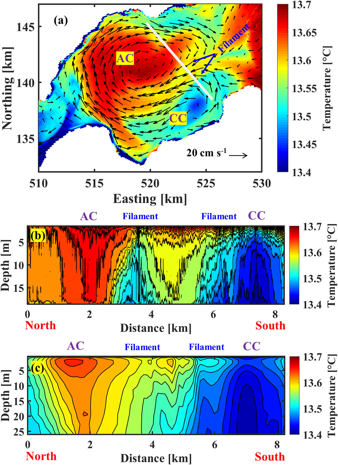
Figure 3 For 19 October 2020: (A) Numerical results for the temperature (colors) and velocity (black arrows; see reference arrow) fields at 1-m depth, showing an Anticyclonic Circulation (AC) in the north and a Cyclonic Circulation (CC) in the south, in the western part of the Grand Lac basin of Lake Geneva. The grey line marks the predefined transect T1 for the field campaign. The location of the filaments is indicated. Contour plots based on (B) measured and (C) simulated temperature profiles along transect T1 shown in (A) Colorbars give the temperature range. Note that the temperature range is identical in (B, C).

At the peripheries of CC and AC, two cold filaments formed, as seen in the numerical modeling results (arrows in Figure 3A). Field results confirm the presence of two narrow cold regions with ~1 km width inside the CC and AC fields. Based on the numerical results (Figures 4A, B), Rossby and Richardson numbers are both O(1) in the SML, indicating that the cold filamentary regions can be classified as submesoscale flows. The averaged divergence and horizontal strain rate parameters over the SML are presented in Figures 4C, D, respectively. The divergence, σ, and horizontal strain rate, S, parameters are given by:

FIGURE 4

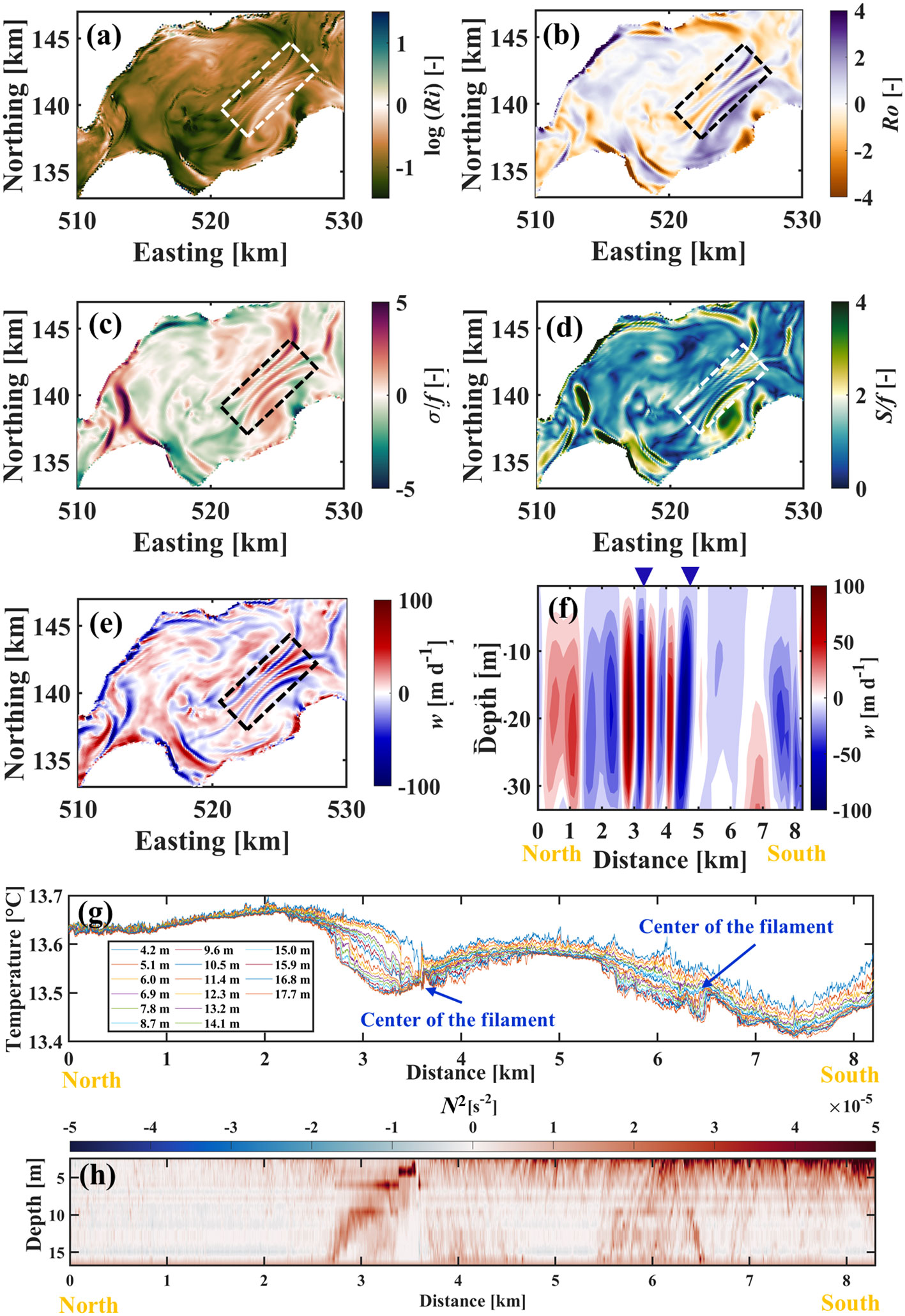
Figure 4 Results from the high-resolution, 3D numerical simulation at 5-m depth for 19 October 2020 in the western part of the Grand Lac basin: (A) balanced Richardson number, Ri, (B) local Rossby number, Ro, (C) normalized divergence parameter, σ/f, (D) normalized horizontal strain rate, S/f; f is the Coriolis frequency, (E) vertical velocity, w. The dashed lined rectangles in (A–E) mark the location of the cold filaments in Figure 3. (F) Vertical profiles of w along transect T1 shown in Figure 3A. Blue triangles on top of the panel indicate the location of the filaments. (G) Measured temperature along transect T1 at different depth layers in the SML. (H) Estimated stratification strength, N², based on the measured temperature profiles along transect T1. The legends give the range of the parameters.

$\begin{array}{ll}\mathit{\text{σ}}\mathbf{=}{\mathit{\text{u}}}_{\mathit{\text{x}}}\mathbf{+}{\mathit{\text{v}}}_{\mathit{\text{y}}}& (5)\end{array}$

$\begin{array}{ll}\mathit{\text{S}}\mathbf{=}\sqrt{{({\mathit{\text{u}}}_{\mathit{\text{x}}}\mathbf{-}{\mathit{\text{v}}}_{\mathit{\text{y}}})}^2\mathbf{+}{({\mathit{\text{v}}}_{\mathit{\text{x}}}\mathbf{+}{\mathit{\text{u}}}_{\mathit{\text{y}}})}^2}& (6)\end{array}$

High divergence/convergence zones are accompanied by high (submesoscale) horizontal strain rates (> f) within the filament and adjacent cells. The presence of large-scale straining flows (e.g., AC and CC) and lateral buoyancy gradients can lead to frontogenesis or filamentogenesis (Gula et al., 2014; McWilliams et al., 2015; Hamze-Ziabari et al., 2022a). Secondary circulation is therefore expected to occur. The numerical results also reveal strong vertical velocities (100 m d^-1) in the center (Figure 4E) and in the vicinity of the observed cold filaments (Figure 4F). Dual frontogenetic processes involved in filamentogenesis result in downwelling at the center of the filament and upwelling in the areas adjacent to the cold filaments (McWilliams et al., 2009). The upward velocities around the cold filaments and the downward velocities inside the cold filaments are indicative of the secondary circulation, which tends to dynamically collapse vertical isotherms towards horizontal isotherms, thereby re-stratifying the SML.

The measured temperature obtained by the towed thermistor node chain at different depth layers (Figure 4G) and the stratification strength ($N^2,$Figure 4H) along transect T1 (Figure 3A) show the enhancement of stratification on both sides of the cold filament in the SML, particularly in the range of 2.5-3.5 km where the temperature gradient between the cold filament and AC is more pronounced. In the non-frontal regions, N² is negligible. However, it can reach 5 × 10^-5 s^-2 in the SML (down to 17-m depth; Figure 4H) in areas next to the filament. The frontal region formed between AC and CC shows an increase in stratification strength between 5.5-6.5 km. The high stratification strength in the near-surface layers is primarily due to warming that occurred during the field campaign (10:25 to 14:53 CET). More details about the atmospheric conditions during the field campaign are given in the Discussion section.

3.1.2 Cold filaments in the center of a cyclonic circulation

On 25 November 2020, the numerical modeling predicted a cyclonic gyre (CC) in the center of the Grand Lac basin (Figure 5A). Cyclonic gyres can produce pelagic upwelling at their centers and thereby provide the buoyancy gradient for the formation of submesoscale filaments and fronts in the pelagic zone of large lakes (Hamze-Ziabari et al., 2022b). From the modeling results, two transects, T2 and T3, were preselected to capture the frontal or filamentous regions associated with pelagic upwelling. The temperature profiles measured along transects T2 and T3 are given in Figures 5B, D, respectively. Intense pelagic upwelling in the center of the cyclonic gyre is clearly visible in the thermocline layer in transect T3, which is closer to the center of the cyclonic gyre (Figure 5A). The upwelled thermocline is not as evident in transect T2 since it is located at the edge of the gyre. A narrow cold region with ~500 m width can be observed in the SML of T2 (Figure 5C). A frontal region between the center of the cyclonic gyre and the edge of the gyre was formed due to intense pelagic upwelling (Figure 5D). Interestingly, there is a narrow cold region of ~200-m width at a distance of ~2.7 km in the boundary of the front (Figure 5E).

FIGURE 5

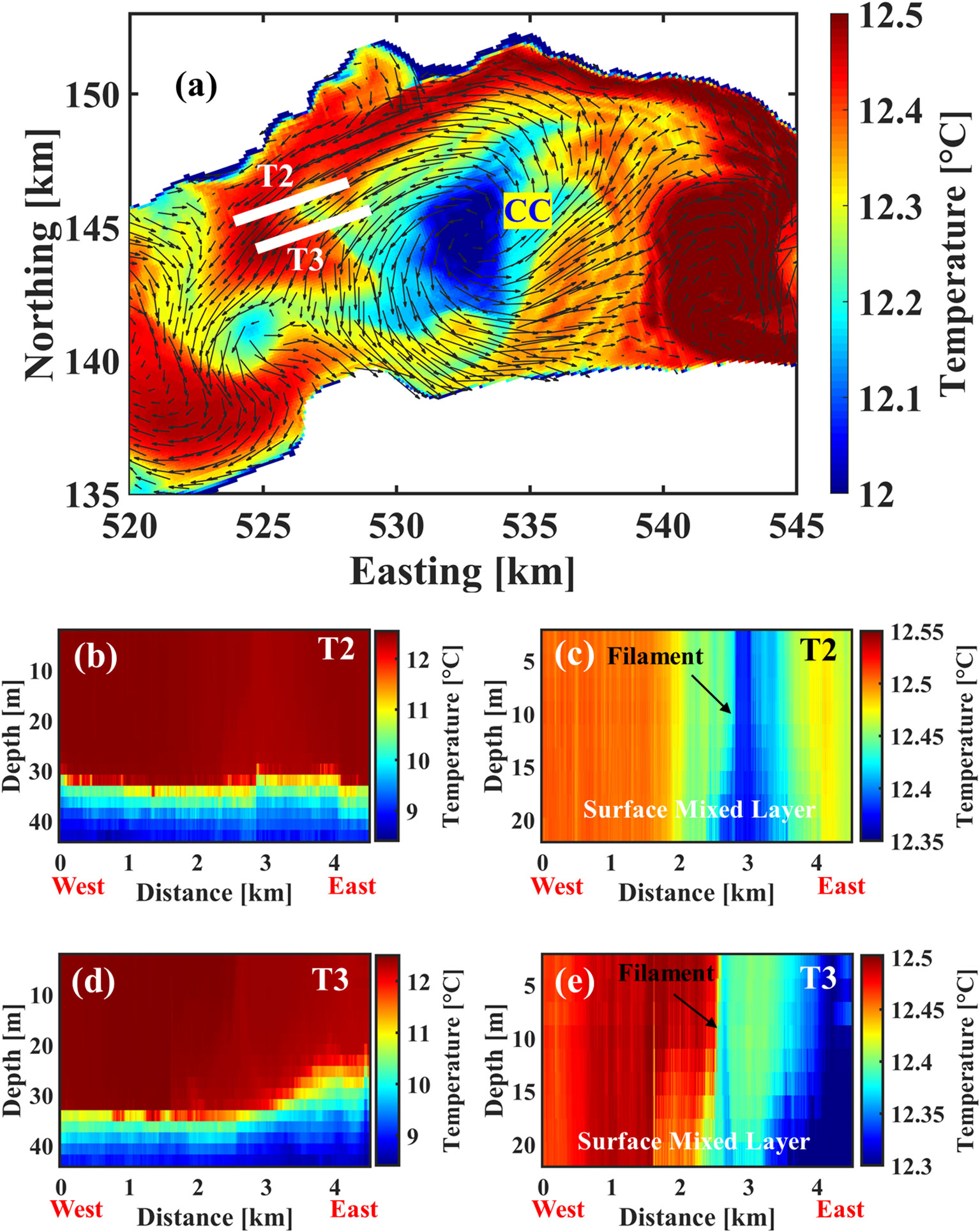
Figure 5 For 25 November 2020: (A) Modeled temperature (colors) and velocity (black arrows; see reference arrow) fields at 1-m depth showing a cyclonic circulation (CC) in the central part of the Grand Lac. Grey lines mark predefined transects (T2 and T3) for the field campaign. Measured profiles of temperature (B) over a 45-m depth range and (C) in the surface mixed layer along transect T2 shown in (A). Measured profiles of temperature (D) over a 45-m depth range and (E) in the surface mixed layer along transect T3 shown in (A). Colorbars give the temperature range.

The vertical profiles of the simulated temperature, vertical velocity, horizontal strain and divergence parameters are given in Figure 6. At the location of the cold filament, strong downwelling velocities, reaching ~100-150 m d^-1, are observed in the center of the cold filament. Strong convergence ($\sigma <-f$) and strain ($S>f$) are accompanied by strong vertical velocities at the center of the cold filament (Figure 6). Vertical velocities, divergence, and strain parameters are confined to the SML, limited by the thermocline layer, which acts as a physical barrier. The presence of secondary circulation is evident in transects T2 and T3 (Figures 6B, F).

FIGURE 6

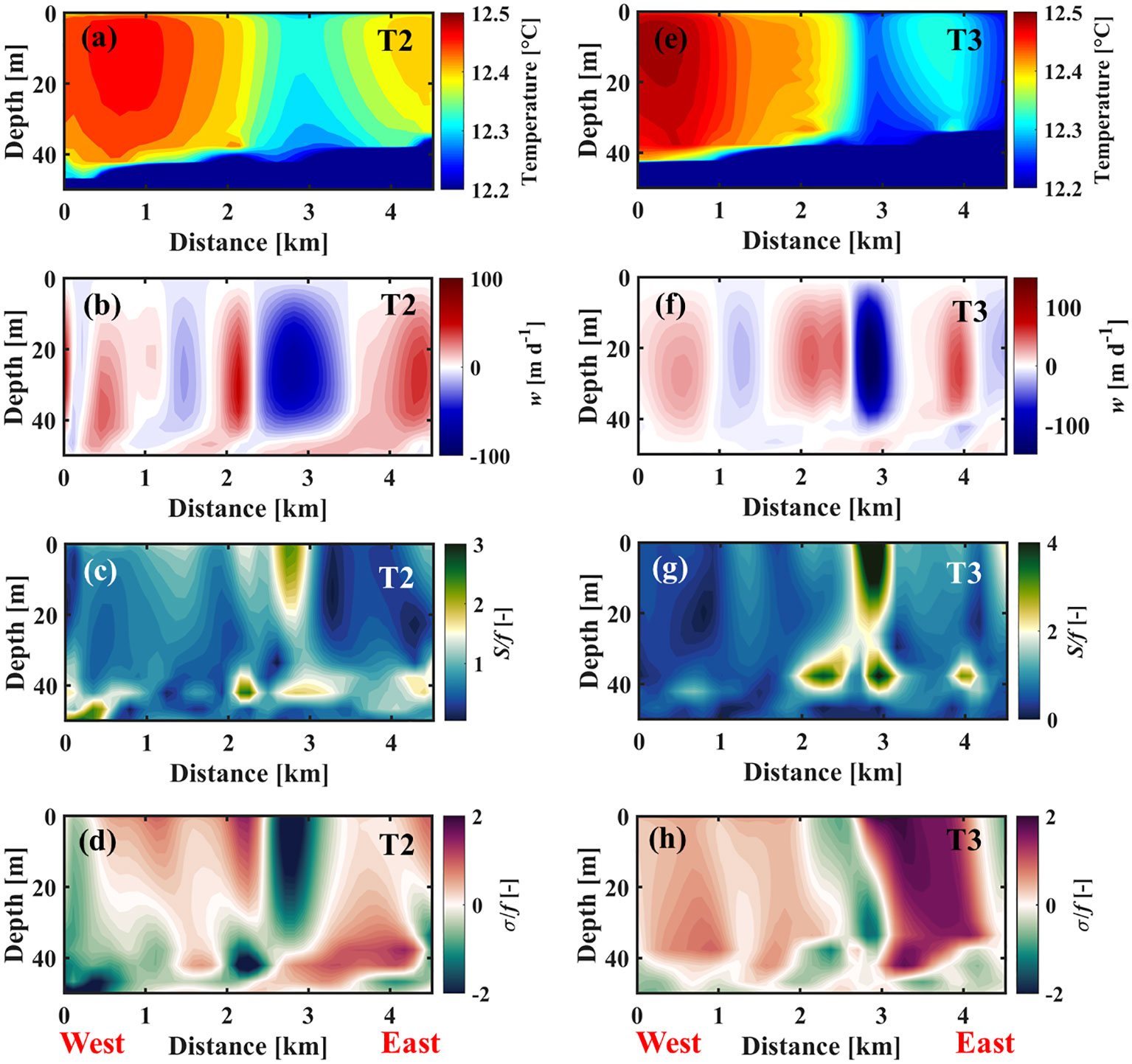
Figure 6 Numerical results for 25 November 2020 along transects T2 and T3 shown in Figure 5A. Simulated profiles of: (A) temperature, (B) vertical velocity, (C) normalized horizontal strain rate and (D) normalized divergence parameters along transect T2. Simulated profiles of: (E) temperature, (F) vertical velocity, (G) normalized horizontal strain rate, and (H) normalized divergence parameters along transect T3. Compare the modeled temperature patterns to the measured ones shown in Figure 5.

The measured temperature in different depth layers and the computed stratification strength ($N^2$) along transects T2 and T3 are given in Figure 7. Similar to the October observations, there is an increase in stratification strength in the SML on both sides of the cold filament and of the frontal regions (Figures 7A, C). The increase in N² reaches up to 2 × 10^-5 s^-2 in the deep mixed layer next to the cold filament (Figures 7E, F). The numerical model accurately captured the formation of submesoscale filaments induced by the background strain field (Figure 7). However, it was not able to resolve the increase in stratification strength around cold filaments and fronts (Figures 7B, D). The primary cause of this limitation can be attributed to the use of the K-Profile-Parameterization (KPP) turbulent model in the present study, which mainly addresses vertical momentum and temperature fluxes by only focusing on vertical gradients of properties (Large et al., 1994). However, submesoscale dynamics have revealed their potential to generate significant Vertical Buoyancy Flux (VBF), playing a pivotal role in shaping the stratification of the upper ocean (Zhang Z. et al., 2023). Considering that current ocean and lake models do not possess the capability to directly represent these important submesoscale dynamics, several studies have proposed new parameterizations for estimating VBF induced by submesoscale dynamics to improve the performance of current ocean models (e.g., Fox-Kemper et al., 2008; Bachman et al., 2017; Zhang J. et al., 2023). High-resolution Large-Eddy Simulations (LES) can also be used to resolve these small-scale instabilities associated with submesoscale processes (Thomas et al., 2013; Thomas et al., 2016). Nonetheless, a high-resolution model such as the one used in the present study can realistically evaluate conditions for various types of submesoscale instability (e.g., Chrysagi et al., 2021). In the near-surface layers, the stratification strength is negative primarily as a result of the cooling that occurred during the field campaign. More details about the atmospheric conditions during the field campaign are given in the Discussion section.

FIGURE 7

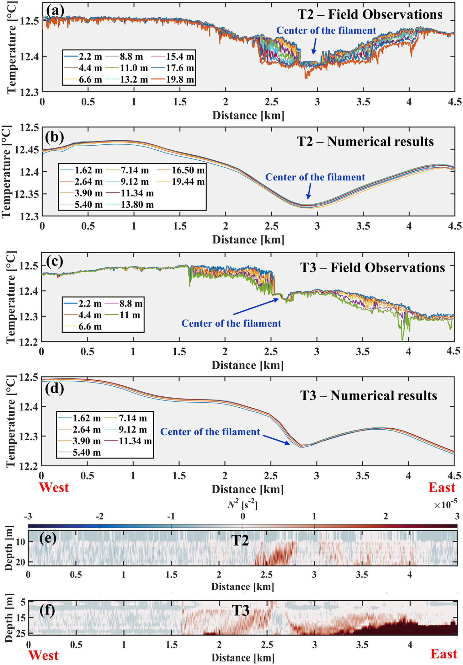
Figure 7 Field observations and numerical results for 25 November 2020 along transects T2 and T3 shown in Figure 5A. (A) Measured and (B) simulated temperatures along transect T2 for different depth layers in the SML. (C) Measured and (D) simulated temperature along transect T3 for different depth layers in the SML. Depth layers are given in the panels. (E, F) Estimated stratification strength, N², based on the measured temperature profiles along transects T2 and T3, respectively.

3.2 Passive tracer distribution caused by secondary circulation

The vertical distribution of physical and biological tracers in lakes can be influenced by intense vertical velocities associated with submesoscale secondary circulations. Acoustic backscatter is commonly used to measure the vertical distribution of a wide range of physical and biological parameters in the water column, including suspended sediments (Soulignac et al., 2021; Chalov et al., 2022) and zooplankton (Simonecelli et al., 2019). In addition to measuring vertical profiles of current velocity, Acoustic Doppler Current Profilers (ADCP) provide information on the particle distribution in the water column. The intensity of ADCP backscattering is affected by a number of factors, including the distance from the sensor, the amount of attenuation caused by the water and the concentration of suspended particles (Kim and Voulgaris, 2003; Chalov et al., 2022). Following Deines (1999), ADCP backscattering measurements are converted into volume-backscattering strength (measured in dB).

3.2.1 Backscattering Intensity (BI) along transect T1 on 19 October 2020

The estimated Backscattering Intensity (BI) along transect T1 on 19 October 2020 (Figure 3A) is shown in Figure 8A. In the epilimnion layer, BI ranges from 50 dB to 70 dB. Within the upper water column (down to 30-m depth), higher BI was measured at the cold filament locations. The areas with higher BI have almost the same width as the cold filaments. There are two areas with low BI adjacent to the cold filaments, where it was expected that upwelling would occur due to secondary circulation (Figure 4F). In addition, the effect of upwelling on BI induced by cyclonic circulation is evident in the near-surface layer of CC in the southern part of the lake (Figure 8A). Due to divergent flows in the near-surface layers and convergent flows in the deeper layers, water from deeper layers can be brought up into the mixed layer in the center of the CC (Hamze-Ziabari et al., 2023). The turbidity of upwelled water from greater depths is expected to be lower than that of near-surface waters. On the other hand, anticyclonic circulations cause a convergence of the flow in the near-surface layers, resulting in the downward movement of pollutants and particles. The BI patterns in the northern part of the lake display characteristics of large-scale downwelling caused by AC. In general, BI signals within the mixed layer are stronger in AC than in CC, suggesting a higher scatter concentration in AC.

FIGURE 8

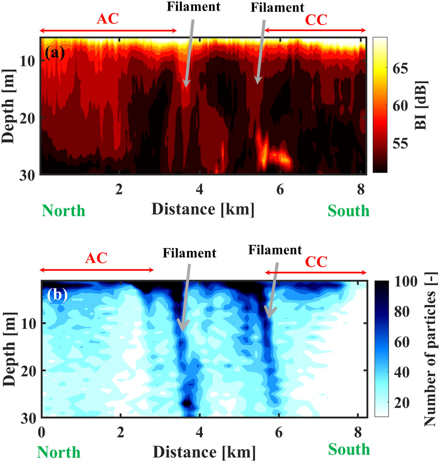
Figure 8 For 19 October 2020 along transect T1 in the western part of the Grand Lac shown in Figure 3A: (A) Filled contour plot of the observed Acoustic Doppler Current Profiler (ADCP) volume backscattering intensity (BI). (B) Filled contour plot of the number of particles obtained from the particle tracking results. The location of filaments, anticyclonic circulation (AC) and cyclonic circulation (CC) observed or simulated (see Figure 4) are marked with black and white arrows.

3.2.2 Particle tracking on 19 October 2020

Forward particle tracking was used to further investigate the effect of submesoscale and mesoscale currents on the horizontal and vertical distribution of passive tracers in Lake Geneva. The particles were uniformly released at every grid point in the deep (> 100 m) pelagic area of the Grand Lac (Figure 9A), where cyclonic and anticyclonic circulations were expected. A total of 345,097 particles were continuously released every hour in each depth layer (down to 44 m) during the 24 h prior to the field campaign on 19 October 2020. The fate of these 8,282,328 particles was monitored over the following 24 h. In the horizontal particle distribution, there was an accumulation of particles in the cold filaments that was coherent between all depth layers (Figures 9B‒E). This suggests that within the submesoscale filaments, particles are subducted to deeper layers. Filamentary accumulation of particles occurred at the edges of CC and AC (Figure 3A).

FIGURE 9

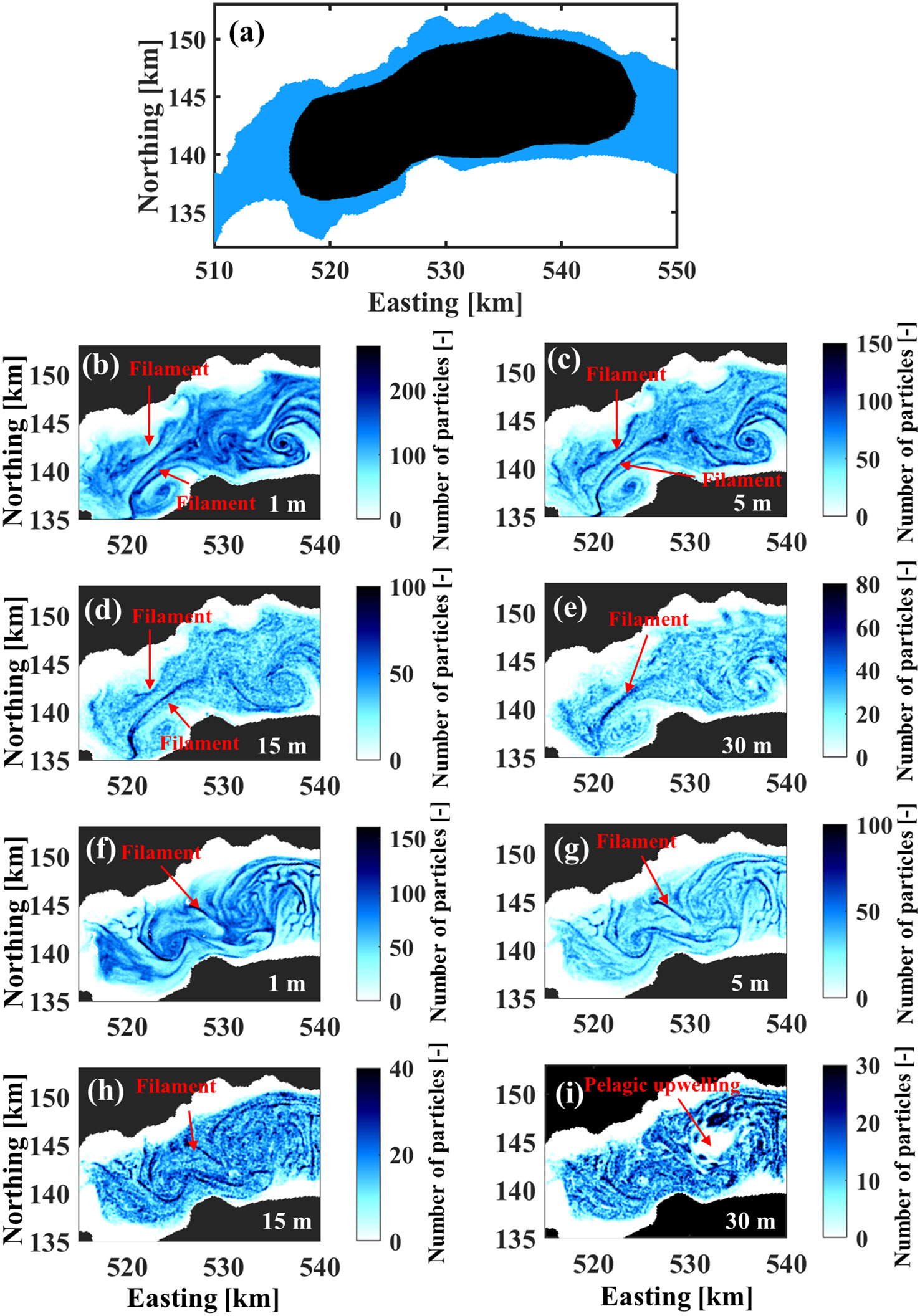
Figure 9 (A) Area (in black; > 100-m depth) where particles for forward tracking were uniformly released in the western and central parts of the Grand Lac basin in the near-surface layer (> 5 m depth). (B–E) Results of forward particle tracking for depths of 1, 5, 15 and 30 m at 12:00, 19 October 2020. (F–I) Results of forward particle tracking for depths 1, 5, 15 and 30 m at 12:00, 25 November 2020.

Figure 8B illustrates the vertical profiles of the particle distribution along transect T1 on 19 October 2020. At the filament locations, particles penetrated down to 30 m. BI exhibits a similar pattern in terms of the width and location where particles accumulated in the filament locations (Figure 8A). The patterns observed in BI signals are consistent with the distribution of passive tracers that is affected by mesoscale circulations. Particles in the AC center are transported to deeper layers by pelagic downwelling, whereas within CC, particles are transported from deeper layers to near-surface layers by pelagic upwelling. As a result, there are fewer particles in the deep epilimnion layers in the CC center, as opposed to the AC center where particles are transported downwards and accumulate in the deeper epilimnion layers.

3.2.3 Backscattering intensity on 25 November 2020

The BI patterns along transects T2 and T3 measured on 25 November 2020 are shown in Figures 10A, C, respectively. In both transects, there are strong backscattering signals near the cold filament. According to the particle tracking results, particles in the surface layers accumulate at the cold filament location and are then transported to deeper layers in both transects (Figures 10B, D). The backscattering signals are more intense in T3 than in T2. The number of particles that accumulate in transect T3 is also greater than in transect T2. The difference in intensity of backscattering signals and concentration of particles can be attributed to differences in the magnitude of the downwelling velocity at the cold filament location. As shown in Figures 6B, F, the downwelling velocity associated with secondary circulation is greater in transect T3 than in transect T2. Therefore, it can be expected that more particles accumulate and are transported to deeper layers in transect T3. Such strong vertical velocities associated with secondary circulations can potentially contribute to the rapid exchange of heat, mass, pollutants, carbon and oxygen between the lake surface and the thermocline layer. In transects T2 and T3, low backscattering signals were detected in the deeper epilimnion layers at the pelagic upwelling location in the CC.

FIGURE 10

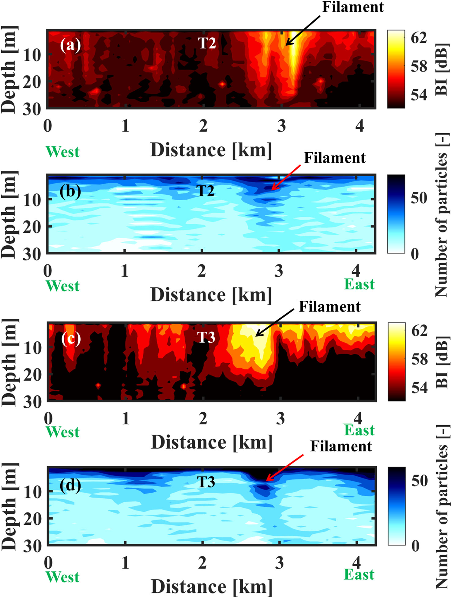
Figure 10 For 25 November 2020 along transects T2 and T3 in the central part of the Grand Lac shown in Figure 5A: (A) Filled contour plot of the observed ADCP backscattering intensity (BI) in transect T2. (B) Filled contour plot of the number of particles along T2 obtained from the results of particle tracking. (C) Filled contour plot of the observed ADCP backscattering intensity (BI) in transect T3. (D) Filled contour plot of the number of particles along T3 obtained from the results of particle tracking.

3.2.4 Particle tracking on 25 November 2020

For the 25 November 2020 particle tracking analysis, the horizontal distribution of particles obtained from forward particle tracking in different depth layers is given in Figures 9F–I. Unlike the filaments observed in October 2020, the filament on 25 November formed at the edge of the pelagic upwelling zone in the CC center and extended to the CC edge. The passive particles were completely depleted from the 30-m depth layer located in the thermocline and upwelled to the surface due to intense pelagic upwelling at the CC center (Figure 9I). Upwelled particles then accumulated at the CC edge in diverse filamentary patterns (Figure 9F). Thus, the source of cold water in the cold filament is the thermocline.

4 Discussion

4.1 Physical cause of surface mixed layer (SML) re-stratification

Wind stress and surface heating/cooling can either stabilize or destabilize the water column in frontal or filamentary regions (Mahadevan, 2016). The average wind speed and net upward Heat Flux (HF) obtained from COSMO data during the field campaigns in October and November 2020 are presented in Figure 11. HF includes latent flux, sensible flux, net longwave radiation and net shortwave radiation. If HF is positive, the lake surface is cooling and the resulting buoyancy loss suppresses the mechanism for re-stratification of the SML in the frontal zone (Chrysagi et al., 2021). Surface heating occurred at the study site during the October 2020 field campaign (Figure 11B). During the November field campaign, however, surface cooling was observed in the filamentary region (Figure 11D).

FIGURE 11

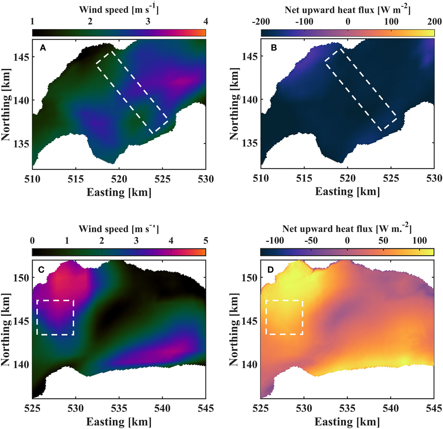
Figure 11 (A) Average wind speed and (B) net upward heat flux extracted from COSMO data during the field campaign on 19 October 2020 in the western part of the Grand Lac basin. (C) Average wind speed and (D) net upward heat flux extracted from COSMO data during the field campaign on 25 November 2020 in the central part of the Grand Lac basin. White dashed-lined rectangles and squares indicate the study areas. Colorbars give the parameter ranges.

Wind-induced Ekman transport may enhance or weaken the re-stratification of the SML in the frontal region (Thomas et al., 2013; Mahadevan, 2016). The wind-driven overturning cells can act either in conjunction with or in opposition to the re-stratification cells, potentially enhancing or weakening the SML re-stratification process. However, wind speeds were negligible during both field campaigns (< 4 m s^-1; Figures 11A, C). Therefore, in the present study, Ekman transport does not play a role in the re-stratification of the SML. In addition, COSMO data as well as SML temperatures along the measured transects demonstrate the effects of surface cooling during the November field campaign. Although surface cooling can destabilize the SML, positive stratification is still observed in the deeper layers of the epilimnion (10-20 m) surrounding the cold filaments, indicating that a mechanism different from atmospheric forcing is responsible for the re-stratification of the deep SML.

To further investigate the potential mechanism driving the SML re-stratification, the conditions for the occurrence of gravitational (i.e., $N^2<0$), centrifugal or inertial instability (i.e., $N^2>0, {\xi }_{abs} =f+\xi <0$) and symmetric instability ($f{q}_{bc}\langle 0, \left|f{q}_{bc}\right|\rangle f{q}_{ver}, f{q}_{ver}>0, b_z>0$) are examined (Thomas et al., 2013; Bachman et al., 2017; Zhurbas et al., 2022). The results of the instability analysis for depth layers 5, 10, 15 and 20 m (Figures 12A-D) for 19 October 2020 indicate that a combination of Symmetric Instability (SI) and centrifugal instability coexist in the region where the anticyclonic and cyclonic circulations interact (Figure 12). SI is the dominant instability in the center of the lake, whereas centrifugal instability is more pronounced in the regions where cyclonic/anticyclonic circulations interact with the boundaries and littoral zones of the lake. Generally, the water column is stable in terms of gravitational instability, as was observed in the field campaign and modeling driven by COSMO data.

FIGURE 12

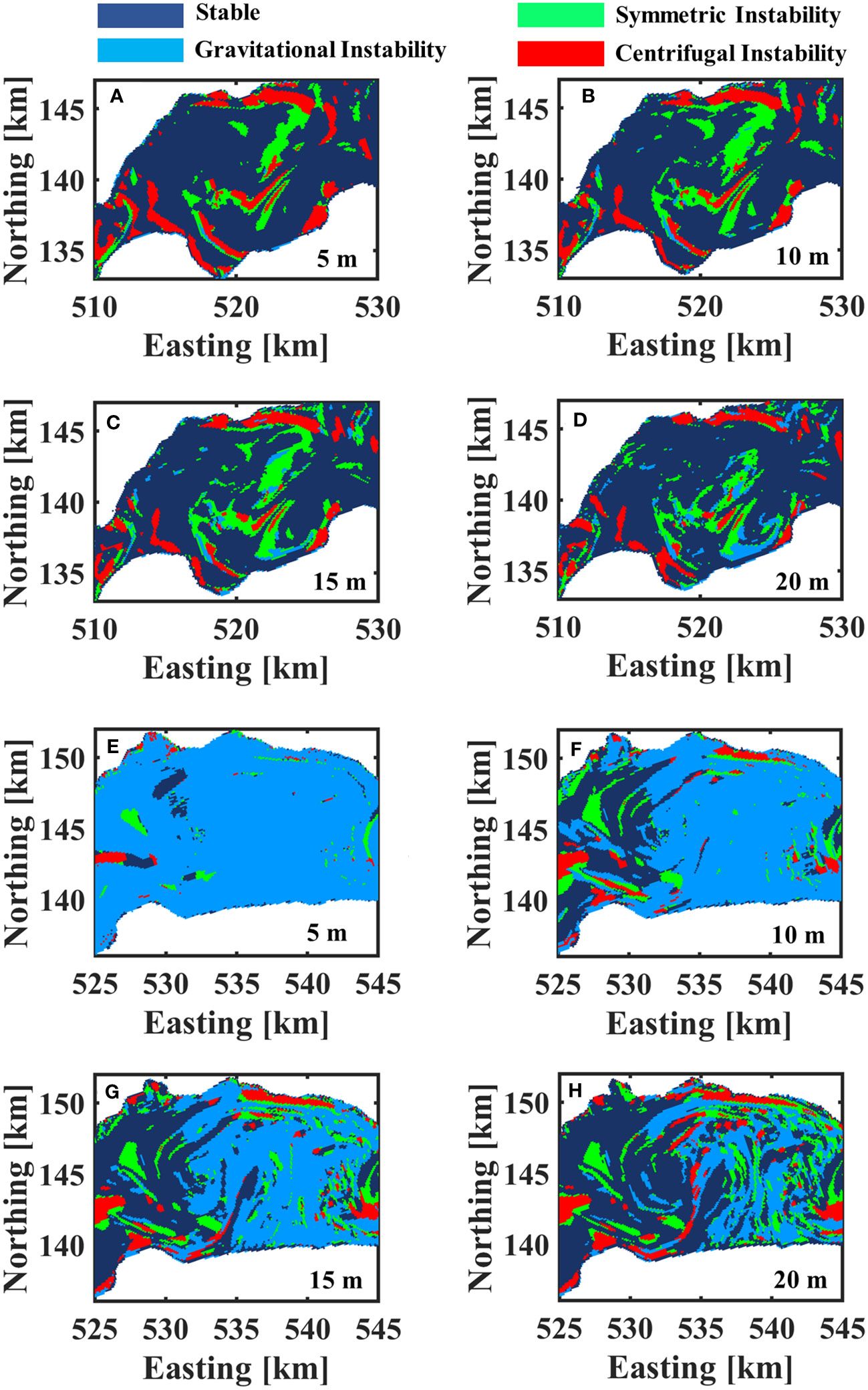
Figure 12 Classification of the study area based on the criteria of different kinds of submesoscale instability at different depth levels (5, 10, 15 and 20 m) for (A–D) 19 October 2020 in the western part of the Grand Lac basin and (E–H) 25 November 2020 in the central part of the Grand Lac basin. The color legend defines the type of instability.

It should be noted, however, that in November, the water column in most areas of the near-surface layers is unstably stratified and gravitational instability dominates due to convective surface cooling (Figures 12E, F). In addition, surface cooling can promote higher secondary SI (Thomas et al., 2013). According to the numerical results, SI is dominant in deeper layers (10 - 30 m) where the water column is more stable in terms of gravitational instability. Two areas next to the cold filaments are susceptible to SI. Therefore, the re-stratification of the water column in deeper layers on both sides of the cold filament can be attributed to the secondary circulation associated with SI, which can coexist with baroclinic instability (Verma et al., 2022). As a result, slantwise convection leads to vertical and horizontal exchange of water parcels; this can explain the increase of stratification strength in areas adjacent to the observed filaments (Gula et al., 2022) (Figures 4, 7). Furthermore, these submesoscale instabilities can be associated with the vertical exchange of nutrients and chlorophyll, primarily because of their role in the energy cascade and tracer variance from mesoscale to small-scale turbulence (Mahadevan, 2016; Lévy et al., 2018; Zhang J. et al., 2021; Chen et al., 2022).

4.2 Filaments: coherent pathways for subduction of passive tracers

The exchange of heat, mass and oxygen between the lake and the atmosphere can be greatly facilitated by high vertical velocities [O(100 m d^-1)] produced by submesoscale dynamics (Mahadevan, 2016; Lévy et al., 2018). In the pelagic zone of lakes, upwelling and downwelling associated with basin-scale or mesoscale circulations are considered to be the dominant physical mechanisms for the vertical transport of tracers (Hamze-Ziabari et al., 2023). However, it appears that vertical transport by submesoscale processes has previously been overlooked as an alternative. Secondary circulations associated with cold filaments are characterized by strong downward velocities within narrow regions, while strong upward velocities can develop over a wider area around the filament. Vertical velocities within filaments of O(100 m d^-1) were found (Figures 4, 6), which are significantly higher than those observed in geostrophic or quasi-geostrophic circulations, i.e., 10 m d^-1. The exchange of tracers between the SML and thermocline is, therefore, expected to be more significant in areas where secondary circulations occur.

To further investigate the effect of submesoscale filaments on the redistribution of passive tracers, forward particle tracking was applied to the computed 3D velocity field. The main objective was to illustrate the efficiency of transporting water parcels from the SML into the thermocline layer, a process called subduction (Freilich and Mahadevan, 2021), by the secondary circulation formed in frontal and filamentary zones. To achieve this, particles were released every hour at all possible grid points in the top 5 m of the water column in the deep, pelagic area (> 100-m depth) of the Grand Lac over a 24 h period (Figure 9A). Then, the fate of the released particles was monitored for the next 24 h. Two cases related to the weakly stratified conditions on 19 October and 25 November 2020 were investigated where the existence of submesoscale filaments was already revealed by field measurements in the pelagic area of the lake as discussed above (Figures 3–7).

On 19 October 2020, the average depth of the mixed layer base in the study area was ~15 m according to the numerical results. The particles were grouped into four classes based on their depths: C1 (depth ≤ 5 m; near-surface layer), C2 (5 m< depth ≤ 15 m; deep mixed layer), C3 (15 m< depth ≤ 25 m; thermocline layer) and C4 (depth > 25 m; hypolimnion layer). The temporal evolution of the particle distribution at 15-m depth, i.e., at the base of the deep mixed layer, is given in Figures 13A, C, E, G. Particles released in the near-surface layer are not evenly distributed in the pelagic zone with time. They were subducted into the base of the mixed layer inside the filamentary regions where the particle concentration gradually increased within a few hours after particle release ceased. Figure 13B shows that almost 30% of the particles were subducted into deeper layers, primarily into the deep mixed layer (C2), 24 h after particle release started. Nearly 50% of the released particles were subducted into the deeper layers (Figure 13H) and 21% of the released particles were subducted into the thermocline layer (C3) and the hypolimnion layer (C4) already 24 h after the particle release had ceased. After 48 h, 26% of particles were located in C2, indicating that within the thermocline and surface layers, particles are continuously being transported downward along coherent pathways.

FIGURE 13

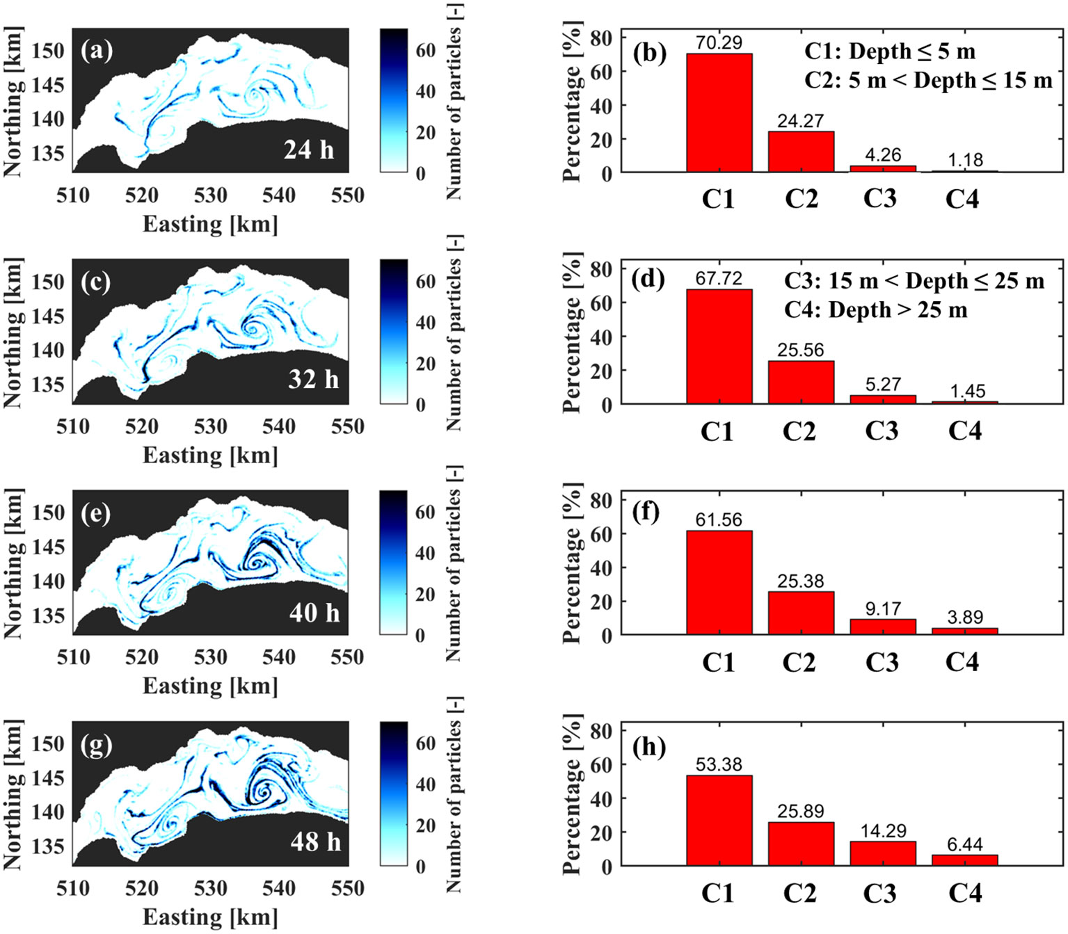
Figure 13 Results of forward particle tracking for 19 October 2020 in the Grand Lac basin. Particles were released in the near-surface layer (< 5-m depth; see Figure 9A). Left column: (A, C, E, G). Time development of particle concentration at the base of the mixed layer (~15 m). The time after the release of the particles is indicated in each panel. The legend gives the particle number range. Right column: (B, D, F, H). The corresponding percentage of particles in different depth classes (C1-C4). The depth range of the depth classes is identified in the panels. Note the decrease in the upper layer classes (C1 and C2) and the increase in the lower layer classes (C3 and C4) with time, indicating downward transport.

For the 25 November 2020 field observations, the particle tracking strategy described above illustrates the temporal evolution of particle concentrations at 25-m depth (Figure 14), which is the average depth of the SML base within the study area. Based on the depth of the SML and the thermocline layer, four different classes were defined (Figure 14). Note that only particles with $N^2>0$ are considered in Figure 14. Particles accumulated in the filamentary pathways within the cyclonic and anticyclonic circulations, especially at their edges (Figure 14). After 24 h, almost 40% of particles were transported to the deeper layer (C2 to C4; Figure 14B), mainly in the deep mixed layer (C2). Over time, more particles were subducted into the thermocline and hypolimnion layers (C3 and C4). After 48 h, ~ 70% of particles released in the near-surface layers were transported to deeper layers (Figure 14H). Almost 23% of particles had passed through the thermocline layer and reached the hypolimnion layer. In contrast to the October analysis, the subducted particles from the SML did not accumulate in the thermocline and were able to reach deeper layers. It is known that the thermocline can act as a physical barrier for the transport of momentum and tracers in lakes (Hamze-Ziabari et al., 2022c). However, the thermocline is not an absolute barrier and gradually weakens due to seasonal cooling, which starts in early fall. In Lake Geneva, the thermocline is generally much stronger in October than in November (Hamze-Ziabari et al., 2022c). Thus, the increased subduction of particles in November can be attributed to the reduced strength of the thermocline, which no longer confines vertical motions associated with mesoscale and submesoscale flows.

FIGURE 14

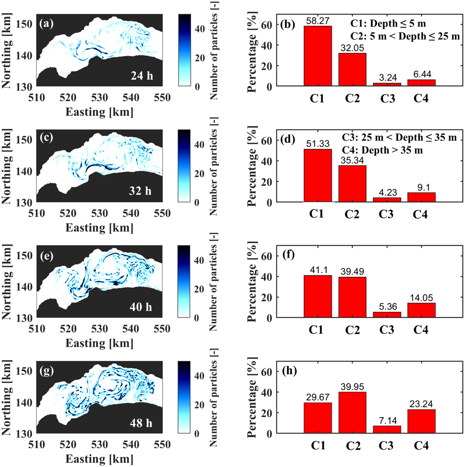
Figure 14 Results of forward particle tracking for 25 November 2020 in the Grand Lac basin. Particles were released in the near-surface layer (< 5-m depth; see Figure 9A). Left column: (A, C, E, G). Time development of particle concentration at the base of the mixed layer (~25 m). The time after the release of the particles is shown in each panel. The legend gives the particle number range. Right column: (B, D, F, H). The corresponding percentage of particles in different depth classes (C1-C4). The depth range of the depth classes is identified in the panels. Note that the classes are different than those in Figure 13 and the decrease in the upper layer classes (C1 and C2) and the increase in the lower layer classes (C3 and C4) with time, indicating downward transport, in particular, below the thermocline (C4).

Several studies in oceans have shown that submesoscale processes are mostly active in winter and spring and that the vertical motions associated with such processes increase during this period (Callies et al., 2015; Zhang J. et al., 2021; Ding et al., 2022; Taylor and Thompson, 2023). During summer and fall, however, the shallower mixed layer and stronger thermocline layer confine the vertical motion of submesoscale flows (Li et al., 2022). Larger variances in vertical velocities, divergence and vorticity are reported in wintertime (Berta et al., 2020). The submesoscale processes can be energized by baroclinic instabilities in the deep mixed layer during wintertime (Taylor and Thompson, 2023). The submesoscale vertical motion can potentially carry heat and atmospheric gases into deeper layers below the thermocline and even to the benthic layers (Callies et al., 2015), thereby potentially playing a role in deep-water winter mixing. The effects of submesoscale processes on winter mixing have generally been overlooked in lake studies, mainly due to limited field observations and low-resolution numerical models. The high-resolution numerical model and particle tracking results presented here indicate that submesoscale dynamics can contribute significantly to the exchange of tracers between the near-surface layer and the hypolimnion of Lake Geneva on a timescale of a few hours. Further research is needed in order to quantify the contribution of submesoscale flows to the exchange of water parcels between the near-surface layer and the hypolimnion layer of large lakes, especially in wintertime.

4.3 Filaments: Implications for dissolved oxygen variability

Few field studies have investigated the biochemical variability caused by submesoscale filaments in oceans (Lévy et al., 2018; Kaiser et al., 2021); however, no observations are available for lakes. Due to the ephemeral nature of submesoscale processes, it is difficult to establish a clear connection between secondary circulation and spatial variability of ecological parameters, such as Dissolved Oxygen (DO) in lakes or oceans. Phytoplankton growth in lakes mainly depends on light, nutrient availability, water temperature and the stability of the water column (MacIntyre et al., 2006; Bouffard et al., 2018). The present results indicate that submesoscale processes associated with cold filaments may have a significant impact on all these factors. The downward fluxes at the center of cold filaments can result in the export of nutrients and organic matter below the euphotic zone, which can reduce primary production. On the other hand, upwelling cells associated with secondary circulation can transport nutrient-rich water from the thermocline and deeper layers into the euphotic zone, thereby increasing phytoplankton abundance (Lévy et al., 2018).

Two field campaigns on 16 and 19 October 2021 examined the spatial DO variability adjacent to two cold filaments that formed in the center of CC (Figure 15A) and in the peripheries of CC and AC (Figure 15B). On 16 October 2021, transect T4, consisting of 15 measurement points at 300-m intervals, was measured inside the CC located in the central part of the Grand Lac. At the periphery of pelagic upwelling in the center of CC, a cold filament was present as predicted by the numerical results. The measured temperature profiles indicated significant pelagic upwelling along transect T4 at the center of CC (Figure 15C) and a narrow cold filament was detected ~1.5 km from the center. The DO profiles show that at the location of the cold filament, the DO levels in the SML are lower compared to the adjacent waters (Figure 15E). The spatial variability of DO in the SML can reach 0.2-0.5 mg l^-1 in the filament location. Interestingly, on each side of the cold filament, a distinct cell with higher levels of DO formed.

FIGURE 15

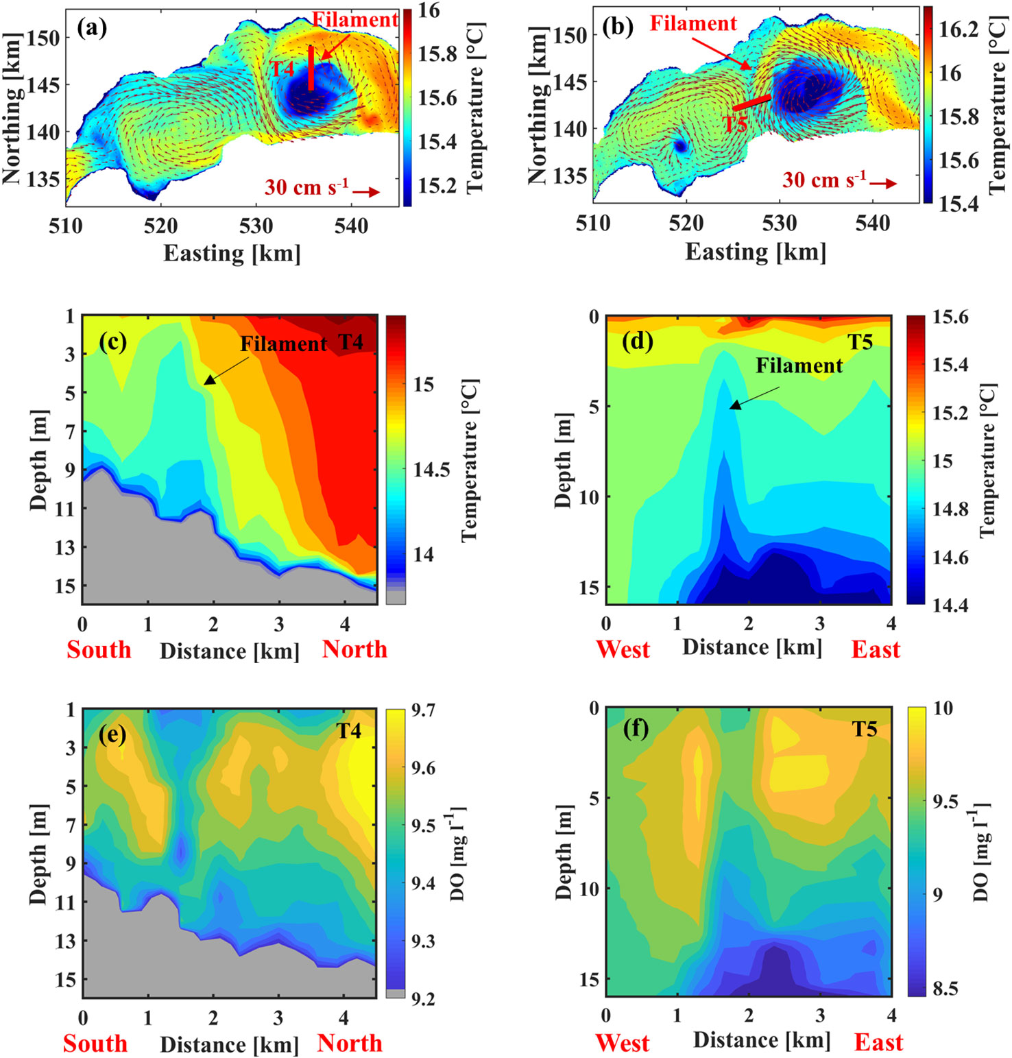
Figure 15 Numerical results of the temperature (colors; see colorbar) and velocity (red arrows; see reference arrow) fields at 1-m depth in the Grand Lac basin for (A) 16 October 2021 and (B) 19 October 2021, showing a strong CC in the center and a weaker AC in the western part. The red lines mark transects T4 and T5 where field measurements were taken. Measured profiles of temperature in the mixed layer on (C) 16 October and (D) 19 October. Measured profiles of Dissolved Oxygen (DO) in the mixed layer on (E) 16 October and (F) 19 October 2021. Note that on both sides of the cold filament, a distinct cell with higher levels of DO formed, while the level of DO within the cold filaments was lower with respect to the ambient waters.

At the edge of mesoscale circulations, large density gradients and horizontal strains induced by strong eddy/gyre currents can lead to the formation of submesoscale filaments/fronts. Intense secondary circulation is expected at the edge of mesoscale circulations, which can impact the supply of nutrients and chlorophyll. On 19 October 2021, the numerical model predicted the formation of a dipole consisting of a cyclonic (CC) in the central part of the Grand Lac basin and an anticyclonic (AC) circulation in the western part (Figure 15B). Transect T5 was based on numerical results that predicted that a cold filament formed in the area where the cyclonic and anticyclonic circulations interacted with each other. Temperature and DO profiles along transect T5 confirm this. A cold narrow region can be detected at a distance of ~1.5 km from the west. In the SML, the corresponding DO levels at the location of the cold filament are lower compared to the adjacent waters (Figure 15F). The spatial variability of DO in the SML reaches 0.1 - 0.5 mg l^-1 in the filament location. Similar to 16 October, an increase in DO levels appears on both sides of the filament as two distinct cells.

The photic layer in oligo-to mesotrophic lakes, such as Lake Geneva, is often nutrient limited during late summer and autumn, primarily due to accelerated physiological processes that include nutrient uptake, growth, respiration, and the onset of thermal stratification during spring (Berger et al., 2010; Watanabe et al., 2016; Bouffard et al., 2018). This nutrient depletion extends down to depths of 35-50 meters in Lake Geneva during summer and autumn (Bouffard et al., 2018). If upwelling cells associated with secondary circulation bring nutrients into in the photic layer, this can lead to an increase in primary production and thus increased DO levels (Lévy et al., 2012). However, as depicted in Figures 15C and D, the mixed layer depths within the observed filaments are ~ 15 meters. This indicates that the increase of DO in the vicinity of these observed filaments cannot be attributed to the upward nutrient flux resulting from upwelling induced by secondary circulation, since its effects are confined to a depth of 15 m (i.e., the mixed layer depth).

Figures 15A, B suggest that the observed cold water filaments originate either from upwelling at the center of a cyclonic gyre or from nearshore upwelling. Previous studies on Lake Geneva have shown that nutrient-rich water can reach the mixed layer through pelagic (Hamze-Ziabari et al., 2023; Figure 9I) or nearshore upwelling (Reiss et al., 2020) from the deep thermocline and hypolimnion. It can therefore be expected that the biological processes within filaments are enhanced due to nutrient-rich upwelled water. However, Figures 15E, F reveal that the DO levels inside the filaments are lower than in the adjacent water. In addition, the strong downward velocity within the filament, attributed to secondary circulation, would enhance the exchange of oxygen between the atmosphere and the mixed layer, which contradicts the observations in October. However, the reduction in DO within the cold filament can also be explained by strong downwelling at the center of the filament, inhibiting the export of nutrients by mesoscale upwelling from deeper layers into the photic layer. This, in turn, reduces primary production and the associated DO production. While our field campaigns were concentrated in the upwelling zones, resulting in increased DO levels due to biological processes in the surface mixed layer (SML) in most areas, the strong downwelling at the center of the cold filament could account for the reduced DO levels within the filament.

Our field observations indicate that under weak stratification conditions, the SML can undergo re-stratification adjacent to the cold filaments. This shear-driven vertical stratification prolongs the residence time of phytoplankton in the euphotic zone, potentially leading to localized blooms in the re-stratified areas compared to the surrounding turbulent mixed waters (Lévy et al., 2018). The patches of higher DO levels in the vicinity of the filaments in the SML may also be attributed to this process. In general, these DO observations suggest that secondary circulations induced by submesoscale filaments can influence biological activity, given that their time scales are similar to those of phytoplankton growth (Mahadevan, 2016). Although these localized blooms may not significantly impact the overall seasonal productivity of lakes or oceans, they are likely to affect the distribution and succession of seasonal species and the structure of local communities (Lévy et al., 2012; Lévy et al., 2018), contributing to patchiness.

5 Summary and conclusions

The role submesoscale filaments play in re-stratifying the Surface Mixed Layer (SML) was investigated for the first time in a lake by combining comprehensive field observations, high-resolution 3D numerical simulations and particle-tracking in large Lake Geneva. Particle-tracking allowed determining how fluid parcels are transported horizontally and vertically in the presence of submesoscale filaments. These unique field measurements were used to quantify the stratification strength variability, vertical velocities and Dissolved Oxygen (DO) concentrations in proximity to submesoscale filaments. Based on realistic numerical modeling and field observations, the following conclusions can be drawn from the presented analysis:

● Submesoscale cold filaments can form at the edges of both cyclonic and anticyclonic circulations (gyres and eddies) under weakly stratified conditions.

● Submesoscale cold filaments can also form in the pelagic upwelling zone at the center of a cyclonic circulation.

● Under weakly stratified conditions, the stratification strength, N², can increase in areas adjacent to the cold filaments. The enhancement of stratification strength reached O(10^-5 s^-2) under atmospheric heating and cooling conditions in October and November 2020, respectively.

● Numerical results indicate that a combination of Symmetric Instability (SI) and centrifugal instability can potentially occur in proximity to the center of cold filaments. Slantwise convection associated with SI, a previously overlooked process in lakes, can explain enhanced stratification strength in areas adjacent to the observed filaments.

● Patterns of secondary circulation can be detected in Acoustic Doppler Current Profiler (ADCP) backscattering signals, as confirmed by numerical results and forward particle tracking.

● Particle tracking results indicated that passive tracers accumulate in the center of the cold filament and are transported to deeper layers. More than 20% of the particles were subducted into the thermocline and the hypolimnion layers due to secondary circulation associated with submesoscale filaments/fronts.

● Dissolved oxygen variability in the observed cold filaments reached 0.1-0.5 mg l^-1 under weakly stratified conditions.

● On each side of cold filaments, distinct cells with higher levels of dissolved oxygen formed, while the DO level within the cold filaments was lower than that in the ambient waters.

Multiscale rotational flow fields (e.g., gyres and eddies) and pelagic/coastal upwelling are ubiquitous in Lake Geneva and other large lakes, as well as in oceans, which suggests that the frontogenesis and filamentogenesis discussed here occur regularly in these water bodies. Consequently, they can affect the interplay of complex 3D bio-chemo-physical processes in both large lakes and oceans. Submesoscale filaments/fronts cause vertical re-stratification of the SML and decrease vertical mixing, thereby potentially affecting phytoplankton residence times in the euphotic zone. Secondary circulation associated with filaments or fronts, for example, can impact on the phytoplankton growth cycle due to their effects on the vertical distribution of nutrients and pollutants. Furthermore, submesoscale filaments and the associated secondary circulations can accumulate surface materials and create vertical pathways enabling rapid transport to deeper layers, in particular, when stratification strength is weak.

The present study investigated submesoscale filament dynamics in the SML in a large lake. However, these unique results are also valid in oceans where field verification is much more difficult. Further research is needed to improve the understanding of spatial and seasonal variability caused by submesoscale and mesoscale processes in large lake and ocean ecosystems.

Data availability statement

The raw data supporting the conclusions of this article will be made available by the authors, without undue reservation.

Author contributions

SH-Z and MF conducted the field campaigns. SH-Z and R.S.R. implemented the numerical simulation. SH-Z conducted the data analyses, created the figures, and led the writing of the manuscript. UL and DB led the revision and critically reviewed the manuscript. All authors provided feedback on the manuscript. All authors contributed to the article and approved the submitted version.

Funding

This research was supported by the Swiss National Science Foundation (SNSF Grant 178866).

Acknowledgments

The spatiotemporal meteorological data were provided by the Federal Office of Meteorology and Climatology in Switzerland (MeteoSwiss). We also extend our appreciation to the Commission Internationale pour la Protection des Eaux du Léman (CIPEL) for in situ temperature measurements. Water temperature profiles were collected at the CIPEL SHL2 station for 2019-2020 by the Eco-Informatics ORE INRA Team at the French National Institute for Agricultural Research (SOERE OLA-IS, INRA Thonon-les-Bains, France).

Conflict of interest

The authors declare that the research was conducted in the absence of any commercial or financial relationships that could be construed as a potential conflict of interest.

Publisher’s note

All claims expressed in this article are solely those of the authors and do not necessarily represent those of their affiliated organizations, or those of the publisher, the editors and the reviewers. Any product that may be evaluated in this article, or claim that may be made by its manufacturer, is not guaranteed or endorsed by the publisher.

References

Adams K. A., Hosegood P., Taylor J. R., Sallée J. B., Bachman S., Torres R., et al. (2017). Frontal circulation and submesoscale variability during the formation of a Southern Ocean mesoscale eddy. J. Phys. Oceanography 47 (7), 1737–1753. doi: 10.1175/JPO-D-16-0266.1

CrossRef Full Text | Google Scholar

Aravind H. M., Verma V., Sarkar S., Freilich M. A., Mahadevan A., Haley P. J., et al. (2023). Lagrangian surface signatures reveal upper-ocean vertical displacement conduits near oceanic density fronts. Ocean Model. 181, 102136. doi: 10.1016/j.ocemod.2022.102136

CrossRef Full Text | Google Scholar

Archer M., Schaeffer A., Keating S., Roughan M., Holmes R., Siegelman L. (2020). Observations of submesoscale variability and frontal subduction within the mesoscale eddy field of the Tasman Sea. J. Phys. Oceanography 50, 1509–1529. doi: 10.1175/JPO-D-19-0131.1

CrossRef Full Text | Google Scholar

Bachman S. D., Fox-Kemper B., Taylor J. R., Thomas L. N. (2017). Parameterization of frontal symmetric instabilities. I: Theory for resolved fronts. Ocean Model. 109, 72–95. doi: 10.1016/j.ocemod.2016.12.003

CrossRef Full Text | Google Scholar

Bauer S. W., Graf W. H., Mortimer C. H., Perrinjaquet C. (1981). Inertial motion in Lake Geneva (Le léman). Arch. Meteorology Geophysics Bioclimatology Ser. A 30, 289–312. doi: 10.1007/BF02257850

CrossRef Full Text | Google Scholar

Berger S. A., Diehl S., Stibor H., Trommer G., Ruhenstroth M. (2010). Water temperature and stratification depth independently shift cardinal events during plankton spring succession. Global Change Biol. 16 (7), 1954–1965. doi: 10.1111/j.1365-2486.2009.02134.x

CrossRef Full Text | Google Scholar

Berta M., Griffa A., Haza A. C., Horstmann J., Huntley H. S., Ibrahim R., et al. (2020). Submesoscale kinematic properties in summer and winter surface flows in the northern Gulf of Mexico. J. Geophysical Research: Oceans 125, e2020JC016085. doi: 10.1029/2020JC016085

CrossRef Full Text | Google Scholar

Birch D. A., Young W. R., Franks P. J. S. (2008). Thin layers of plankton: Formation by shear and death by diffusion. Deep Sea Res. Part I: Oceanographic Res. Papers 55, 277–295. doi: 10.1016/j.dsr.2007.11.009

CrossRef Full Text | Google Scholar

Boccaletti G., Ferrari R., Fox-Kemper B. (2007). Mixed layer instabilities and restratification. J. Phys. Oceanography 37, 2228–2250. doi: 10.1175/JPO3101.1

CrossRef Full Text | Google Scholar

Bouffard D., Kiefer I., Wüest A., Wunderle S., Odermatt D. (2018). Are surface temperature and chlorophyll in a large deep lake related? An analysis based on satellite observations in synergy with hydrodynamic modelling and in-situ data. Remote Sens. Environ. 209, 510–523. doi: 10.1016/j.rse.2018.02.056

CrossRef Full Text | Google Scholar

Bouffard D., Lemmin U. (2013). Kelvin waves in Lake Geneva. J. Great Lakes Res. 39, 637–645. doi: 10.1016/j.jglr.2013.09.005

CrossRef Full Text | Google Scholar

Bracco A., Liu G., Sun D. (2019). Mesoscale-submesoscale interactions in the Gulf of Mexico: From oil dispersion to climate. Chaos Solitons Fractals 119, 63–72. doi: 10.1016/j.chaos.2018.12.012

CrossRef Full Text | Google Scholar

Brannigan L. (2016). Intense submesoscale upwelling in anticyclonic eddies. Geophysical Res. Lett. 43, 3360–3369. doi: 10.1002/2016GL067926

CrossRef Full Text | Google Scholar

Brüggemann N., Eden C. (2015). Routes to dissipation under different dynamical conditions. J. Phys. Oceanography 45, 2149–2168. doi: 10.1175/JPO-D-14-0205.1

CrossRef Full Text | Google Scholar

Callies J., Ferrari R., Klymak J. M., Gula J. (2015). Seasonality in submesoscale turbulence. Nat. Commun. 6, 6862. doi: 10.1038/ncomms7862

PubMed Abstract | CrossRef Full Text | Google Scholar

Campanero R., Burgoa N., Fernández-Castro B., Valiente S., Nieto-Cid M., Martínez-Pérez A. M., et al. (2022). High-resolution variability of dissolved and suspended organic matter in the Cape Verde Frontal Zone. Front. Mar. Sci. 9. doi: 10.3389/fmars.2022.1006432

PubMed Abstract | CrossRef Full Text | Google Scholar

Capet X., McWilliams J. C., Molemaker M. J., Shchepetkin A. F. (2008). Mesoscale to submesoscale transition in the California current system. Part III: Energy balance and flux. J. Phys. Oceanography 38, 2256–2269. doi: 10.1175/2008JPO3810.1

CrossRef Full Text | Google Scholar

Carpenter J. R., Rodrigues A., Schultze L. K., Merckelbach L. M., Suzuki N., Baschek B., et al. (2020). Shear instability and turbulence within a submesoscale front following a storm. Geophysical Res. Lett. 47 (23), e2020GL090365. doi: 10.1029/2020GL090365

CrossRef Full Text | Google Scholar

Chalov S., Moreido V., Ivanov V., Chalova A. (2022). Assessing suspended sediment fluxes with acoustic Doppler current profilers: Case study from large rivers in Russia. Big Earth Data 6, 504–526. doi: 10.1080/20964471.2022.2116834

CrossRef Full Text | Google Scholar

Chen Y., Li Q. P., Yu J. (2022). Submesoscale variability of subsurface chlorophyll-a across eddy-driven fronts by glider observations. Prog. Oceanography 209, 102905. doi: 10.1016/j.pocean.2022.102905

CrossRef Full Text | Google Scholar

Choi J., Bracco A., Barkan R., Shchepetkin A. F., McWilliams J. C., Molemaker J. M. (2017). Submesoscale dynamics in the northern Gulf of Mexico. Part III: Lagrangian implications. J. Phys. Oceanography 47, 2361–2376. doi: 10.1175/JPO-D-17-0036.1

CrossRef Full Text | Google Scholar

Chrysagi E., Umlauf L., Holtermann P., Klingbeil K., Burchard H. (2021). High-resolution simulations of submesoscale processes in the Baltic Sea: The role of storm events. J. Geophysical Research: Oceans 126, e2020JC016411. doi: 10.1029/2020JC016411

CrossRef Full Text | Google Scholar

Cimatoribus A. A., Lemmin U., Barry D. A. (2019). Tracking Lagrangian transport in Lake Geneva: A 3D numerical modeling investigation. Limnology Oceanography 64, 1252–1269. doi: 10.1002/lno.11111

CrossRef Full Text | Google Scholar

Cimatoribus A. A., Lemmin U., Bouffard D., Barry D. A. (2018). Nonlinear dynamics of the nearshore boundary layer of a large lake (Lake Geneva). J. Geophysical Research: Oceans 123, 1016–1031. doi: 10.1002/2017JC013531

CrossRef Full Text | Google Scholar

Couvelard X., Dumas F., Garnier V., Ponte A. L., Talandier C., Treguier A. M. (2015). Mixed layer formation and restratification in presence of mesoscale and submesoscale turbulence. Ocean Model. 96, 243–253. doi: 10.1016/j.ocemod.2015.10.004

CrossRef Full Text | Google Scholar

D’Asaro E. A. (1988). Generation of submesoscale vortices: A new mechanism. J. Geophysical Research: Oceans 93 (C6), 6685–6693. doi: 10.1029/JC093iC06p06685

CrossRef Full Text | Google Scholar

D’Asaro E., Lee C., Rainville L., Harcourt R., Thomas L. (2011). Enhanced turbulence and energy dissipation at ocean fronts. Science 332 (6027), 318–322. doi: 10.1126/science.1201515

PubMed Abstract | CrossRef Full Text | Google Scholar

Deines K. L. (1999). “Backscatter estimation using broadband acoustic Doppler current profilers,” in Proceedings of the IEEE Sixth Working Conference on Current Measurement (Cat. No.99CH36331). (San Diego USA: IEEE) 249–253. doi: 10.1109/CCM.1999.755249

CrossRef Full Text | Google Scholar

Demarcq H., Reygondeau G., Alvain S., Vantrepotte V. (2012). Monitoring marine phytoplankton seasonality from space. Remote Sens. Environ. 117, 211–222. doi: 10.1016/j.rse.2011.09.019

CrossRef Full Text | Google Scholar

Dever M., Freilich M., Farrar J. T., Hodges B., Lanagan T., Baron A. J., et al. (2020). EcoCTD for profiling oceanic physical–biological properties from an underway ship. J. Atmospheric Oceanic Technol. 37 (5), 825–840. doi: 10.1175/JTECH-D-19-0145.1

CrossRef Full Text | Google Scholar

Ding Y., Xu L., Xie S.-P., Sasaki H., Zhang Z., Cao H., et al. (2022). Submesoscale frontal instabilities modulate large-scale distribution of the winter deep mixed layer in the Kuroshio-Oyashio extension. J. Geophysical Research: Oceans 127, e2022JC018915. doi: 10.1029/2022JC018915

CrossRef Full Text | Google Scholar

Djoumna G., Lamb K. G., Rao Y. R. (2014). Sensitivity of the parameterizations of vertical mixing and radiative heat fluxes on the seasonal evolution of the thermal structure of Lake Erie. Atmosphere-Ocean 52, 294–313. doi: 10.1080/07055900.2014.939824

CrossRef Full Text | Google Scholar

Döös K., Kjellsson J., Jönsson B. (2013). “TRACMASS—A lagrangian trajectory model,” in Preventive methods for coastal protection: towards the use of ocean dynamics for pollution control. Eds. Soomere T., Quak E. (Heidelberg: Springer International Publishing), 225–249. doi: 10.1007/978-3-319-00440-2_7

CrossRef Full Text | Google Scholar

Dorostkar A., Boegman L. (2013). Internal hydraulic jumps in a long narrow lake. Limnology Oceanography 58, 153–172. doi: 10.4319/lo.2013.58.1.0153

CrossRef Full Text | Google Scholar

Dorostkar A., Boegman L., Pollard A. (2017). Three-dimensional simulation of high-frequency nonlinear internal wave dynamics in Cayuga Lake. J. Geophysical Research: Oceans 122, 2183–2204. doi: 10.1002/2016JC011862

CrossRef Full Text | Google Scholar

Erickson Z. K., Thompson A. F. (2018). The seasonality of physically driven export at submesoscales in the northeast Atlantic Ocean. Global Biogeochemical Cycles 32, 1144–1162. doi: 10.1029/2018GB005927

CrossRef Full Text | Google Scholar

Fadeev E., Wietz M., von Appen W.-J., Iversen M. H., Nöthig E.-M., Engel A., et al. (2021). Submesoscale physicochemical dynamics directly shape bacterioplankton community structure in space and time. Limnology Oceanography 66, 2901–2913. doi: 10.1002/lno.11799

CrossRef Full Text | Google Scholar

Flierl G. R., Woods N. W. (2015). Copepod aggregations: Influences of physics and collective behavior. J. Stat. Phys. 158 (3), 665–698. doi: 10.1007/s10955-014-1162-0

CrossRef Full Text | Google Scholar

Forel F. A. (1892). Le léman: monographie limnologique (Lausanne, Switzerland: F. Rouge). doi: 10.5962/bhl.title.124608

CrossRef Full Text | Google Scholar

Foroughan M., Hamze-Ziabari S. M., Lemmin U., Barry D. A. (2022). A persistent submesoscale frontal slick: A novel marker of the mesoscale flow field in a large lake (Lake Geneva). Geophysical Res. Lett. 49, e2022GL100262. doi: 10.1029/2022GL100262

CrossRef Full Text | Google Scholar

Fox-Kemper B., Ferrari R., Hallberg R. (2008). Parameterization of mixed layer eddies. Part I: Theory and diagnosis. J. Phys. Oceanography 38 (6), 1145–1165. doi: 10.1175/2007JPO3792.1

CrossRef Full Text | Google Scholar

Freilich M., Mahadevan A. (2021). Coherent pathways for subduction from the surface mixed layer at ocean fronts. J. Geophysical Research: Oceans 126, e2020JC017042. doi: 10.1029/2020JC017042

CrossRef Full Text | Google Scholar

Grisouard N. (2018). Extraction of potential energy from geostrophic fronts by inertial-symmetric instabilities. J. Phys. Oceanography 48, 1033–1051. doi: 10.1175/JPO-D-17-0160.1

CrossRef Full Text | Google Scholar

Gula J., Molemaker M. J., McWilliams J. C. (2014). Submesoscale cold filaments in the Gulf Stream. J. Phys. Oceanography 44, 2617–2643. doi: 10.1175/JPO-D-14-0029.1

CrossRef Full Text | Google Scholar

Gula J., Taylor J., Shcherbina A., Mahadevan A. (2022). “Submesoscale processes and mixing,” in Ocean mixing. Eds. Meredith M., Naveira Garabato A. (Amsterdam: Elsevier), 181–214. doi: 10.1016/B978-0-12-821512-8.00015-3

CrossRef Full Text | Google Scholar

Hamze-Ziabari S. M., Foroughan M., Lemmin U., Barry D. A. (2022b). Monitoring mesoscale to submesoscale processes in large lakes with Sentinel-1 SAR imagery: The case of Lake Geneva. Remote Sens. 14, 4967. doi: 10.3390/rs14194967

CrossRef Full Text | Google Scholar

Hamze-Ziabari S. M., Lemmin U., Foroughan M., Reiss R. S., Barry D. A. (2023). Chimney-like intense pelagic upwelling in the center of basin-scale cyclonic gyres in large Lake Geneva. J. Geophysical Research: Oceans 128 (7), e2022JC019592. doi: 10.1029/2022JC019592

CrossRef Full Text | Google Scholar

Hamze-Ziabari S. M., Lemmin U., Soulignac F., Foroughan M., Barry D. A. (2022c). Basin-scale gyres and mesoscale eddies in large lakes: A novel procedure for their detection and characterization, assessed in Lake Geneva. Geoscientific Model. Dev. 15, 8785–8807. doi: 10.5194/gmd-15-8785-2022

CrossRef Full Text | Google Scholar

Hamze-Ziabari S. M., Razmi A. M., Lemmin U., Barry D. A. (2022a). Detecting submesoscale cold filaments in a basin-scale gyre in large, deep Lake Geneva (Switzerland/France). Geophysical Res. Lett. 49, e2021GL096185. doi: 10.1029/2021GL096185

CrossRef Full Text | Google Scholar

Hernández-Hernández N., Arístegui J., Montero M. F., Velasco-Senovilla E., Baltar F., Marrero-Díaz Á., et al. (2020). Drivers of plankton distribution across mesoscale eddies at submesoscale range. Front. Mar. Sci. 7. doi: 10.3389/fmars.2020.00667

CrossRef Full Text | Google Scholar

Hoskins B. J. (1974). The role of potential vorticity in symmetric stability and instability. Q. J. R. Meteorological Soc. 100, 480–482. doi: 10.1002/qj.49710042520

CrossRef Full Text | Google Scholar

Jiang Y., Dong J., Zhang X., Zhang W., Wang H., Zhang W. (2022). Evaluating the effects of a symmetric instability parameterization scheme in the Xisha-Zhongsha waters, South China Sea in winter. Front. Mar. Sci. 9, 985605. doi: 10.3389/fmars.2022.985605

CrossRef Full Text | Google Scholar

Kaiser P., Hagen W., von Appen W.-J., Niehoff B., Hildebrandt N., Auel H. (2021). Effects of a submesoscale oceanographic filament on zooplankton dynamics in the Arctic Marginal Ice Zone. Front. Mar. Sci. 8. doi: 10.3389/fmars.2021.625395

CrossRef Full Text | Google Scholar

Kim Y. H., Voulgaris G. (2003). Estimation of suspended sediment concentration in estuarine environments using acoustic backscatter from an ADCP (Corpus Christi, Texas, USA: Proceedings of the International Conference on Coastal Sediments 2003. CD-ROM Published by World Scientific Publishing Corp. and East Meets West Productions). Available at: https://www.seoe.sc.edu/gvoulgar/students/Kim/research/abstract_CS03.pdf, ISBN: ISBN 981-238-422.

Google Scholar

Klein P., Hua B. L., Lapeyre G., Capet X., Gentil S. L., Sasaki H. (2008). Upper ocean turbulence from high-resolution 3D simulations. J. Phys. Oceanography 38, 1748–1763. doi: 10.1175/2007JPO3773.1

CrossRef Full Text | Google Scholar

Klein P., Lapeyre G. (2009). The oceanic vertical pump induced by mesoscale and submesoscale turbulence. Annu. Rev. Mar. Sci. 1, 351–375. doi: 10.1146/annurev.marine.010908.163704

CrossRef Full Text | Google Scholar

Kock T., Baschek B., Wobbe F., Heineke M., Riethmueller R., Deschner S. C., et al. (2023). An advanced towed CTD chain for physical-biological high resolution in situ upper ocean measurements. Front. Mar. Sci. 10. doi: 10.3389/fmars.2023.1183061

CrossRef Full Text | Google Scholar

Large W. G., McWilliams J. C., Doney S. C. (1994). Oceanic vertical mixing: A review and a model with a nonlocal boundary layer parameterization. Rev. geophysics 32 (4), 363–403. doi: 10.1029/94RG01872

CrossRef Full Text | Google Scholar

Large W. G., Yeager S. G. (2004). Diurnal to decadal global forcing for ocean and sea-ice models: the data sets and flux climatologies, Tech. (Colorado, USA: NCAR/TN-460+ STR, National Center of Atmospheric Research, Boulder). doi: 10.5065/D6KK98Q6

CrossRef Full Text | Google Scholar

Lehahn Y., d’Ovidio F., Koren I. (2018). A satellite-based Lagrangian view on phytoplankton dynamics. Annu. Rev. Mar. Sci. 10, 99–119. doi: 10.1146/annurev-marine-121916-063204

CrossRef Full Text | Google Scholar

Lehahn Y., d’Ovidio F., Lévy M., Heifetz E. (2007). Stirring of the northeast Atlantic spring bloom: A Lagrangian analysis based on multisatellite data. J. Geophysical Research: Oceans 112. doi: 10.1029/2006JC003927

CrossRef Full Text | Google Scholar

Lemmin U. (2020). Insights into the dynamics of the deep hypolimnion of Lake Geneva as revealed by long-term temperature, oxygen, and current measurements. Limnology Oceanography 65, 2092–2107. doi: 10.1002/lno.11441

CrossRef Full Text | Google Scholar

Lemmin U., D’Adamo N. (1996). Summertime winds and direct cyclonic circulation: Observations from Lake Geneva. Annales Geophysicae 14, 1207–1220. doi: 10.1007/s00585-996-1207-z

CrossRef Full Text | Google Scholar

Lemmin U., Mortimer C. H., Bäuerle E. (2005). Internal seiche dynamics in Lake Geneva. Limnology Oceanography 50, 207–216. doi: 10.4319/lo.2005.50.1.0207

CrossRef Full Text | Google Scholar

Lévy M., Franks P. J. S., Smith K. S. (2018). The role of submesoscale currents in structuring marine ecosystems. Nat. Commun. 9, 4758. doi: 10.1038/s41467-018-07059-3

CrossRef Full Text | Google Scholar

Lévy M., Iovino D., Resplandy L., Klein P., Madec G., Tréguier A. M., et al. (2012). Large-scale impacts of submesoscale dynamics on phytoplankton: Local and remote effects. Ocean Model. 43–44, 77–93. doi: 10.1016/j.ocemod.2011.12.003

CrossRef Full Text | Google Scholar

Lévy M., Klein P., Tréguier A.-M. (2001). Impact of sub-mesoscale physics on production and subduction of phytoplankton in an oligotrophic regime. J. Mar. Res. 59, 535–565. doi: 10.1357/002224001762842181

CrossRef Full Text | Google Scholar

Lévy M., Martin A. P. (2013). The influence of mesoscale and submesoscale heterogeneity on ocean biogeochemical reactions. Global Biogeochemical Cycles 27 (4), 1139–1150. doi: 10.1002/2012GB004518

CrossRef Full Text | Google Scholar

Li L., Cheng X., Jing Z., Cao H., Feng T. (2022). Submesoscale motions and their seasonality in the northern Bay of Bengal. Acta Oceanologica Sin. 41, 1–13. doi: 10.1007/s13131-021-1847-6

CrossRef Full Text | Google Scholar

MacIntyre S., Sickman J. O., Goldthwait S. A., Kling G. W. (2006). Physical pathways of nutrient supply in a small, ultraoligotrophic arctic lake during summer stratification. Limnology Oceanography 51, 1107–1124. doi: 10.4319/lo.2006.51.2.1107

CrossRef Full Text | Google Scholar

Mahadevan A. (2016). The impact of submesoscale physics on primary productivity of plankton. Annu. Rev. Mar. Sci. 8, 161–184. doi: 10.1146/annurev-marine-010814-015912

CrossRef Full Text | Google Scholar

Mangolte I., Lévy M., Dutkiewicz S., Clayton S., Jahn O. (2022). Plankton community response to fronts: winners and losers. J. Plankton Res. 44, 241–258. doi: 10.1093/plankt/fbac010

CrossRef Full Text | Google Scholar

Marshall J., Adcroft A., Hill C., Perelman L., Heisey C. (1997). A finite-volume, incompressible Navier Stokes model for studies of the ocean on parallel computers. J. Geophysical Research: Oceans 102, 5753–5766. doi: 10.1029/96JC02775

CrossRef Full Text | Google Scholar

McWilliams J. C. (1985). Submesoscale, coherent vortices in the ocean. Rev. Geophysics 23, 165–182. doi: 10.1029/RG023i002p00165

CrossRef Full Text | Google Scholar

McWilliams J. C. (2019). A survey of submesoscale currents. Geosci. Lett. 6, 3. doi: 10.1186/s40562-019-0133-3

CrossRef Full Text | Google Scholar

McWilliams J. C., Colas F., Molemaker M. J. (2009). Cold filamentary intensification and oceanic surface convergence lines. Geophysical Res. Lett. 36, L18602. doi: 10.1029/2009GL039402

CrossRef Full Text | Google Scholar

McWilliams J. C., Gula J., Molemaker M. J., Renault L., Shchepetkin A. F. (2015). Filament frontogenesis by boundary layer turbulence. J. Phys. Oceanography 45, 1988–2005. doi: 10.1175/JPO-D-14-0211.1

CrossRef Full Text | Google Scholar

Mouriño B., Fernández E., Alves M. (2004). Thermohaline structure, ageostrophic vertical velocity fields and phytoplankton distribution and production in the northeast Atlantic subtropical front. J. Geophysical Research: Oceans 109, C04020. doi: 10.1029/2003JC001990

CrossRef Full Text | Google Scholar

Pascual A., Ruiz S., Olita A., Troupin C., Claret M., Casas B., et al. (2017). A multiplatform experiment to unravel meso- and submesoscale processes in an intense front (AlborEx). Front. Mar. Sci. 4. doi: 10.3389/fmars.2017.00039

CrossRef Full Text | Google Scholar

Pidcock R., Srokosz M., Allen J., Hartman M., Painter S., Mowlem M., et al. (2010). A novel integration of an ultraviolet nitrate sensor on board a towed vehicle for mapping open-ocean submesoscale nitrate variability. J. atmospheric oceanic Technol. 27 (8), 1410–1416. doi: 10.1175/2010JTECHO780.1

CrossRef Full Text | Google Scholar

Ramachandran S., Tandon A., Mahadevan A. (2014). Enhancement in vertical fluxes at a front by mesoscale-submesoscale coupling. J. Geophysical Research: Oceans 119, 8495–8511. doi: 10.1002/2014JC010211

CrossRef Full Text | Google Scholar

Reiss R. S., Lemmin U., Barry D. A. (2022). Wind-induced hypolimnetic upwelling between the multi-depth basins of Lake Geneva during winter: An overlooked deepwater renewal mechanism? J. Geophysical Research: Oceans 127 (6), e2021JC018023. doi: 10.1029/2021JC018023

CrossRef Full Text | Google Scholar

Reiss R. S., Lemmin U., Cimatoribus A. A., Barry D. A. (2020). Wintertime coastal upwelling in Lake Geneva: An efficient transport process for deepwater renewal in a large, deep lake. J. Geophysical Research: Oceans 125, e2020JC016095. doi: 10.1029/2020JC016095

CrossRef Full Text | Google Scholar

Rudnick D. L., Klinke J. (2007). The underway conductivity–temperature–depth instrument. J. Atmospheric Oceanic Technol. 24 (11), 1910–1923. doi: 10.1175/JTECH2100.1

CrossRef Full Text | Google Scholar

Salm K., Liblik T., Lips U. (2023). Submesoscale variability in a mesoscale front captured by a glider mission in the Gulf of Finland, Baltic Sea. Front. Mar. Sci. 10. doi: 10.3389/fmars.2023.984246

CrossRef Full Text | Google Scholar

Sasano D., Ishii M., Midorikawa T., Nakano T., Tokieda T., Uchida H. (2011). Testing a new quick response oxygen sensor, “RINKO”. Papers Meteorol. Geophys. 62, 63–73. doi: 10.2467/mripapers.62.63

CrossRef Full Text | Google Scholar

Simoncelli S., Thackeray S. J., Wain D. J. (2019). Effect of temperature on zooplankton vertical migration velocity. Hydrobiologia 829, 143–166. doi: 10.1007/s10750-018-3827-1

CrossRef Full Text | Google Scholar

Smith K. M., Hamlington P. E., Fox-Kemper B. (2016). Effects of submesoscale turbulence on ocean tracers. J. Geophysical Research: Oceans 121, 908–933. doi: 10.1002/2015JC011089

CrossRef Full Text | Google Scholar

Soulignac F., Lemmin U., Ziabari S. M. H., Wynn H. K., Graf B., Barry D. A. (2021). Rapid changes in river plume dynamics caused by advected wind-driven coastal upwelling as observed in Lake Geneva. Limnology Oceanography 66, 3116–3133. doi: 10.1002/lno.11864

CrossRef Full Text | Google Scholar

Su Z., Wang J., Klein P., Thompson A. F., Menemenlis D. (2018). Ocean submesoscales as a key component of the global heat budget. Nat. Commun. 9 (1), 775. doi: 10.1038/s41467-018-02983-w

CrossRef Full Text | Google Scholar

Taylor J. R. (2018). Accumulation and subduction of buoyant material at submesoscale fronts. J. Phys. Oceanography 48, 1233–1241. doi: 10.1175/JPO-D-17-0269.1

CrossRef Full Text | Google Scholar

Taylor J. R., Ferrari R. (2009). On the equilibration of a symmetrically unstable front via a secondary shear instability. J. Fluid Mechanics 622, 103–113. doi: 10.1017/S0022112008005272

CrossRef Full Text | Google Scholar

Taylor J. R., Ferrari R. (2011). Ocean fronts trigger high latitude phytoplankton blooms. Geophysical Res. Lett. 38, L23601. doi: 10.1029/2011GL049312

CrossRef Full Text | Google Scholar

Taylor J. R., Thompson A. F. (2023). Submesoscale dynamics in the upper Ocean. Annu. Rev. Fluid Mechanics 55, 103–127. doi: 10.1146/annurev-fluid-031422-095147

CrossRef Full Text | Google Scholar

Thomas L. N., Tandon A., Mahadevan A. (2008). Submesoscale processes and dynamics. Am. Geophysical Union Geophysical Monograph Ser. 177, 17–38. doi: 10.1029/177GM04

CrossRef Full Text | Google Scholar

Thomas L. N., Taylor J. R., D’Asaro E. A., Lee C. M., Klymak J. M., Shcherbina A. (2016). Symmetric instability, inertial oscillations, and turbulence at the Gulf Stream Front. J. Phys. Oceanography 46, 197–217. doi: 10.1175/JPO-D-15-0008.1

CrossRef Full Text | Google Scholar

Thomas L. N., Taylor J. R., Ferrari R., Joyce T. M. (2013). Symmetric instability in the gulf stream. Deep Sea Res. Part II: Topical Stud. Oceanography 91, 96–110. doi: 10.1016/j.dsr2.2013.02.025

CrossRef Full Text | Google Scholar

Verma V., Pham H. T., Sarkar S. (2022). Interaction between upper-ocean submesoscale currents and convective turbulence. J. Phys. Oceanography 52, 437–458. doi: 10.1175/JPO-D-21-0148.1

CrossRef Full Text | Google Scholar

Voudouri A., Avgoustoglou E., Kaufmann P. (2017). “Impacts of observational data assimilation on operational forecasts,” in Perspectives on atmospheric sciences. Eds. Karacostas T., Bais A., Nastos P. T. (Springer International Publishing: Cham), 143–149. doi: 10.1007/978-3-319-35095-0_21

CrossRef Full Text | Google Scholar

Watanabe S., Vincent W. F., Reuter J., Hook S. J., Schladow S. G. (2016). A quantitative blueness index for oligotrophic waters: Application to Lake Tahoe, California–Nevada. Limnology Oceanography: Methods 14 (2), 100–109. doi: 10.1002/lom3.10074

CrossRef Full Text | Google Scholar

Xiu P., Guo L., Ma W. (2022). Modelling the influence of submesoscale processes on phytoplankton dynamics in the northern South China Sea. Front. Mar. Sci. 9. doi: 10.3389/fmars.2022.967678

CrossRef Full Text | Google Scholar

Yu X., Garabato A. C. N., Martin A. P., Buckingham C. E., Brannigan L., Su Z. (2019). An annual cycle of submesoscale vertical flow and restratification in the upper Ocean. J. Phys. Oceanography 49, 1439–1461. doi: 10.1175/JPO-D-18-0253.1

CrossRef Full Text | Google Scholar

Zhang Z., Liu Y., Qiu B., Luo Y., Cai W., Yuan Q., et al. (2023). Submesoscale inverse energy cascade enhances Southern Ocean eddy heat transport. Nat. Commun. 14 (1), 1335. doi: 10.1038/s41467-023-36991-2

CrossRef Full Text | Google Scholar

Zhang J., Zhang Z., Qiu B. (2023). Parameterizing submesoscale vertical buoyancy flux by simultaneously considering baroclinic instability and strain-induced frontogenesis. Geophysical Res. Lett. 50 (8), e2022GL102292. doi: 10.1029/2022GL102292

CrossRef Full Text | Google Scholar

Zhang J., Zhang Z., Qiu B., Zhang X., Sasaki H., Zhao W., et al. (2021). Seasonal modulation of submesoscale kinetic energy in the upper ocean of the northeastern South China Sea. J. Geophysical Research: Oceans 126 (11), e2021JC017695. doi: 10.1029/2021JC017695

CrossRef Full Text | Google Scholar

Zhang Z., Zhang X., Qiu B., Zhao W., Zhou C., Huang X., et al. (2021). Submesoscale currents in the subtropical upper ocean observed by long-term high-resolution mooring arrays. J. Phys. Oceanography 51 (1), 187–206. doi: 10.1175/JPO-D-20-0100.1

CrossRef Full Text | Google Scholar

Zhong Y., Bracco A. (2013). Submesoscale impacts on horizontal and vertical transport in the Gulf of Mexico. J. Geophysical Research: Oceans 118, 5651–5668. doi: 10.1002/jgrc.20402

CrossRef Full Text | Google Scholar

Zhurbas V., Väli G., Kuzmina N. (2022). Striped texture of submesoscale fields in the northeastern Baltic Proper: Results of very high-resolution modelling for summer season. Oceanologia 64, 1–21. doi: 10.1016/j.oceano.2021.08.003

CrossRef Full Text | Google Scholar