Wind work on oceanic mesoscale eddies in the Northeast Tropical Pacific Ocean

1 Introduction

Wind is the most important source of mechanical energy that promotes ocean mixing (Munk and Wunsch, 1998; Wunsch, 1998; Wunsch and Ferrari, 2004). Its energy transfer to the ocean is one of the most critical topics in climate research. The wind energy power input into the ocean is estimated by the product of wind stress and sea surface velocity (Oort et al., 1994; Wunsch, 1998; Huang et al., 2006), which is related to the state of the atmosphere and ocean on both sides of the air-sea interface.

According to several recent studies, mesoscale eddies in the world’s oceans can prevent wind energy from entering the ocean, implying that wind stress damps mesoscale eddies. When sea surface relative wind stress is taken into account, wind energy intake is reduced by 35% in places with active eddies (Duhaut and Straub, 2006). According to a study of the wind energy input to an eddy-active region in the northwest of the North Atlantic, using relative wind stress estimates is 17% less than using absolute wind stress (without considering sea surface velocity) (Zhai and Greatbatch, 2007). The impact of atmospheric wind on over 1,200,000 oceanic mesoscale eddies identified by satellite altimetry data was estimated, and it was found that atmospheric winds significantly suppress mesoscale ocean eddies, particularly in the Southern Ocean and the western boundary current region, where eddy activity is high (Xu et al., 2016). While employing relative wind stress for numerical simulation, the quantity and intensity of eddies were slightly lower than when using absolute wind stress (Renault et al., 2019). Thus, wind stress is described as an “eddy killer”. In ocean models, the global monthly average eddy kinetic energy obtained using absolute and relative wind stress methods was compared (Yu and Metzger, 2019). They found that using relative wind stress resulted in a 37% reduction in eddy kinetic energy compared to using absolute wind stress. Based on satellite data and the coarse-graining approach, it was found that wind only contributes kinetic energy to the geostrophic current at scales larger than 260 km, while it removes energy from ocean mesoscale eddies at an average rate of –50 GW on scales smaller than 260 km (Rai et al., 2021). In addition, the negative impact of relative wind stress on eddies serves as the main mechanism for mesoscale energy dissipation, which exhibits significant seasonal variations and frequently peaks in winter. To illustrate the cause of eddy killing, several researchers employed straightforward diagrams (Zhai et al., 2012; Wilson, 2016; Rai et al., 2021). For instance, it was assumed that when a sustained westerly wind blows through the oceanic cyclonic eddy (Rai et al., 2021), the top portion of the eddy is negative due to the wind stress, while the bottom portion is positive. Wind stress is proportional to the relative velocity between the wind velocity and oceanic current. Therefore, the wind stress exerts larger negative work than it does positive work on the eddy, suggesting that the wind extracts energy from the eddy rather than supplying it. This conclusion is based on the assumption that the wind field is uniform. In reality, the wind field varies spatially at the mesoscale eddy scale. Moreover, the eddy flow field also changes due to the wind-eddy interaction. Thus, the previous assumption does not hold.

Does wind stress only “kill” eddies? Baroclinic instability is the primary mesoscale eddy generation mechanism in the global ocean. However, in areas with strong atmospheric forcing and low eddy kinetic energy, strong wind stress curls are also one of the primary mechanisms for eddy generation (Stammer et al., 2001). It is found that the wind stress curls in the northwest of Luzon Island play an important role in the generation and maintenance of eddies (Wang et al., 2008), and later studies proposed that the strong positive wind stress curls associated with the winter monsoon and mountainous islands generate strong cyclonic Luzon eddies (Wang et al., 2012). A numerical model was utilized to find that the intensity variation of eddies at the leeward side of Hawaii Island and the frequency of occurrence of strong atmospheric winds above it are in phase (Jia et al., 2011). They demonstrated that the oceanic upwelling and down-welling by sea surface wind stress curl is the dominant pathway for generating mesoscale eddies in the west of Hawaii Island. The primary eddy forcing mechanism in the northeast tropical Pacific (NETP) is a combination of low-frequency wind and boundary forcing. High-frequency wind forcing contributes more to mesoscale changes in the Gulf of Tehuantpec than far equatorial Kelvin wave forcing, whereas, in the Gulf of Papagayo, their contributions are comparable (Liang et al., 2012). Moreover, it is found that when the eddy flow follows the wind stress, the wind stress can generate positive work on the eddy based on a simplified ideal model (Teng et al., 2021). These results show that eddies are not always dampened by wind stress. In some regions, the wind acts as the main driving factor of eddies.

Consequently, there is no consensus on whether the wind work on mesoscale eddies is positive or negative. In addition, it is vital to conduct research on particular ocean areas because of their spatiotemporal variability. For instance, earlier studies overlooked the empirical reality that the NETP waters had a considerable positive value (Xu et al., 2016; Rai et al., 2021).

This study focuses on the NETP between the Pacific Ocean and the Central American isthmus (5°~20° N, 76°~110° W, as illustrated in Figure 1). This region experiences significant phenomena such as upwelling, tropical storms and El Niño Southern Oscillation, which can impact local fisheries, weather, and global climate change (Raymond et al., 2004; Wang and Fiedler, 2006). This research explores the causes of the significant positive wind stress work on eddies in this sea area using 22 years of wind, ocean current and eddy data. The remainder of this article is organized as follows. Section 2 introduces the data and methods, the results of the work done by wind stress on eddies are shown in Section 3, and the results are discussed in Section 4.

FIGURE 1

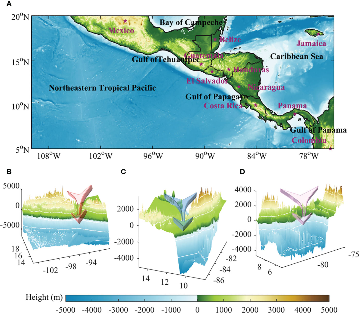
Figure 1 (A) Topography and elevation map of the Northeast Tropical Pacific Ocean and Central America, and (B–D) 3D map of the water depth and coastal land elevation of the Gulf of Tehuantpec, Gulf of Papagayo, and Gulf of Panama, respectively. The color indicates topography (unit: m), the magenta labels and five-pointed stars indicate countries and their capital cities, the black labels indicate the name of the sea (bay), and the arrows in (B–D) indicate the wind direction.

2 Data and methods

This work uses eddy datasets, sea surface velocity and wind stress data. Wind stress and sea surface velocity are used to calculate wind stress work and wind stress curl, while eddy datasets are used to estimate wind stress work and wind stress curl on the eddies.

The satellite altimetry data is produced by Ssalto/Duacs and formerly distributed by Aviso+ with support from CNES/CLS (now distributed by Copernicus Marine and Environment Monitoring Service, https://cds.climate.copernicus.eu), which is the most frequently utilized altimeter data in ocean research. The data is used to calculate the geostrophic velocity from sea level anomalies (SLA). The geostrophic velocity data used in this research have a horizontal grid resolution of 1/4° by 1/4°, a time resolution of 1 day, and a time range of 2000 to 2021.

Gridded daily QuikSCAT and ASCAT scatter-meter wind stress fields are provided by National Oceanic and Atmospheric Administration/National Environmental Satellite Data and Information Service (https://manati.star.nesdis.noaa.gov/products/). Both data have a spatial resolution of 0.25° and a temporal resolution of 1 day, with the former covering the years 2000 to 2008 and the latter covering the years 2009 to 2021.

The eddy data is obtained from the Global Ocean Mesoscale Eddy Atmospheric Biological Interaction Observation Data Set (GOMEAD), which is one of the most widely used in mesoscale oceanic research (Dong et al., 2021; Dong et al., 2022). Using an automatic eddy detection algorithm to obtain parameters of global oceanic mesoscale eddies since 1993, such as polarity, central longitude and latitude, shape, size, and lifecycle. It has a daily resolution and a spatial resolution of 0.15°. The dataset can be acquired from https://dx.doi.org/10.11922/sciencedb.01190.

A total of 114,961 cyclonic eddies and 112,950 anticyclonic eddies from 2000 to 2021 generated in the NETP sea area are identified in the GOMEAD dataset. The calculation formula for work done is as follows:

$$\text{Power}=\overrightarrow{\text{τ}}·\overrightarrow{\text{V}}$$

where $\overrightarrow{\text{τ}}$ is the wind stress, and $\overrightarrow{\text{V}}$ is the oceanic current velocity.

The calculation of wind stress curl uses the curl calculation formula, as shown below:

$$\text{curl}\overrightarrow{\text{τ}}=\frac{\partial {\tau }_y}{\partial x}-\frac{\partial {\tau }_x}{\partial y}$$

where ${\tau }_x$ and ${\tau }_y$ are the zonal component and meridional component, respectively.

The method for configuring variables within the eddy shape: The GOMEAD dataset provides eddy information, including the center and boundary position (shape) of daily eddies. Based on the boundary position information of each eddy, it is determined whether the spatial grid points are within the eddy boundary. The eddy velocity and wind stress values of the grid points included in the eddy boundary position are retained, and the physical values of the grid points not included in the eddy shape are set to null values. Finally, the daily spatial distribution within the eddies shapes is obtained.

The calculation method for the monthly average spatial distribution: Based on the spatial distribution of all days obtained by configuring variables within the eddies shapes, the results of all dates in 12 months are averaged sequentially to obtain the monthly average spatial distribution.

The calculation method of time series: based on the spatial distribution of all days, the area integration is performed to obtain the daily total value, and the results of all dates of each month are averaged to obtain the monthly average.

3 Results

The unique physical surroundings and location of the central America isthmus create ideal circumstances for the formation of wind jets in NETP. Since NETP is situated in the northeast trade wind zone, it is continually impacted by northeast trade winds from the Caribbean and the Gulf of Mexico, particularly the three wind jets that are strongly regulated across the Gulfs of Tehuantpec (TT), Papagayo (PP), and Panama (PN) (Schultz et al., 1998; Chelton et al., 2000). The seasonal average observations of sea surface wind stress and wind stress curl from January 2000 to December 2021 are shown in Figure 2. Consistent with the seasonal variation of wind jets (Xie et al., 2005), wind stress is strongest in winter, followed by transitional periods in spring and autumn, and weakest or even disappears in summer. In the TT and PP, the wind stress is largest at the outlet of the valley and rapidly reduces on both sides. As a result, the positive (negative) wind stress curl is formed along the left (right) side of the wind stress. The wind stress curl in these two sea areas is significantly stronger than that in the surrounding sea areas.

FIGURE 2

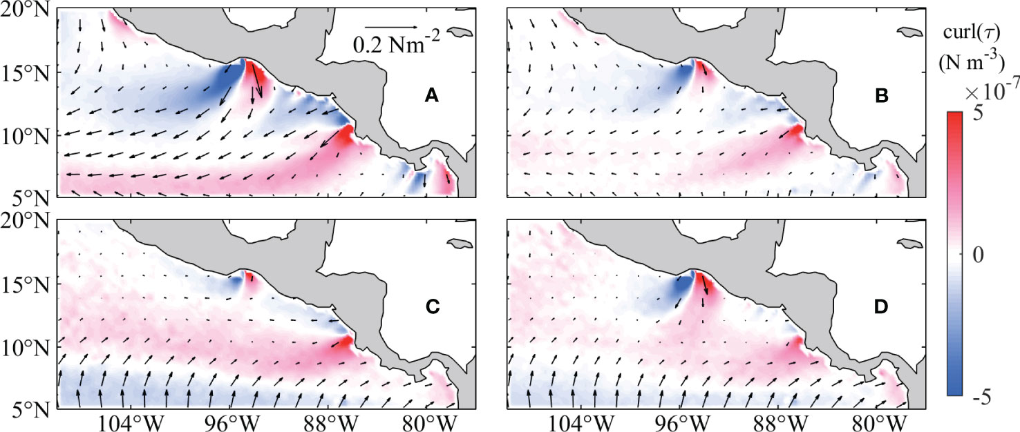
Figure 2 Seasonal variations in average wind stress and wind stress curl from 2000 to 2021. (A) Winter (December to February); (B) Spring (March to May); (C) Summer (June to August); (D) Autumn (September to November). The background color indicates the wind stress curl and the vectors indicate the wind stress.

These strong atmospheric factors force oceanic responses in TT and PP (Mccreary et al., 1989; Barton et al., 1993; Trasviña et al., 1995). A large number of eddies are formed in TT, PP, and PN (Figure 3), which is consistent with previous studies (Hansen and Maul, 1991; Müller-Karger and Fuentes-Yaco, 2000; Gonzalez-Silvera et al., 2004). The spatial distribution characteristics of wind stress and eddy formation are substantially consistent. In addition, wind stress curl is also significantly stronger in these two sea areas than in other regions. In this region, there might be a connection between wind stress curl and eddy generation.

FIGURE 3

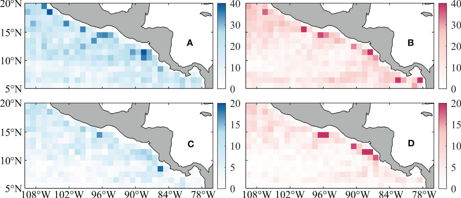
Figure 3 Distribution of eddy generation number. The distributions of generation numbers of cyclonic (left panels) and anticyclonic (right panels) eddies with a life cycle longer than one week are shown in (A) and (B), and those with a life cycle longer than four weeks are shown in (C) and (D). We divided the research area into 1° × 1° boxes for statistics.

To make the comparison between the wind work by relative wind stress and absolute wind stress on oceanic eddies, we conduct a comparison experiment (not shown) and find that the difference between the two types of the wind work is small due to the strong wind speed in the area. Therefore, the absolute wind stress provided by satellite data is used in the following results.

3.1 Time variation of work done by wind stress on eddies

Figure 4 shows the monthly average time series of the wind work, wind stress, and wind stress curl over all eddies in the NETP. The results demonstrate a strong seasonal variation characteristic of the work done by wind stress on eddies in this sea area. The maximum seasonal wind stress work changes on anticyclonic (cyclonic) eddies, wind stress curl changes, and wind stress changes is about 3-3.5 GW (1-1.5 GW, GW = 10⁹ W), 9.5 × 10⁴ N m^-1 (6 × 10⁴ N m^-1) and 5 × 10¹⁰ N (4 × 10¹⁰ N), indicating that the seasonal variation of anticyclonic eddies is more intense. It should be noted that there is a strong connection between wind work and wind stress curl. There is a strong negative correlation between the wind stress curl and wind stress work over anticyclonic eddies, with a correlation as high as -0.906. Instead, there is a positive correlation between wind stress curl and the wind work over cyclonic eddies, with a correlation as high as 0.839. But the correlation between the magnitude of wind stress and the work done by wind stress on eddies is relatively poor (only 0.2~0.3), even though the work done is directly determined by wind stress. This indicates that it is inaccurate to calculate the air-sea momentum flux by only considering the magnitude of wind stress and ignoring the spatial variation of wind stress and the structure of eddies. The comparison between cyclonic eddies and anticyclonic eddies shows that the wind stress curls acting on them are slightly different. The wind stress curls acting on cyclonic eddies tend to have a positive value greater than a negative value and often appear extremely high in summer. In contrast, the wind stress curl acting on anticyclonic eddies has a negative value slightly greater than the positive value. The work done by the wind stress on the anticyclonic eddies is much greater than that on the cyclonic eddies. So, whether the total work done by the wind stress on eddies in this sea area is positive or negative depends on whether the amount of work done by the wind stress on anticyclonic eddies is positive or negative. The average results of anticyclonic and cyclonic eddies for various variables are shown in Table 1. The work done by wind stress on anticyclonic eddies is substantially more than that of cyclonic eddies, even though the wind stress curl operating on anticyclonic eddies is only slightly larger than that of cyclonic eddies. According to Table 1, the average size of cyclonic eddies is similar to that of anticyclonic eddies, however, the average wind power on cyclonic eddies is much less than that of anticyclonic eddies. From the time series of the wind power presented in Figures 4, 5, the wind power on the cyclonic eddies is one magnitude smaller than that on anticyclonic eddies. Therefore, the average wind power on cyclonic eddies is much smaller than that on anticyclonic eddies. This is caused by a few reasons: (1) the average area of cyclonic eddies is about 35% smaller than that of anticyclonic eddies; (2) wind stress over the cyclonic eddies is about 30% smaller than that of anticyclonic eddies; (3) the averaged intensity of velocities in cyclonic eddies is about 96% smaller than that in anticyclonic eddies; (4) cyclonic eddies are prone to highly temporal variation, which causes the smaller averaged wind power. The overall wind stress work is determined to be positive for both anticyclonic and cyclonic eddies based on the average statistical results of wind stress work magnitude across the whole time series.

FIGURE 4

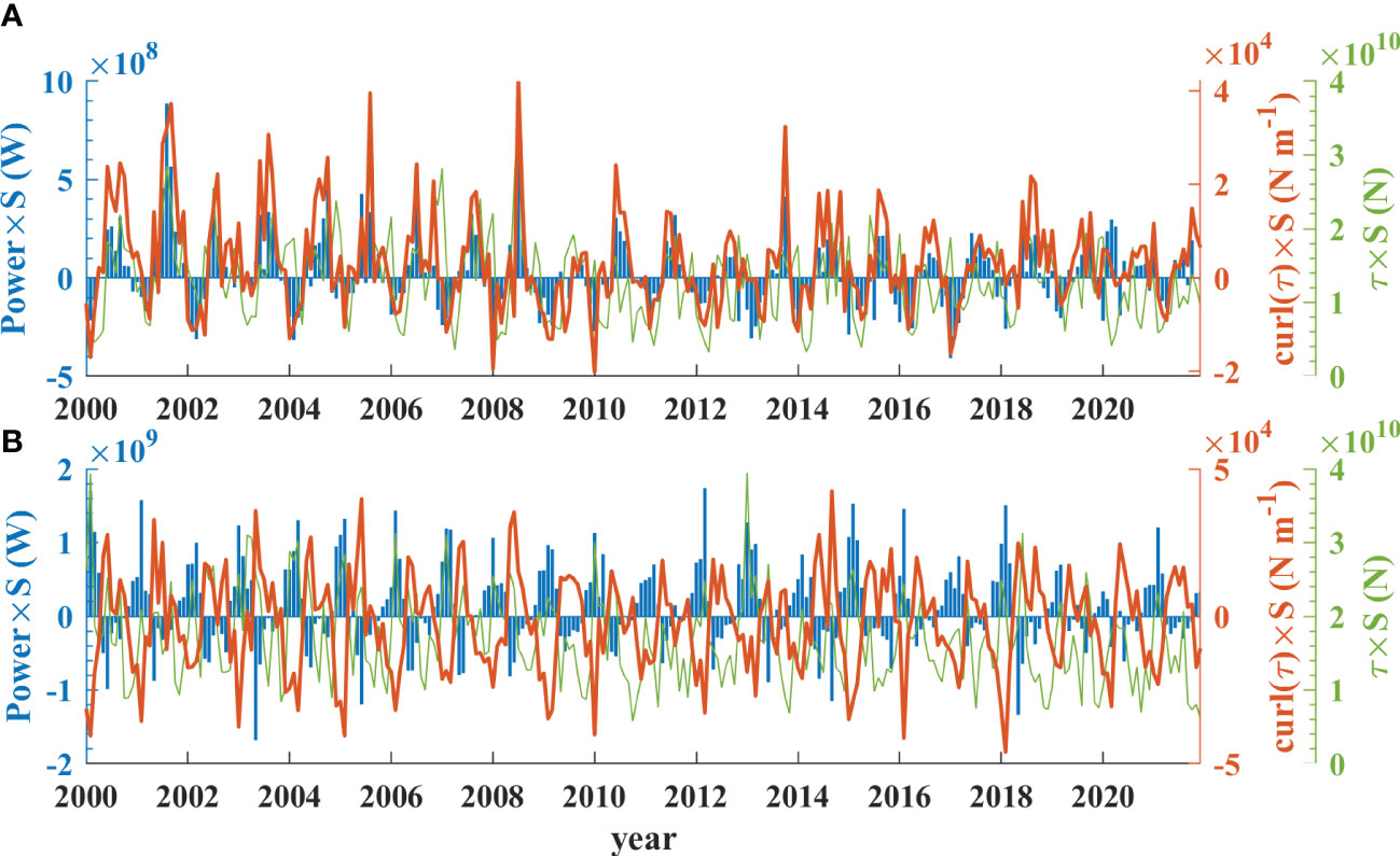
Figure 4 Time series of monthly averaged wind stress work (power; blue bars), wind stress magnitude (τ; green line), and wind stress curl (curlτ; orange line) on (A) cyclonic eddy and (B) anticyclonic eddy. The monthly average is obtained by averaging the results of the daily area integration of all the cyclonic and anticyclonic eddies in the NETP. S represents the area. The correlation coefficient between work done by wind stress on cyclonic eddies and wind stress curl and wind stress magnitude are 0.839 and 0.347, respectively. The correlation coefficient between work done by wind stress on anticyclonic eddies and wind stress curl and wind stress magnitude are -0.906 and 0.237, respectively.

TABLE 1

Table 1 Averaged results from 2000 to 2021.

FIGURE 5

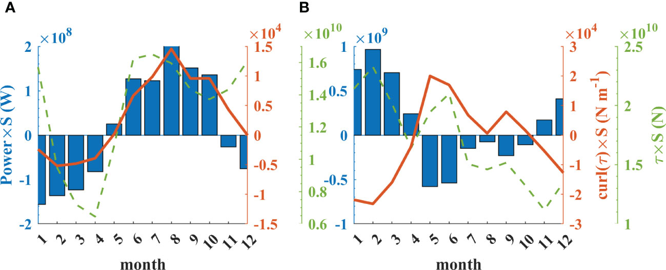
Figure 5 Annual cycle of wind stress work (power; blue bars), wind stress curl (curlτ; orange line), and wind stress magnitude (τ; green line) during 2000-2021 average over the study area. (A) Cyclonic eddies, and (B) anticyclonic eddies. S is the area.

The multi-year monthly average wind stress work on eddies, wind stress curl, and wind stress magnitude are presented in Figure 5 to better illustrate the seasonal characteristics of wind stress work on eddies. For cyclonic eddies, the work done by wind stress is most negative in January, gradually increases to the most positive value from January to August, and then gradually decreases to negative values from August to December. Similar to the work done by the wind stress on the cyclonic eddies, the wind stress curl acting on the cyclonic eddies exhibits seasonal variation. Compared to wind stress work and wind stress curl, the variation in the strength of the wind stress acting on a cyclonic eddy is noticeably different. There are considerable seasonal fluctuations in both the wind stress work and curl acting on the anticyclonic eddies. From January to March, the wind stress has a significant positive work on the anticyclonic eddy, which remains positive in April but sharply decreases to the most negative value in May. A sharp increase occurs from June to August, with a slight negative rebound in September and a steady growth from October to December. It is opposite to the positive and negative values of cyclonic eddies, being positive from January to April, November to December, and negative from May to October. It can be seen that work done by wind stress on cyclonic and anticyclonic eddies has completely different seasonal variation characteristics.

Overall, the averaged wind stress curl over cyclonic eddies is negative in winter and positive in summer, and the averaged wind work on cyclonic eddies is negative in winter and positive in summer, which shows a positive correlation between the wind stress curl and the wind work. For anticyclonic eddies, such correlation is negative.

3.2 Spatial distribution of work done by wind stress on eddies

The monthly average spatial distribution of the work done by wind stress on anticyclonic and cyclonic eddies from 2000 to 2021 is shown in Figures 6, 7, respectively. Overall, the intensity of wind work over anticyclonic eddies is significantly stronger than that over cyclonic eddies, and its seasonal variation characteristics are more obvious.

FIGURE 6

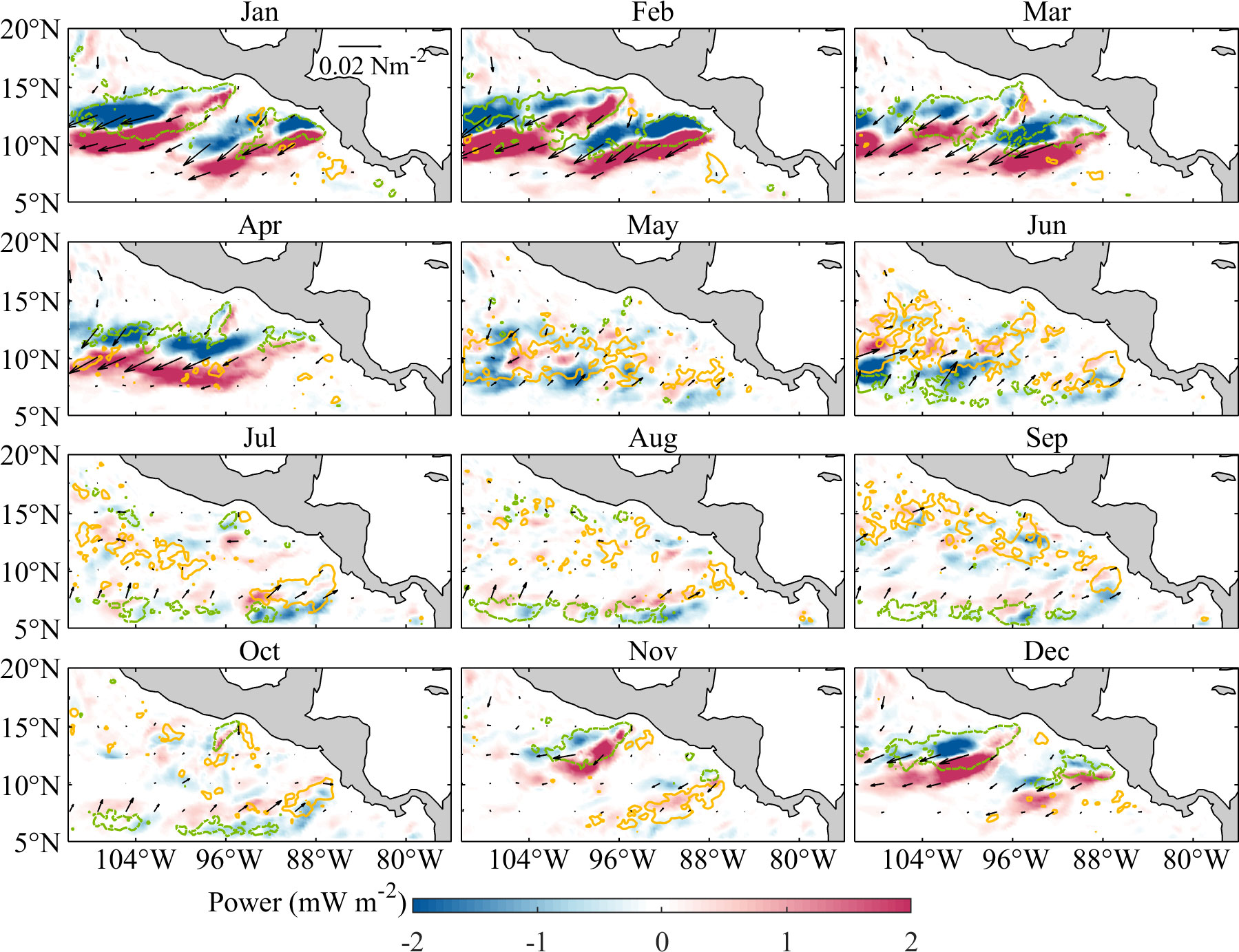
Figure 6 Monthly distribution of wind stress work on anticyclonic eddies during 2000-2021 derived from altimeter and scatterometer data. The color shading indicates the work done (Power, mW m^-2 = 10^-3 W m^-2) by wind stress on the anticyclonic eddies, and yellow and green lines represent the wind stress curl isolines of 2 × 10^-8, -2 × 10^-8 N m^-3, respectively, with the black vectors indicating wind stress.

FIGURE 7

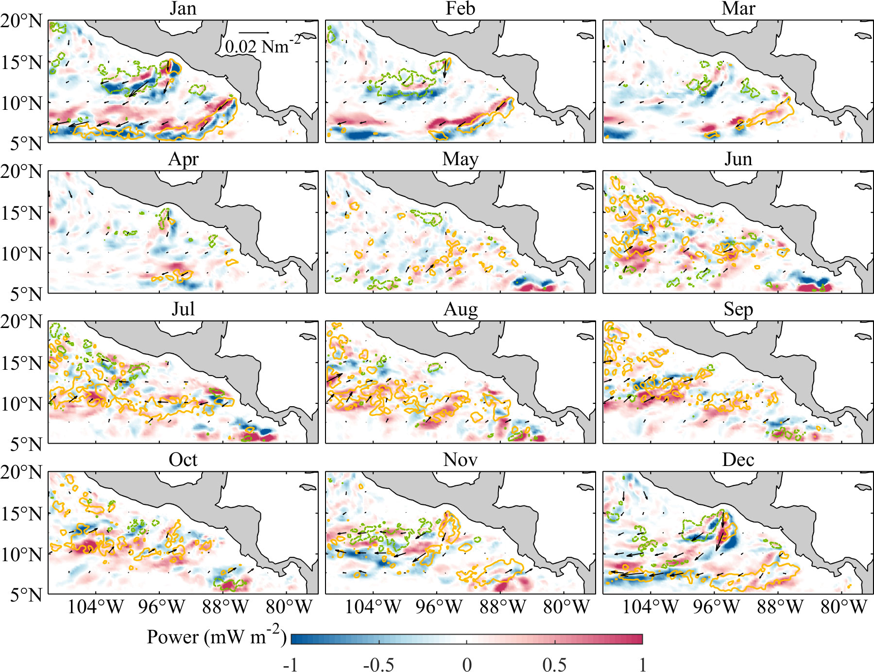
Figure 7 Same as Figure 6, but for cyclonic eddies.

The wind stress works on the anticyclonic eddy shows two groups of significant north-negative south-positive long stripes distributed near TT and PP sea areas and extending to the southwest from January to April. Regions with positive wind power slightly greater than regions with negative wind power. The wind stress acting over anticyclonic eddies is mainly in the northeast where with large negative wind stress curl. The wind stress work decreases since May, the wind stress over anticyclonic eddies transfers to northeast to southwest, and the wind stress curl is mainly positive. From November, the positive distribution of wind stress work is slightly larger than the negative distribution, and the wind stress increase and wind stress curl to become negative.

For cyclonic eddies, the wind power from January to March is distributed along the high wind stress areas near TT and PP and their extending towards the southwest, presenting a discontinuous north-south distribution, which gradually declines and disappears completely in April. At this time, the predominant wind stress curl distribution in TT and PP is opposite. While the wind stress curls in PP are primarily positive and the positive distribution of wind stress work on the eddy is greater than the negative distribution, the wind stress curls in TT are primarily negative. Only a stronger north-negative south-positive short strip appears in the region west of PN during April and May, with weak work done noted over the rest of the area. Throughout July to October, there is a sizable distribution of wind stress work between 95° and 110°, which coincides with the large distribution of positive wind stress curl at that time, mostly doing positive work on eddies. Positive and negative wind stress curls are equal in November and both positive and negative work done by wind stress on the eddies are similar. The negative wind stress curl is substantial in December, and the work done by wind stress on cyclonic eddies is primarily negative.

In general, the wind stress curl distribution matches the work done by wind stress on cyclonic and anticyclonic eddies. Specifically, where the wind stress curl is negative (positive), the wind stress generally does positive (negative) work on the anticyclonic eddy. The wind stress primarily does positive (negative) work on cyclonic eddies in regions where the wind stress curl is positive (negative).

Owing to the symmetrical and opposing flow field structure distribution of eddies, when wind stress acts on them, it is evident that one side of the flow velocity direction is in the same direction as the wind stress while the other side is in the opposite direction to the wind stress. Positive work occurs on the side flowing in the same direction as the wind stress, whereas negative work occurs on the opposing side. As a result, positive and negative work frequently occur concurrently. The work done by wind stress on an eddy that can live for tens to hundreds of days appears as a continuous strip that tracks the eddy’s movement. Therefore, the distribution of work done by wind stress on the eddy is often closely related to the movement trajectory of the eddy, especially for eddies with long lifespans. Long-live eddies often carry greater energy, have greater size and flow velocity, and wind stress does more work on them. The tracks of such eddies are depicted in Figure 8. It is found that there are significant differences in the number, formation and distribution of long-live cyclonic and anticyclonic eddies. The number of long-live anticyclonic eddies is significantly greater than that of cyclonic eddies, and their propagation distance is much farther than that of cyclonic eddies. Long-live anticyclonic eddies are mostly generated in TT and PP. TT-generated anticyclonic eddies propagate southwest for hundreds of kilometers fairly consistently, whereas PP-generated anticyclonic eddies first move slightly north and then turn southwest to exit. Cyclonic eddies are scattered throughout the coastal area and open ocean, primarily traveling west or northwest. This is because the movement of eddies mostly depends on the β-effect and advection of the background flow field, which causes cyclonic eddies to travel mostly toward the poles, while anticyclonic eddies move toward the equator (Mcwilliams and Flierl, 1979; Chelton et al., 2011). The high-value wind stress coincides with the movement trajectory of the long-live anticyclonic eddy, resulting in a clear work done striped distribution. Unfortunately, the movement path of cyclonic eddies does not match the high wind stress, and their life cycle is short. As a result, only a limited amount of work is accumulated, and a continuous distribution is impossible.

FIGURE 8

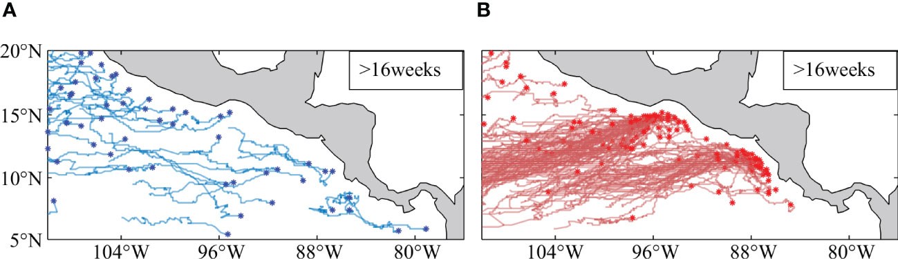
Figure 8 Propagation trajectories of (A) cyclonic eddies and (B) anticyclonic eddies with more than 16 weeks lifespan. The asterisk represents the eddy generation location, while the curve reflects its migration trajectory.

3.3 Case studies of wind stress doing work on eddy

Considering that process information may be masked by average results, eddy cases are selected for analysis. The selected examples below illustrate the relationship between wind stress work and wind stress curl during the full life cycle of the eddies.

3.3.1 Case study of an anticyclonic eddy

This anticyclonic eddy has a lifespan of 188 days, forming on February 27 and disappearing on September 4, 2002. It formed in TT where wind stress curl is negative (see Figure 9A). Its radius was initially small, but as it developed towards the southwest, its size gradually increased. From April to June, the size reaches a maximum between 100° W to 103° W and 10° N, and then the eddy gradually shrinks and disappears. The average radius of eddies during their life cycle is 151.68 km.

FIGURE 9

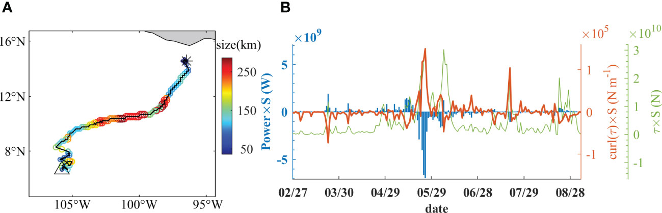
Figure 9 (A)Trajectory of the anticyclonic eddy case. It formed on February 27 and disappeared on September 4, 2002. The solid black line represents the center trajectory of the anticyclonic eddy, and the color of the circles represent the size of the anticyclonic eddy. (B) Time series of work done by the wind stress on the eddy (power; blue bars), wind stress curl acting on the eddy (curlτ; orange line) and magnitude of the wind stress (τ; green line) for the anticyclonic eddy case. Each item is a daily area (S) integration result within the eddy.

Figure 9B shows the wind stress work done on the eddy, the wind stress curl and the wind stress magnitude. The wind stress curl acting on the anticyclonic eddy is primarily negative from February to April, and the wind stress work exhibits mainly positive values. From late May to early June, the wind stress curl changes to a positive value, and the wind stress work exhibits primarily negative values. Both wind stress curl and wind stress work have very big values due to the increase in eddy size. After mid-June, the wind stress curl and the wind stress work exhibit alternate positive and negative values, but both are extremely low since the eddy size decreases.

Figure 10 shows the spatial distribution of the anticyclonic eddy case, with a few typical moments chosen for examination. From February to April 5, the anticyclonic eddy is primarily subject to negative wind stress curl from a northeast wind action in TT. The positive work done by the wind stress is significantly higher than the negative work done, i.e., the work done in the northwest is positive, while the work done in the southeast is negative. On April 6, most locations experience positive wind stress curls, with the positive work component weakening and the negative work component strengthening. On April 7, most regions have negative wind stress curls, with the wind stress’ positive work component strengthening and its negative work component weakening. On April 12, the wind stress curl turns positive once more, the positive work weakens, and the negative work strengthens again. There is a phenomenon of alternating positive and negative power during the later stage of the eddy life cycle, such as on April 14 and May 1. Up until May 21st, there is a very strong spatial variation in wind stress with a scale similar to an anticyclonic eddy and its direction completely opposite that of an anticyclonic eddy, that is, a cyclonic distribution above the entire anticyclonic eddy. Thus the negative work almost completely covers the anticyclonic eddy. On May 22, the strong wind stress direction flips in the south, causing the work done on the eddy by wind stress to change to a very strong positive value. From May 23rd to 25th, the wind stress acts on the anticyclonic eddy in a cyclonic manner at the scale of the eddy, and its spatial variation scale is similar to the scale of the eddy, forming a strong wind stress curl. In most regions, the wind stress work is significantly negative. In contrast to the distribution in March, the wind stress operating over the anticyclonic eddy changes to a southwest direction starting in June. As a result, the wind stress does positive work on the anticyclonic eddy’s northwest part and negative work on its southeast part.

FIGURE 10

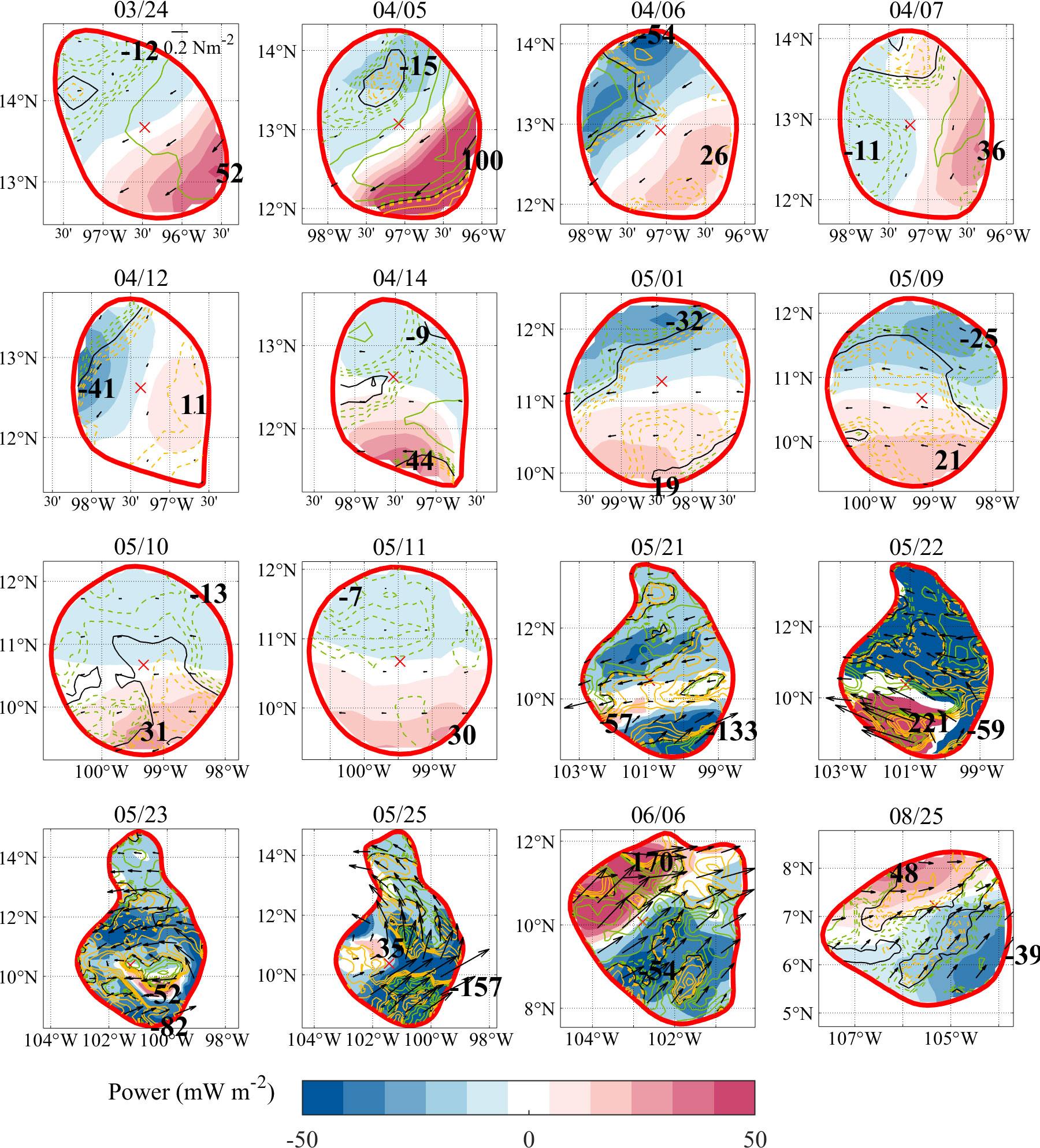
Figure 10 Spatial distribution of the anticyclonic eddy case. The background color indicates the work done by the wind stress on the eddy. The numbers represent the maximum and minimum work done (marked near the location where it occurs). The red circle indicates the shapes boundary of the anticyclonic eddy, the red × represents the center of the anticyclonic eddy, the black arrow represents the wind stress, and the yellow (green) solid line represents the positive (negative) wind stress curl isolines, with a value of 5×10^-7, 1×10^-6, 1.5×10^-6 (-5×10^-7, -1×10^-6, -1.5×10^-6) N m^-3, yellow (green) dotted lines represent smaller positive (negative) wind stress curl isolines, spaced at 5×10^-8, 1×10^-7, 1.5×10^-7 (-5×10^-8, -1×10^-7, -1.5×10^-7) N m^-3.

3.3.2 Case study of a cyclonic eddy

The cyclonic eddy persisted for 35 days, forming on November 18 and decaying on December 22, 2013. It developed where there is a positive wind stress curl in TT (see Figure 11A). Its size is initially small but progressively grows and eventually stays at 60~70 km as it proceeds northwest. Ultimately, the eddy gradually shrinks in size and vanishes. Its average radius during its whole life cycle is 58.13 km.

FIGURE 11

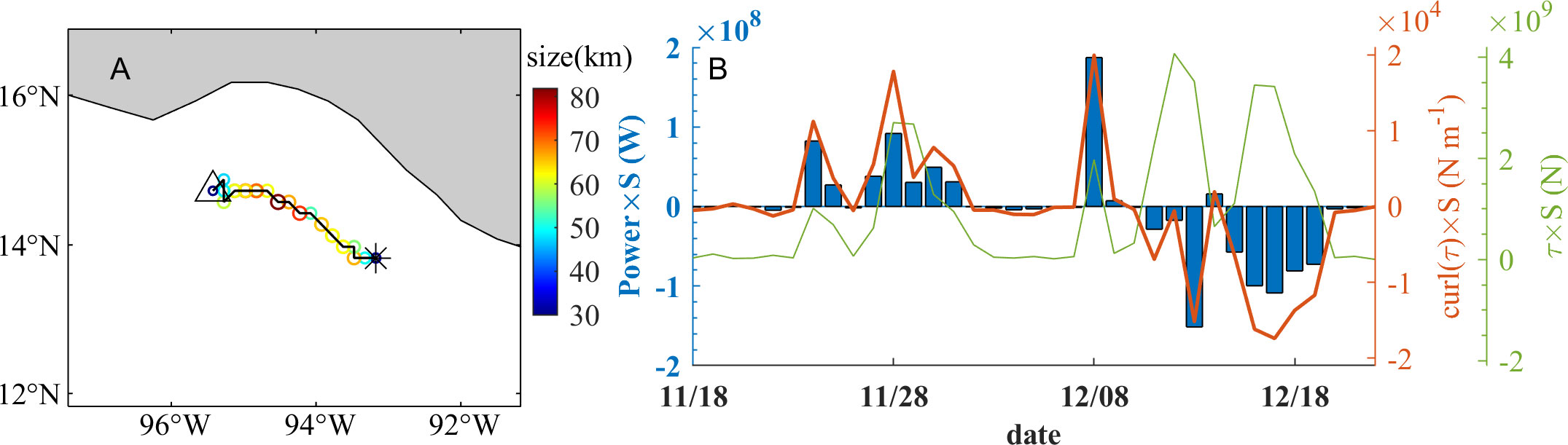
Figure 11 (A) Trajectory of the cyclonic eddy case. It formed on November 18 and disappeared on December 22, 2013. The solid black line represents the center trajectory of the cyclonic eddy, and the color of the circles represents the size of the cyclonic eddy. (B) Time series of work done by the wind stress on the eddy (power; blue bars), wind stress curl acting on the eddy (curlt; orange line) and magnitude of the wind stress (t; green line) for the cyclonic eddy case. Each item is a daily area (S) integration result within the eddy.

Figure 11B displays the cyclonic eddy’s time series. During the early stage, the wind stress work done is generally positive, while the wind stress curl acting on the cyclonic eddy is primarily negative. The amplitude of wind stress diminishes in early December, the overall wind stress curl is very small, and the work done is insignificant. By December 8, the wind stress curl and the wind stress work are highly positive values. Both the wind stress curl and the wind stress work on the eddy are extremely high due to the eddy size increasing. The cyclonic eddy finally moves into an area where the wind stress curl is very negative in the middle and late stages. As a result, both the wind stress curl and the wind stress work are negative.

The spatial distribution of the cyclonic eddy is displayed in Figure 12, and certain typical moments are chosen for examination. The wind stress curl acting on the cyclonic eddy is mainly positive from November 24 to November 28. The wind stress originates from the influence of the north wind in TT. The positive part of the wind stress work in the same direction as the eddy rotation is significantly more than the negative part in the opposite direction. The negative work area grows on November 29th, but positive work is generally still observed despite the negative wind stress curl. Between November 30 and December 7, the wind stress steadily decreases, followed by a reduction in the work done and the wind stress curl. By December 8, the wind stress grows, particularly in the western side of the eddy facing the same direction and the wind stress curl increases to positive values. It is substantially bigger on the western side, where positive work is done, than on the east with negative work. Wind stress has a beneficial effect on the entire eddy. The wind stress curl covering the eddy changes to negative during the following few days as it moves to an area where the wind stress curl is negative. The amount of wind stress that causes negative work on the eddy is noticeably greater than that of positive work. Therefore, the wind stress causes negative work done on the entire eddy at this time.

FIGURE 12

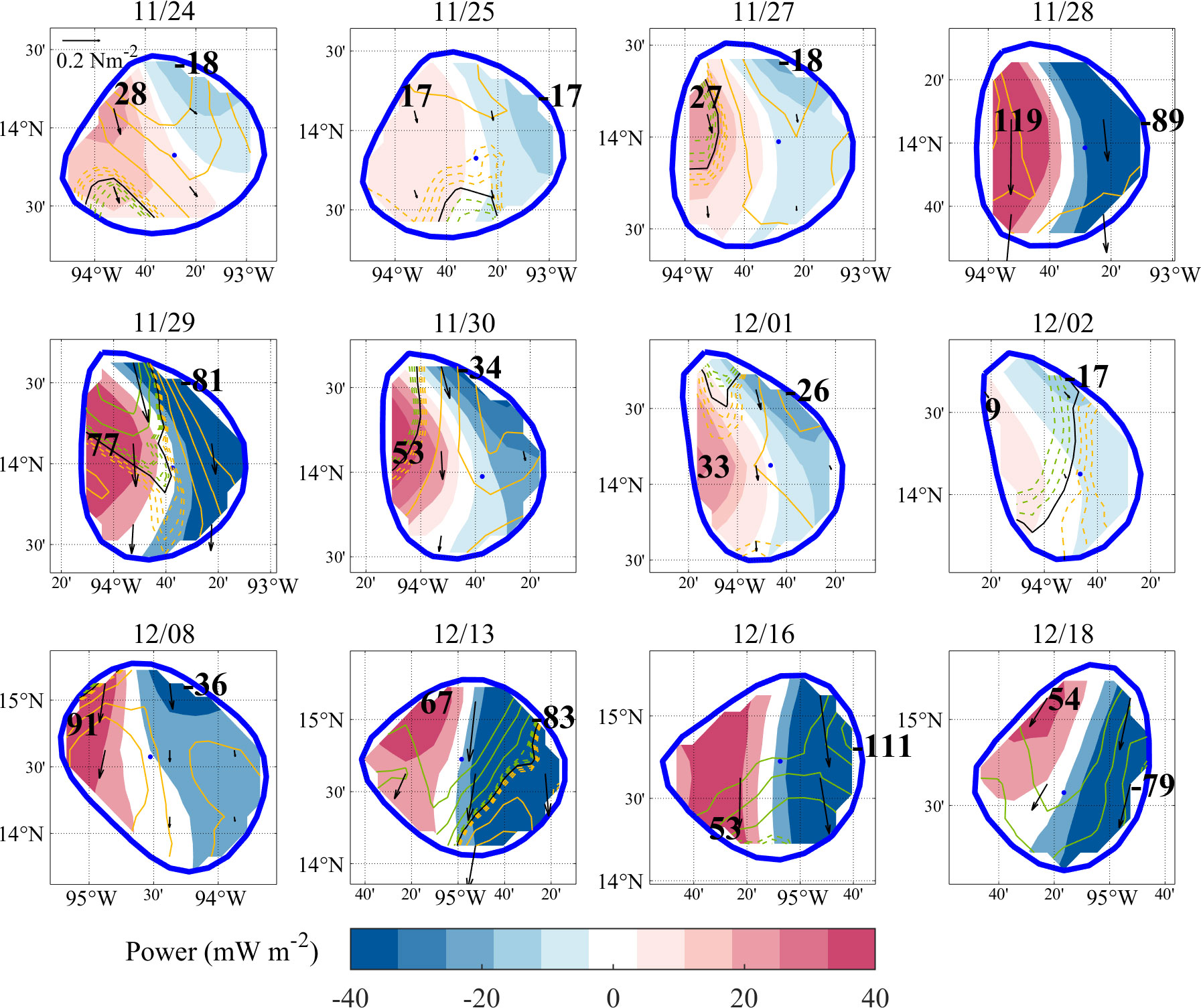
Figure 12 Same as Figure 10, but for the cyclonic eddy case and the blue circle indicates the shapes boundary of the cyclonic eddy, the blue • represents the center of the cyclonic eddy.

If we decompose the wind stress into the uniform spatial distribution of the wind stress (averaged over the eddy field) and deviation from the uniform wind stress, one can see that the contribution by the net wind power is mainly caused by the deviation part.

3.4 Mechanism of wind stress acting on eddy

Based on the results above, we can summarize the mechanism of wind stress acting on eddies under different wind stress curl conditions using a schematic diagram (Figure 13). Here, it is assumed that the ideal eddy has a symmetric flow velocity distribution and different spatial distributions of wind stress acting on the eddy. At first, a symmetrical distribution of wind stress is created based on the features of wind stress distribution in TT and PP. The direction of the distribution is from east to west, and the magnitude of the distribution gradually increases to the maximum value from north to south before gradually decreasing, generating a distribution of negative wind stress curl in the northern half and positive wind stress curl in the southern half. The work done by four types of wind stresses with different rotations on anticyclonic and cyclonic eddies is discussed. The wind stress curl in (A-B) is less negative, the wind stress curl in (C-D) is less positive, while the wind stress curl in (E) is more negative, and the wind stress curl in (f) is more positive. Since the v-component is perpendicular to the wind stress, they are multiplied by 0, so only the u-component is considered. At the same time, since it is assumed that the flow velocity u-component of an ideal eddy is equal at the north and south and opposite in direction, the magnitude of the wind stress work done on the northern and southern parts of the eddy depends on the magnitude of the wind stress on each side.

FIGURE 13

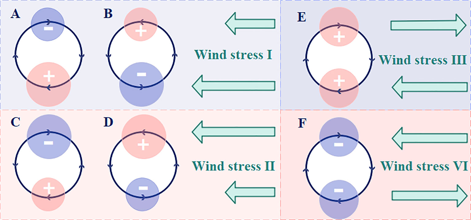
Figure 13 Schematic diagram of wind stress work done on eddies. Anticyclonic eddies (A) and cyclonic eddies (B) are affected by wind stress with minor negative vorticity, whereas wind stress with modest positive vorticity acts on anticyclonic eddies (C) and cyclonic eddies (D). The anticyclonic eddy is affected by the wind stress with positive rotation and negative rotation, whose spatial variation scale corresponds to the eddy scale (i.e., strong). The green arrow indicates the magnitude and direction of wind stress, the dark blue closed curve in (A–F) represents a standard eddy, the dark blue arrow represents the rotation direction of the eddy, the (clockwise) counterclockwise rotation represents (anti) cyclonic eddy, the blue (pink) circle inside the eddy represents the negative (positive) work done by the wind stress on the eddy, the size of the circle represents the relative magnitude of positive and negative work done, and the background color represents the magnitude of wind stress curl, the light red (blue) background represents positive (negative) wind stress curl, and the relative darkness of the background colors of (A–D) and (E, F) represents the relative magnitude of curl.

Under the action of wind stress with mild vorticity, anticyclonic (A, C) and cyclonic eddies (B, D) present wind stress work that is stronger on the side with more wind stress and weaker on the other side. The relative direction between the wind stress and eddy flow velocity determines whether the wind work is positive or negative. In (A), the anticyclonic eddy’s velocity u-component on the southern (northern) side is parallel to (opposite to) the wind stress direction. The magnitude of the wind stress on the southern side is greater than that on the northern side, and the wind stress does positive work (negative work) on the southern (northern) side. As a result, for this anticyclonic eddy, the positive work on the southern side outweighs the negative work which is lost on the northern side, and the wind stress contributes positively to the outcome of its entire activity. As an illustration, considering the anticyclonic eddy from March 24 to April 5, April 7, April 14, and May 10-11, 2002, the north-south distribution is deflected according to the direction of wind stress. In (B), the flow velocity u-component is opposite (similar) to the direction of the wind stress on the southern (northern) side of the cyclonic eddy. The magnitude of the wind stress on the southern side is greater than that on the northern side at this time, and the wind stress does negative work (positive work) on the southern (northern) side. Therefore, for this cyclonic eddy, the negative work lost on the southern side is greater than the positive work on the northern side, and the wind stress contributes negatively to its overall action result. For example, this occurs from December 13 to 18, 2013 (the north-south distribution is distorted according to the direction of wind stress, approaching an east-west distribution where the wind stress rotates counterclockwise by 90°). Since the wind stress for (C) and (D) is larger in the north than in the south, their work on anticyclonic (C) and cyclonic eddies (D) are of greater magnitude in the north than in the south. The positive and negative effects of wind stress on anticyclonic and cyclonic eddies are still negative in the north while positive in the south and positive in the north while negative in the south, respectively, since the wind direction from east to west remains unchanged. Therefore, for the anticyclonic eddy (C), the negative work lost on the northern side is greater than the positive work on the southern side, and the wind stress has a negative contribution to its overall effect, corresponding to the anticyclonic eddy case on April 6, April 12, May 1, and May 9, 2022. In contrast, the positive work on the northern side of cyclonic eddy (D) exceeds the negative work lost on the southern side, and the wind stress contributes positively to its total action, corresponding to the situation of the cyclonic eddy case on November 24, November 27-28, November 30-December 1, and December 8, 2013.

The wind stress curl may be very significant in extreme circumstances. Therefore, a set of cases where the spatial variation scale of wind stress is equivalent to the scale of anticyclonic eddies is designed. Namely, the work situation under the condition that the wind stress curl is a large negative curl (E) and the wind stress curl is a large positive curl (F). In (E), it is clear that the wind stress has a favorable effect on the entire anticyclonic eddy because it is consistent with the anticyclonic eddy flow direction on both the northern and southern sides. In (F), the wind stress acts negatively on the entire anticyclonic eddy since it is contrary to the anticyclonic eddy flow velocity direction on both the northern and southern sides. In the actual ocean, there are not many perfect extreme situations. However, the anticyclonic eddy on May 21 and May 23~25, 2002, can essentially show this circumstance. For cyclonic eddies, there can also be situations where the wind stress curl is extremely large. Although if it is not depicted in this example, the fundamental requirement is still the of the eddy’s flow velocity direction and the wind stress. When the wind stress curl and the eddy are in the same direction, the wind stress produces positive work on the entire eddy, and vice versa.

4 Discussion

It is clear from the two examples in Section 3.4 that changes in the wind stress curl significantly impact wind stress work. While having different polarities, cyclonic and anticyclonic eddies share many characteristics. At the beginning of their life cycles, they are both found in locations with the same polarity as the wind stress curl. During this period, wind stress does positive work on them. In the latter stages, as they move into regions with opposite wind stress curls polarity, the wind stress does negative work on them. Wind stress and wind stress curl are potential eddy generation mechanisms in the TT and PP zones. (Liang et al., 2012). Because wind stress (curl)-generated eddies have the same polarity as the wind stress curl, it can be said that wind stress is likely to positively affect the eddy’s early life cycle. This can explain the significant positive value of wind stress work on eddies in the NETP. A lot of eddies with the same polarity as the wind stress curls are generated as a result of the strong wind stress curls in NETP, meaning that wind stress has a positive effect on these eddies.

This occurrence is not limited to the NETP region. Wind stress is a significant mechanism for the development of local eddies in the leeward parts of Hawaii Island and the eastern South China Sea (Wang et al., 2008; Jia et al., 2011; Wang et al., 2012). There are also major positive phenomena of wind stress work done on eddies in these locations based on the global distribution of wind stress work done in previous studies (Xu et al., 2016; Rai et al., 2021).

In other words, wind stress “kills” the eddy when the eddy structure is independent of the wind field. For instance, front-related baroclinic instability generates eddies in the subtropical frontal region (Kobashi and Kawamura, 2002; Qiu and Chen, 2011), jet instability causes eddy formation in the Kuroshio extension region (Itoh and Yasuda, 2010; Liu et al., 2017), and upwelling front instability causes eddies to form off the coast of California (Dong et al., 2009). These eddies are independent of wind stress forcing and are produced by environmental elements in the ocean’s flow. As a result, the wind stress does negative work on the eddies due to the mismatch between the rotational direction of the eddy and the direction of the wind stress.

5 Conclusions

Most views believe that wind stress “kills” eddies in most oceans, and very few studies focused on the possible positive impact of wind stress on eddies and the dynamic changes in energy input due to wind stress.

This study focuses on the NETP sea area, where there is a considerable positive wind stress work on eddies. The spatiotemporal characteristics of the work done by wind stress on eddies and case studies of wind stress on eddies in the NETP, are studied using 22 years (2000 to 2021) of satellite remote sensing data and eddy data sets. The research results show a significant seasonal variation in the work done by wind stress on eddies in the NETP. Specifically, the overall wind stress work on the (anti) cyclonic eddy is (positive) negative in winter and (negative) positive in summer. The correlation coefficient between wind power and wind stress curl over (anti) cyclonic eddies is (-0.906) 0.839. Their spatial distribution also matches well. Generally, wind stress primarily contributes positively (negatively) to anticyclonic eddies in regions where the wind stress curl is negative (positive). In contrast, wind stress contributes positively (negatively) to cyclonic eddies in regions where the wind stress curl is positive (negative). Case studies reveal that the positive work done by the same polarity of eddy and curl of wind stress, and negative work done by the opposite polarity of eddy and curl of wind stress condition is satisfied by the work done by wind stress on an eddy. At the same time, wind stress affects the eddy positively in the early stages of its life cycle and negatively in the latter stages. This is because the eddy is initially driven by wind stress and its polarity is identical to the wind stress curl. When the eddies later move to an area with an opposite wind stress curl, wind stress starts acting against it.

The present findings, along with results from previous related studies, suggest that the wind energy input is sensitive to the wind stress curl and mesoscale eddy velocity structure. Consequently, it is essential to consider the spatial distribution of wind stress, the unique structure of the eddy, and their temporal variation and regional characteristics, when determining the work done by wind stress on eddies. This study, however, only analyzes the dynamic impact of wind stress on eddies on the sea surface. Many aspects of the ocean are affected by the interaction between wind and eddies, including the thermal effect and the three-dimensional dynamic effect of wind stress on eddies. Further exploration of this topic requires more extensive research, including numerical simulations and field observations, which will be left for future research.

Data availability statement

The original contributions presented in the study are included in the article/supplementary material. Further inquiries can be directed to the corresponding author.

Author contributions

FT, CD, and WZ conceived and designed the experiments. FT performed the experiments. FT analyzed the data. FT drafted the original manuscript. FT, CD, KL and JJ revised and edited the manuscript. All authors contributed to the article and approved the submitted version.

Funding

This research is funded by Jiangsu Natural Resources Development Special Fund (Marine Science and Technology Innovation) (JSZRHYKJ202102) and the National Natural Science Foundation of China (Nos. 42192562, 42250710152).

Acknowledgments

The satellite altimetry data is produced by Ssalto/Duacs and formerly distributed by Aviso+ with support from CNES/CLS (now distributed by Copernicus Marine and Environment Monitoring Service, https://cds.climate.copernicus.eu). Gridded daily QuikSCAT and ASCAT scatter-meter wind stress fields are provided by National Oceanic and Atmospheric Administration/National Environmental Satellite Data and Information Service (https://manati.star.nesdis.noaa.gov/products/). The GOMEAD dataset can be acquired from https://dx.doi.org/10.11922/sciencedb.01190.

Conflict of interest

The authors declare that the research was conducted in the absence of any commercial or financial relationships that could be construed as a potential conflict of interest.

Publisher’s note

All claims expressed in this article are solely those of the authors and do not necessarily represent those of their affiliated organizations, or those of the publisher, the editors and the reviewers. Any product that may be evaluated in this article, or claim that may be made by its manufacturer, is not guaranteed or endorsed by the publisher.

References

Barton E. D., Argote M. L., Brown J., Kosro P. M., Lavin M., Robles J. M., et al. (1993). Supersquirt: dynamics of the gulf of tehuantepec, Mexico. Oceanography 6, 23–30. doi: 10.5670/oceanog.1993.19

CrossRef Full Text | Google Scholar

Chelton D. B., Freilich M. H., Esbensen S. K. (2000). Satellite observations of the wind jets off the pacific coast of central america. part I: case studies and statistical characteristics. Mon. Weather Rev. 128, 1993–2018. doi: 10.1175/1520-0493(2000)128<1993:SOOTWJ>2.0.CO;2

CrossRef Full Text | Google Scholar

Chelton D. B., Schlax M. G., Samelson R. M. (2011). Global observations of nonlinear mesoscale eddies. Prog. Oceanogr. 91, 167–216. doi: 10.1016/j.pocean.2011.01.002

CrossRef Full Text | Google Scholar

Dong C., Idica E. Y., Mcwilliams J. C. (2009). Circulation and multiple-scale variability in the southern California bight. Prog. Oceanogr. 82, 168–190. doi: 10.1016/j.pocean.2009.07.005

CrossRef Full Text | Google Scholar

Dong C., Liu L., Nencioli F., Bethel B. J., Liu Y., Xu G., et al. (2022). The near-global ocean mesoscale eddy atmospheric-oceanic-biological interaction observational dataset. Sci. Data 9, 436. doi: 10.1038/s41597-022-01550-9

PubMed Abstract | CrossRef Full Text | Google Scholar

Dong C., Liu L., Nencioli F., Xu G., Ma J., Ji J., et al. (2021). Global ocean mesoscale eddy atmospheric-Oceanic-Biological interaction observational dataset (GOMEAD)(V1). Sci. Data Bank: Beijing China. doi: 10.11922/sciencedb.01190

CrossRef Full Text | Google Scholar

Duhaut T. H., Straub D. N. (2006). Wind stress dependence on ocean surface velocity: implications for mechanical energy input to ocean circulation. J. Phys. Oceanogr. 36, 202–211. doi: 10.1175/JPO2842.1

CrossRef Full Text | Google Scholar

Gonzalez-Silvera A., Santamaria-Del-Angel E., Millan-Nunez R., Manzo-Monroy H. (2004). Satellite observations of mesoscale eddies in the gulfs of tehuantepec and papagayo (Eastern tropical pacific). Deep Sea Res. Part II 51, 587–600. doi: 10.1016/j.dsr2.2004.05.019

CrossRef Full Text | Google Scholar

Hansen D. V., Maul G. A. (1991). Anticyclonic current rings in the eastern tropical pacific ocean. J. Geophys. Res.: Oceans 96, 6965–6979. doi: 10.1029/91JC00096

CrossRef Full Text | Google Scholar

Huang R. X., Wang W., Liu L. L. (2006). Decadal variability of wind-energy input to the world ocean. Deep Sea Res. Part II 53, 31–41. doi: 10.1016/j.dsr2.2005.11.001

CrossRef Full Text | Google Scholar

Itoh S., Yasuda I. (2010). Characteristics of mesoscale eddies in the kuroshio–oyashio extension region detected from the distribution of the sea surface height anomaly. J. Phys. Oceanogr. 40, 1018–1034. doi: 10.1175/2009JPO4265.1

CrossRef Full Text | Google Scholar

Jia Y., Calil P., Chassignet E., Metzger E., Potemra J., Richards K., et al. (2011). Generation of mesoscale eddies in the lee of the Hawaiian islands. J. Geophys. Res.: Oceans 116, C11009. doi: 10.1029/2011JC007305

CrossRef Full Text | Google Scholar

Kobashi F., Kawamura H. (2002). Seasonal variation and instability nature of the north pacific subtropical countercurrent and the Hawaiian Lee countercurrent. J. Geophys. Res.: Oceans 107, 6–1-6-18. doi: 10.1029/2001JC001225

CrossRef Full Text | Google Scholar

Liang J. H., Mcwilliams J. C., Kurian J., Colas F., Wang P., Uchiyama Y. (2012). Mesoscale variability in the northeastern tropical pacific: forcing mechanisms and eddy properties. J. Geophys. Res.: Oceans 117, C07003. doi: 10.1029/2012JC008008

CrossRef Full Text | Google Scholar

Liu Y., Dong C., Liu X., Dong J. (2017). Antisymmetry of oceanic eddies across the kuroshio over a shelfbreak. Sci. Rep. 7, 6761. doi: 10.1038/s41598-017-07059-1

PubMed Abstract | CrossRef Full Text | Google Scholar

Mccreary J. P., Lee H. S., Enfield D. B. (1989). The response of the coastal ocean to strong offshore winds: with application to circulations in the gulfs of tehuantepec and papagayo. J. Mar. Res. 47, 81–109. doi: 10.1357/002224089785076343

CrossRef Full Text | Google Scholar

Mcwilliams J. C., Flierl G. R. (1979). On the evolution of isolated, nonlinear vortices. J. Phys. Oceanogr. 9, 1155–1182. doi: 10.1175/1520-0485(1979)009<1155:OTEOIN>2.0.CO;2

CrossRef Full Text | Google Scholar

Müller-Karger F. E., Fuentes-Yaco C. (2000). Characteristics of wind-generated rings in the eastern tropical pacific ocean. J. Geophys. Res.: Oceans 105, 1271–1284. doi: 10.1029/1999JC900257

CrossRef Full Text | Google Scholar

Munk W., Wunsch C. (1998). Abyssal recipes II: energetics of tidal and wind mixing. Deep Sea Res. Part I 45, 1977–2010. doi: 10.1016/S0967-0637(98)00070-3

CrossRef Full Text | Google Scholar

Oort A. H., Anderson L. A., Peixoto J. P. (1994). Estimates of the energy cycle of the oceans. J. Geophys. Res.: Oceans 99, 7665–7688. doi: 10.1029/93JC03556

CrossRef Full Text | Google Scholar

Qiu B., Chen S. (2011). Effect of decadal kuroshio extension jet and eddy variability on the modification of north pacific intermediate water. J. Phys. Oceanogr. 41, 503–515. doi: 10.1175/2010JPO4575.1

CrossRef Full Text | Google Scholar

Rai S., Hecht M., Maltrud M., Aluie H. (2021). Scale of oceanic eddy killing by wind from global satellite observations. Sci. Adv. 7, eabf4920. doi: 10.1126/sciadv.abf4920

PubMed Abstract | CrossRef Full Text | Google Scholar

Raymond D. J., Esbensen S. K., Paulson C., Gregg M., Bretherton C. S., Petersen W. A., et al. (2004). EPIC2001 and the coupled ocean–atmosphere system of the tropical East pacific. Bull. Am. Meteorol. Soc 85, 1341–1354. doi: 10.1175/BAMS-85-9-1341

CrossRef Full Text | Google Scholar

Renault L., Marchesiello P., Masson S., Mcwilliams J. C. (2019). Remarkable control of western boundary currents by eddy killing, a mechanical air-sea coupling process. Geophys. Res. Lett. 46, 2743–2751. doi: 10.1029/2018GL081211

CrossRef Full Text | Google Scholar

Schultz D. M., Bracken W. E., Bosart L. F. (1998). Planetary-and synoptic-scale signatures associated with central American cold surges. Mon. Weather Rev. 126, 5–27. doi: 10.1175/1520-0493(1998)126<0005:PASSSA>2.0.CO;2

CrossRef Full Text | Google Scholar

Stammer D., Böning C., Dieterich C. (2001). The role of variable wind forcing in generating eddy energy in the north Atlantic. Prog. Oceanogr. 48, 289–311. doi: 10.1016/S0079-6611(01)00008-8

CrossRef Full Text | Google Scholar

Teng F., Dong C., Ji J., Bethel B. J., Pan A., Xu C. (2021). Does the wind stress always damp an oceanic eddy? Geosci. Lett. 8, 1–6. doi: 10.1186/s40562-021-00206-7

CrossRef Full Text | Google Scholar

Trasviña A., Barton E., Brown J., Velez H., Kosro P. M., Smith R. L. (1995). Offshore wind forcing in the gulf of tehuantepec, Mexico: the asymmetric circulation. J. Geophys. Res.: Oceans 100, 20649–20663. doi: 10.1029/95JC01283

CrossRef Full Text | Google Scholar

Wang G., Chen D., Su J. (2008). Winter eddy genesis in the eastern south China Sea due to orographic wind jets. J. Phys. Oceanogr. 38, 726–732. doi: 10.1175/2007JPO3868.1

CrossRef Full Text | Google Scholar

Wang C., Fiedler P. C. (2006). ENSO variability and the eastern tropical pacific: a review. Prog. Oceanogr. 69, 239–266. doi: 10.1016/j.pocean.2006.03.004

CrossRef Full Text | Google Scholar

Wang G., Li J., Wang C., Yan Y. (2012). Interactions among the winter monsoon, ocean eddy and ocean thermal front in the south China Sea. J. Geophys. Res.: Oceans 117, C08002. doi: 10.1029/2012JC008007

CrossRef Full Text | Google Scholar

Wilson C. (2016). Does the wind systematically energize or damp ocean eddies? Geophys. Res. Lett. 43, 12,538–512,542. doi: 10.1002/2016GL072215

CrossRef Full Text | Google Scholar

Wunsch C. (1998). The work done by the wind on the oceanic general circulation. J. Phys. Oceanogr. 28, 2332–2340. doi: 10.1175/1520-0485(1998)028<2332:TWDBTW>2.0.CO;2

CrossRef Full Text | Google Scholar

Wunsch C., Ferrari R. (2004). Vertical mixing, energy, and the general circulation of the oceans. Annu. Rev. Fluid Mech. 36, 281–314. doi: 10.1146/annurev.fluid.36.050802.122121

CrossRef Full Text | Google Scholar

Xie S.-P., Xu H., Kessler W. S., Nonaka M. (2005). Air–sea interaction over the eastern pacific warm pool: gap winds, thermocline dome, and atmospheric convection. J. Clim. 18, 5–20. doi: 10.1175/JCLI-3249.1

CrossRef Full Text | Google Scholar

Xu C., Zhai X., Shang X. D. (2016). Work done by atmospheric winds on mesoscale ocean eddies. Geophys. Res. Lett. 43, 12,174–112,180. doi: 10.1002/2016GL071275

CrossRef Full Text | Google Scholar

Yu Z., Metzger E. J. (2019). The impact of ocean surface currents on global eddy kinetic energy via the wind stress formulation. Ocean Modell. 139, 101399. doi: 10.1016/j.ocemod.2019.05.003

CrossRef Full Text | Google Scholar

Zhai X., Greatbatch R. J. (2007). Wind work in a model of the northwest Atlantic ocean. Geophys. Res. Lett. 34, I04606. doi: 10.1029/2006GL028907

CrossRef Full Text | Google Scholar

Zhai X., Johnson H. L., Marshall D. P., Wunsch C. (2012). On the wind power input to the ocean general circulation. J. Phys. Oceanogr. 42, 1357–1365. doi: 10.1175/JPO-D-12-09.1

CrossRef Full Text | Google Scholar