Non-linear long-term trend in volume transport through the Korea/Tsushima Strait

1 Introduction

The Korea/Tsushima Strait (KTS) is a channel connecting the East China Sea (ECS) and the East/Japan Sea (EJS). The KTS is divided by the Tsushima Island into western and eastern channels (Figure 1). One major feature of the current system in the KTS is an inflow of the Tsushima Warm Current (TWC) from the northwestern Pacific into the EJS (Figure 1A). The TWC passing through the KTS provides heat and salt fluxes to the environment of the EJS (e.g., Isobe et al., 1994; Katoh, 1994; Moon et al., 2009). Hirose et al. (1996) and Han and Kang (2003) demonstrated that heat transport by the TWC is responsible for ocean surface to atmosphere heat loss in the EJS. The TWC also affects upper-ocean hydrography in the EJS by acting as a main heat source (Chang et al., 2004; Yoon and Kim, 2009). Therefore, one can easily speculate that the warm and salty TWC affects upper-ocean circulations and sea level rises in the EJS, which correspond to thermal expansion associated with ocean warming (Kang et al., 2005). Na et al. (2012) investigated the warming trend and decadal variability of ocean heat content (OHC) in the EJS, which is related to changes in the 10°C isotherm depths in the EJS that can reflect the variability of water mass properties in the TWC.

FIGURE 1

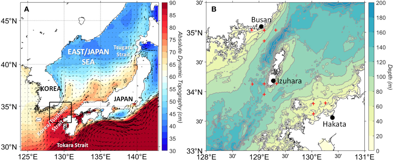
Figure 1 (A) Map showing the location of the Korea/Tsushima Strait (KTS) and climatological absolute dynamic topography (color) with geostrophic surface flow (vector) based on satellite altimetry from 1993 to 2017. (B) Tidal stations (black circles) at Busan, Izuhara and Hakata and the gridded altimetry data (red crosses, three or four nearest points at each tidal station) to calculate sea level differences across the straits. Colored contour lines show the bathymetry in meters.

Previous studies have reported that wind patterns over the North Pacific including the Okhotsk Sea can drive the annual mean and seasonal variability of volume transport through the KTS (Minato and Kimura, 1980; Ohshima, 1994; Tsujino et al., 2008; Ohshima and Kuga, 2023). In addition, large-scale atmosphere-ocean circulations, such as the Artic Oscillation, Asian winter monsoon, and Pacific Decadal Oscillation (PDO), have been suggested to control the transport variability on interannual to decadal time scales (Minobe et al., 2004; Gordon and Giulivi, 2004; Na et al., 2012). Moon and Lee (2016) reported a multi-decadal shift in the EJS sea level trend that shows a downward trend before the early 1980s, followed by an upward trend from the early 1980s onward. They suggested that the PDO-related wind stress curl may account for the trend shift in the EJS sea level during the 1980s, controlling the strength of the western boundary current in the subtropical gyre. This is also consistent with the previous observational study (Wang et al., 2016), confirming that the basin-wide wind stress curl may induce the weakening condition of Kuroshio in the ECS. Recently, Kida et al. (2021) found an increasing trend in the KTS transport from 1995 to 2018 based on sea level difference (SLD) data. Using numerical modeling result, they suggested that the increasing trend is forced by a northward shift in the Kuroshio axis south of Japan. These results may indicate trend shifts in the transport of subtropical warm water entering the EJS through the KTS. Because of the relatively short record of direct current measurements, however, the relationship between OHC changes in the EJS and long-term transport through the KTS has not been investigated, which is the main issue of this paper.

There have been few studies based on the observations of throughflow transport in the KTS. Previous estimates of annual transport in the KTS varied widely from 0.5 to 4.2 Sv (1Sv = 10⁶ m³ s⁻¹), depending on survey periods and methods (Toba et al., 1982; Isobe et al., 1994; Teague et al., 2002; Takikawa et al., 2005). Volume transport through the KTS has been measured using an acoustic Doppler current profiler (ADCP) on a ferryboat along the cruise line between Hakata in Japan and Busan in Korea since 1997. The estimated volume transport from the ferryboat ADCP for 1997−2007 was approximately 2.6 Sv, with seasonal variations in the range of 2–3.2 Sv (Fukudome et al., 2010). Although measurements volume transport through the KTS have been greatly improved by implementing the serial ferryboat ADCP in 1997, determining the long-term volume transport trend remains challenging because of relatively short measurement records. Because the throughflow in a strait is primarily in geostrophic balance (Figure 1A), sea level difference (SLD) across the strait has been used to estimate throughflow (Kawabe, 1982; Toba et al., 1982; Mizuno et al., 1989). A strong linear relationship between the KTS throughflow and the SLD across the strait was reported by Lyu and Kim (2003), who used cross-strait hydrographic sections to remove baroclinic effects. Takikawa and Yoon (2005) proposed an empirical formula relating volume transport to SLD using the first five years (1997–2001) of ferryboat ADCP current data. Based on their proposed formula, they estimated seasonality and long-term variation of volume transport with a roughly 15-year period. Recently, Lee (2016) and Shin et al. (2022) proposed a modified empirical formula that adopted the same approach of Takikawa and Yoon (2005) using the long-term ADCP data record from 1997 to 2013.

The present study is motivated by recently documented, but little investigated a relationship between the long-term transport through the KTS and upper-ocean warming in the EJS. Thus, this study aims at quantifying the long-term trend of throughflow transport in the KTS and investigating its connection with upper OHC in the EJS. To do so, we first utilize an updated formula for the relationship between throughflow and SLD across the KTS to estimate volume transport over the past four decades. We then use an ensemble empirical mode decomposition (EEMD) method to extract the nonlinear long-term trend from the estimated transport record in the KTS including many oscillating modes. Lastly, we discuss a connection between the trend in the TWC and the upper-ocean warming in the EJS.

2 Data and method

2.1 Data

SLD across the KTS was examined using tide gauge records from coastal tidal stations over the past four decades (1975–2017). Here, we used SLD values between Busan and Izuhara across the western channel and between Hakata and Izuhara across the eastern channel (blue circles in Figure 1B). Sea level data observed at Busan were obtained from the Korea Hydrographic and Oceanographic Agency and other tide gauge data were provided by the Japan Oceanographic Data Center. A 25-h low-pass filter was applied to remove tidal signals in the sea level records. An inverse barometric effect was removed using the atmospheric surface pressure from National Centers for Environmental Prediction (NCEP) reanalysis near the tidal stations, and we then used the monthly mean data to calculate SLD across the straits. Altimetry-based sea level observations dating back to 1993 from the AVISO dataset and volume transport measured by ferry-mounted ADCP operated by Research Institute for Applied Mechanics of Kyushu University [data from Fukudome et al. (2010)] since 1997 were also used to compare geostrophic transport estimated from SLD between the tide stations. The altimetry-based sea levels were averaged over the four nearest points to each tidal station to calculate SLD values across the straits (red crosses in Figure 1B).

To calculate OHC in the EJS, we used quality-controlled in situ profiles of Ishii and Kimoto (Ishii and Kimoto, 2009, hereafter, IK2009), which has been produced by objective analysis of measurements. This product consists of monthly gridded temperature and salinity with 1° spatial resolution and 16-depth levels from the surface to 700 m depth. In situ-based temperature data from the Met Office Hadley Centre (EN4, Good et al., 2013) was also used to compare the EJS OHC with the IK2009 product. EN4 dataset also provides monthly temperature and salinity with a spatial resolution of 1°. The OHC has been computed at each grid point of temperature by integrating down to 300 m from 1960 to 2009.

$\begin{array}{ll}OHC=\rho C_p{\displaystyle \iiint \theta dxdydz}& (1)\end{array}$

where $C_p$ is the specific heat capacity of seawater, $\rho$ is the water density, and $\theta$ is potential temperature. $x$, $y$, and $z$ are zonal, meridional, and vertical coordinates. In addition to in situ profile datasets, two different surface wind products were used to identify the relationship between the KTS throughflow and the large-scale wind patterns in the North Pacific: the 2.5° National Centers for Environmental Prediction/National Center for Atmospheric Research Reanalysis product from 1965 to 2010 (NCEP/NCAR), and the 1° European Center for Medium-Range Weather Forecasts ERA-Interim product from 1979 to 2010 (Dee et al., 2011).

2.2 Method

To estimate long-term geostrophic volume transport in the KTS, we utilized an empirical formula relating volume transport and SLD across the straits proposed by Takikawa and Yoon (2005). The empirical formula of geostrophic volume transport (VT) is given by:

$\begin{array}{ll}\text{VT}(t, \text{Δ}\eta )=\alpha (t)·v(\text{Δ}\eta )·S& (2)\end{array}$

where the unit of time t is month, $\text{Δ}\eta$ is SLD across the straits, and S is the strait’s cross-sectional area (11.61 km² for the eastern channel and 6.66 km² for the western channel). $v(\text{Δ}\eta )$ is the geostrophic velocity for the relation between the surface current velocity (v) and SLD across the straits. Takikawa et al. (2005) have shown strong seasonal variations in current baroclinicity and volume transport in the KTS by analyzing ADCP measurements from 1997 to 2001. To incorporate the effect of current baroclinicity in the transport estimation from SLD, Takikawa and Yoon (2005) calculated the monthly regression lines between the volume transport estimated from the ADCP data and the SLD using tide gauge data. Then, the monthly gradients of the regression lines were fitted by a function [$\alpha (t)$] with annual and semi-annual periods using the least squares method (Takikawa and Yoon, 2005).

$\begin{array}{ll}\alpha (t)={\alpha }_0+a_{1}cos\frac{\pi }{6}t+b_{1}sin\frac{\pi }{6}t+a_{2}cos\frac{\pi }{3}t+b_{2}sin\frac{\pi }{3}t& (3)\end{array}$

where the unit of time t is month, and ${\alpha }_0, a_1,a_2,b_1$, and $b_2$ indicate the regression coefficients using the least square method. This function incorporates the effect of current baroclinicity and seasonality on volume transport estimation from the SLD using tide gauge records. Recently, Lee (2016) and Shin et al. (2022) modified the regression coefficients of the function (Eq. 2) using the extended ADCP data from 1997 to 2013.They also applied the same method above (Takikawa and Yoon, 2005) using altimetry absolute dynamic topography (ADT) data for the 1997–2013 period and obtained the monthly gradient of the regression lines between the transport calculated from the ADCP data and the geostrophic relation using the ADT data. The regression coefficients for tide gauge and altimetry data modified by Lee (2016) are listed in Table 1. The detailed descriptions of the computation process can be found in Takikawa and Yoon (2005). In this study, we used the updated regression coefficients to estimate long-term volume transport using SLD between the two tide gauge stations over the past four decades. To validate the consistency of the empirical formula, we also compared the volume transport estimated from the tide gauge data with that estimated from the altimeter data.

TABLE 1

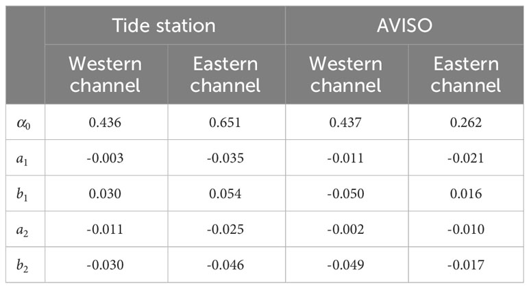
Table 1 Regression coefficients of the function Eq. (3) for tide station and altimetry data [from Lee (2016)].

Volume transport estimated using long-term SLD was decomposed into variability of different time scales and a nonlinear trend using the EEMD method. The EEMD method is based on empirical mode decomposition (EMD), which is designed to separate the time series into a finite number of intrinsic model functions (IMFs) and a residual that represents the long-term adaptive trend (Huang et al., 1998). The final IMF in the EEMD process is obtained as an ensemble average of corresponding IMFs that was decomposed from the targeted time series data with white noise added by the EMD (Huang and Wu, 2008). The total number of IMFs is determined automatically in the EMD process and depends on the length of the original signal. Unlike the traditionally used filtering or curve-fitting methods based on assumptions of stationarity and linearity, the intrinsic trend requires no predetermined functional form and can vary with time. The benefit of using EEMD is that it can separate a time-varying trend from non-stationary oscillations such as natural variability on different time scales. Because sea-level data are nonstationary and nonlinear natural processes, which are not completely known, it is appropriate to analyze and deal with nonstationary datasets using EEMD method based on data only. For this reason, EEMD has been widely used in various signal analysis fields including climate research (e.g., Lee, 2013; Jo et al., 2014; Chen et al., 2017; Cha et al., 2018). In this paper, we used the EEMD method to extract a nonlinear trend from the geostrophic volume transport estimated from SLD across the KTS, without any prior assumption about the shape of a trend. To determine whether the obtained IMFs contain useful information, statistical significance tests are performed, comparing spectral energy of each decomposed mode with that of white noise. This method, based on the characteristics of Gaussian white noise with EMD, was proposed by Wu and Huang (2004), who showed improved IMF statistical significance through a rescaling step using noise. This method works as follows: 1) decompose the targeted noisy dataset into IMFs, 2) calculate the spread function of various percentiles for the white noise and select the confidence limit level, and 3) compare energy densities for the IMFs from noisy data with the spread functions. In this test, we calculated the spread function of the 99% and 95% confidence limit levels and determined the spread lines for the confidence level, which bound the energy of white noise with upper and lower limits. If the calculated energy density of any IMF lies below the these spread lines, then the IMF is not distinguishable from the white noise, i.e., the IMF contains no information. If the energy level of any IMF lies above the spread lines, then we can assume that it contains statistically significant information. Interested readers are referred to Wu and Huang (2004) for more details on the process of significance test and its physical meanings.

In addition, a bootstrap method, which is based on random resampling to estimate confidence intervals, is used to test the significance of the intrinsic trends obtained from EEMD. The main steps of this method are as follows (Park et al., 2018): 1) artificial resampled data (${\epsilon }_{rand}$) are created by randomly sampling the anomaly for the original data. 2) the artificial data and the residual (R) derived from the EEMD are then added ($x^{*}={\epsilon }_{rand}+R$), 3) the EEMD is again performed on the reconstructed data ($x^{*}$), after which the artificial trend can be obtained, and 4) steps 1–3 are repeated M times (in this study, M = 1,000 iterations). The mean artificial trend can then be estimated from the individual bootstrap simulations ($R(x_i^{*}$): $\overline{R^{*}}=\frac{1}{m}{\displaystyle {\sum }_{i=1}^{M}R(x_i^{*})}$). Confidence intervals can be calculated from all the artificial trends using a standard Student’s t-test distribution.

3 Geostrophic volume transport estimated from SLD

Using Eq. (2), we estimated the monthly mean geostrophic volume transport through the KTS from SLD using tide gauge data between Busan and Izuhara (western channel) and between Hakata and Izuhara (eastern channel) from 1975 to 2017 (Figure 2). To examine the validity of the geostrophic transport, we compared it with ship-mounted ADCP-measured volume transport from 1997 to 2012 (blue lines in Figure 2). The estimated total volume transports showed very good agreement with those ADCP-measured values, with statistically significant correlation coefficients exceeding 0.85 and a root-mean-square error (RMSE) of less than 0.24 Sv. The correlation coefficient and RMSE in the western channel were 0.89 and 0.16 Sv, respectively, which shows relatively good correlation compared with that in the eastern channel. In addition to ADCP measurements, the sea level anomalies (SLA) measured by satellite altimetry were also used for the comparison (red lines in Figure 2). The volume transport estimated from SLD derived from tide gauge data again matched well with the altimetry-based SLA estimate.

FIGURE 2

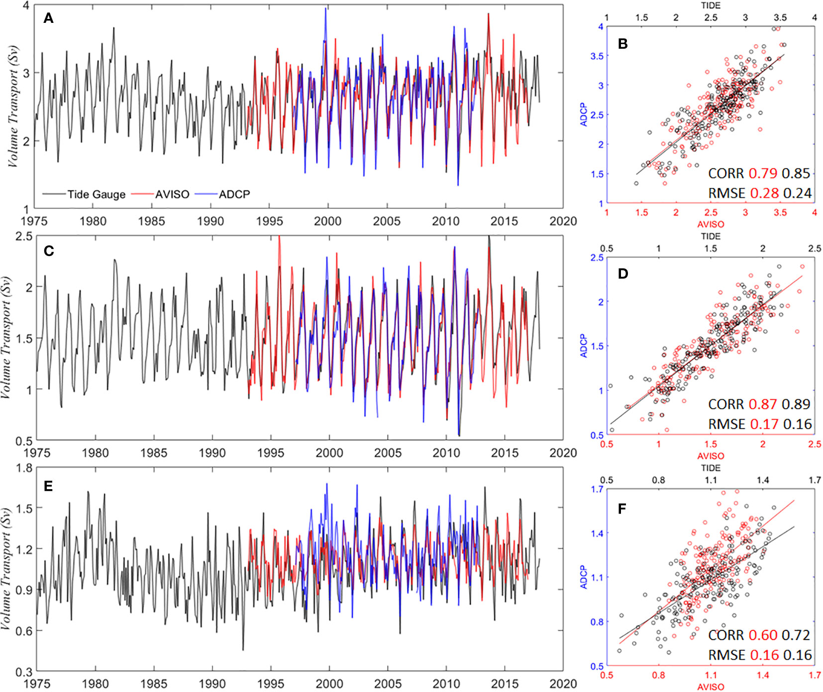
Figure 2 (Left panels) Monthly volume transport (Sv, 1Sv = 10⁶ m³ s^–1) of the Tsushima Warm Current from 1975 to 2017 estimated from sea level differences (SLD) using Eq. (1) (black lines): (A) the Korea/Tsushima Strait (KTS), (C) the western channel and (E) the eastern channel. Blue and red lines indicate the monthly volume transports measured by ferry-mounted ADCP for 1997–2012 and estimated from altimetry-based sea level anomalies (SLA) for 1993–2017, respectively. Comparison of SLD-estimated volume transports with altimetry-based SLA (red) and the ferry-mounted ADCP (blue) volume transport: (B) the KTS, (D) the western channel, and (F) the eastern channel. SLD-estimated transport is shown by black dots in (B, D, F).

The estimated volume transport through the KTS averaged over 43 years was 2.61 Sv, with 1.51 Sv through the western channel and 1.05 Sv through the eastern channel. These values are almost identical to previous estimates (Takikawa et al., 2005; Fukudome et al., 2010). The long-term geostrophic transport includes internal variability on intraseasonal to decadal time scales, with a dominant seasonal cycle mode. Seasonally varying transport in the KTS has a wintertime minimum and two significant maxima in spring and autumn in most years. Additionally, there is a larger seasonal amplitude in the western channel than in the eastern channel (Figures 2C, E). The seasonality features in the KTS have been well documented in previous works; however, few studies have examined the long-term trends that are potentially affected by intraseasonal to decadal variability.

4 Long-term trend of volume transport in the KTS

To extract an intrinsic trend from the SLD-estimated geostrophic volume transport, we conducted an EEMD analysis for transport through the KTS (i.e., western and eastern channels as well as the KTS as a whole). This yielded eight IMFs and a residual based on their timescales (Figure 3). We also performed a significance test on the EEMD-derived IMFs by comparing the spectral energy of each decomposed mode with that of white noise to determine whether the individual IMFs contained statistically significant information. The test result indicated that all IMFs except for IMF 8 for the estimated volume transports, were significant compared to white noise at the 95% confidence limit level (Figure 4). This means that all IMFs can be distinguishable from Gaussian white noise at the 95% confidence level. The frequency of EEMD-derived signals was estimated by Hibert spectral analysis. Spectral analysis indicated that the first two IMFs showed high-frequency components at less than one year, and IMF3 to IMF5 cover interannual scale frequencies varying from 1.5 to 6.6 years. Among the IMFs, IMF2 has the highest energy density, with mean period of 1 year. The corresponding periods of IMF6 and IMF7 were 11 years and 16.5 years, respectively. This shows that the low-frequency modes were separated well from the original signal. Takikawa and Yoon (2005) also reported a decadal variation of roughly 15 years, which is a similar period to that of the IMF6 and IMF7 obtained from the SLD-estimated volume transport. Following the definition of the EEMD method, the intrinsic trend is distinguishable from all IMFs, which implies that the internal modes do not contribute to the intrinsic trend over the whole period.

FIGURE 3

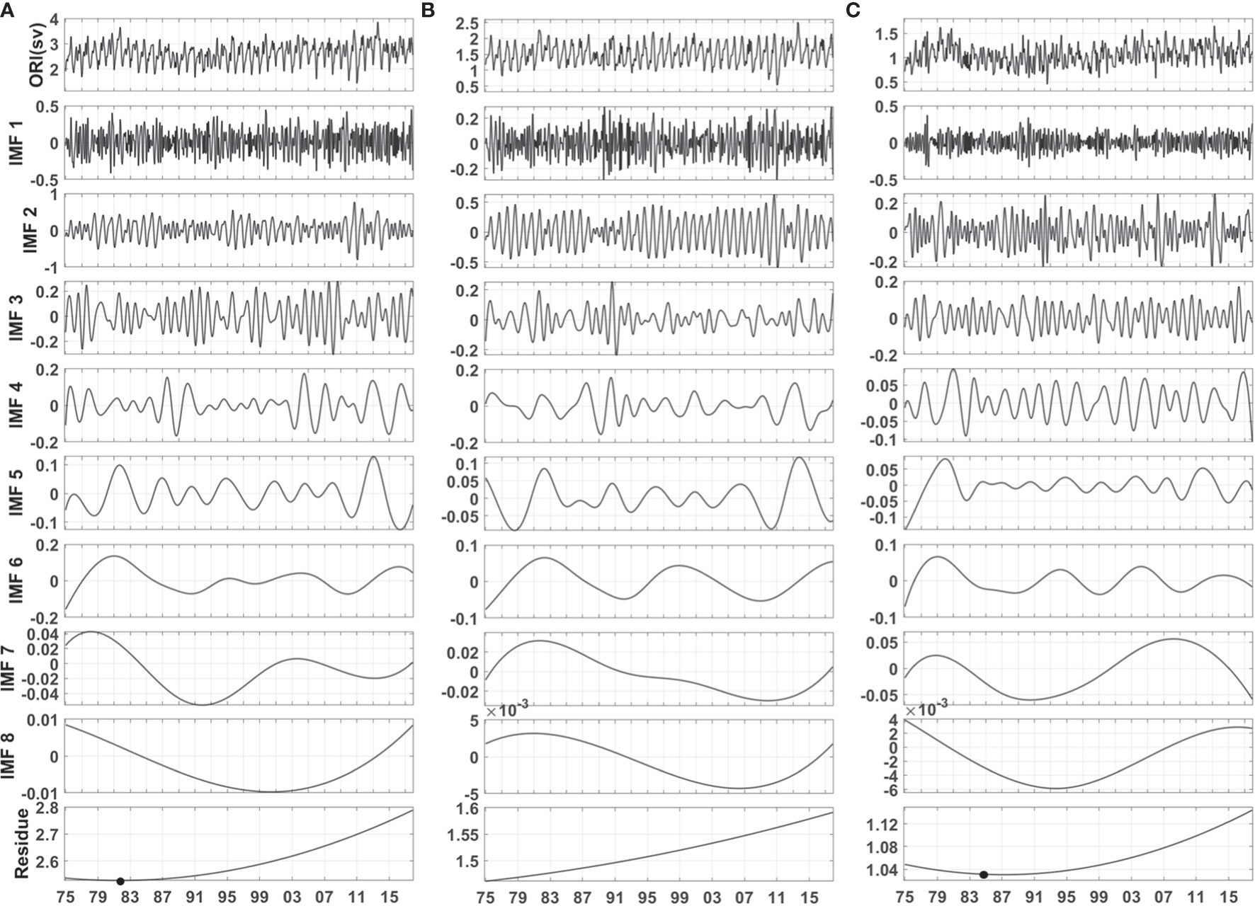
Figure 3 EEMD decompositions of monthly volume transports through (A) the Korea/Tsushima Strait, (B) the western channel and (C) the eastern channel estimated from sea level differences across the straits. Original monthly data (top) are decomposed into eight IMFs from high to low frequency and resulting trends (bottom panels) by EEMD analysis. Black circles indicate the shifting years of the EEMD-derived trend.

FIGURE 4

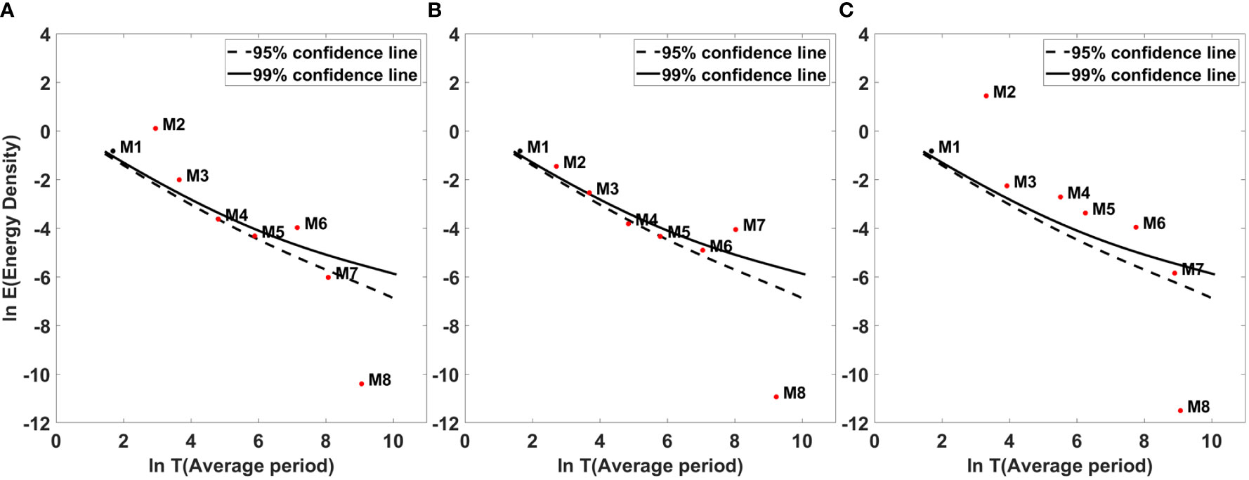
Figure 4 Statistical significance tests of all IMFs of the monthly volume transports through (A) the Korea/Tsushima Strait, (B) the western channel and (C) the eastern channel estimated from sea level differences across the straits. The solid and dashed lines represent the 99% and 95% confidence levels, respectively.

The intrinsic trends (i.e., residual mode) and the instantaneous rates of volume transport in the KTS are shown in Figures 5, 6, respectively. The significance of the intrinsic trend was tested using a bootstrap method (Mudelsee, 2010; Ezer and Corlett, 2012; Park et al., 2018) that is based on random resampling to estimate confidence intervals. As shown in Figure 5, although the artificial mean (i.e., ensemble of bootstrap simulations) trend (dashed lines) slightly differs from the original trends (solid lines), the time-varying trends do not change significantly within the confidence intervals. This indicates the trends derived from EEMD analysis are robust. Volume transport through the KTS exhibited a nonlinear trend with a decreasing or near-stationary trend prior to the mid-1980s and an increasing trend after that (Figure 5A). The instantaneous rate, which indicates the rate of the time-varying trend by calculating the temporal derivative of the trend, was approximately -0.01 Sv per decade in 1975 and increased to 0.08 Sv per decade in 2017 (Figure 6A). Although the transport trend slowly increased over four decades, its shift around the 1980s was robust. The time-varying nature of the transport trend suggests an acceleration in volume transport through the KTS, with the persistent increase in the trend rate occurring after the mid-1980s. Of particular interest is that the shift in the trend in the mid-1980s mainly arose from volume transport changes in the eastern channel rather than in the western channel (Figures 5B, C). Volume transport through the western channel showed a slightly increasing trend over the whole period, going from 1.45 Sv at the beginning to 1.6 Sv at the end. The rate of the transport trend in the western channel was much smaller than that in the KTS overall, corresponding to only about 20% of the trend rate in the KTS. Unlike the western channel, volume transport through the eastern channel showed a decreasing trend prior to around 1984 and an increasing trend after that (Figures 5C, 6C). In other words, a change in the trend is occurred in the mid-1980s. The rate increased by 0.07 Sv per decade, going from approximately –0.02 Sv per decade in 1975 to around 0.05 Sv per decade in 2017, exhibiting an acceleration of the trend in agreement with that in the KTS as a whole (Figure 6C). The EEMD-derived trend in the KTS is characterized by a shift in the long-term trend from a decreasing trend to an increasing one during the mid-1980s, which emphasizes that the trend reversal is the dominant change in the volume transport over the past 40 years. It should be noted that the potential multi-decadal variability of the volume transport through the KTS on timescales longer than that of the collected data cannot be separated from the intrinsic trend. This means that the shifted trend of the volume transport may partially reflect internal variability on multi-decadal time scales.

FIGURE 5

Figure 5 Time-varying trends from EEMD analysis of volume transport (Sv, 1Sv = 10⁶ m³ s^–1) estimated from sea level differences with bootstrap simulations (M = 1000 iterations) for the significance test: (A) the Korea/Tsushima Strait, (B) the western channel and (C) the eastern channel. The thin gray lines indicate all simulated individual trends. The solid and dashed lines are the trends of the original data mean and artificial mean, respectively. The 90% confidence intervals are shown by the shaded areas.

FIGURE 6

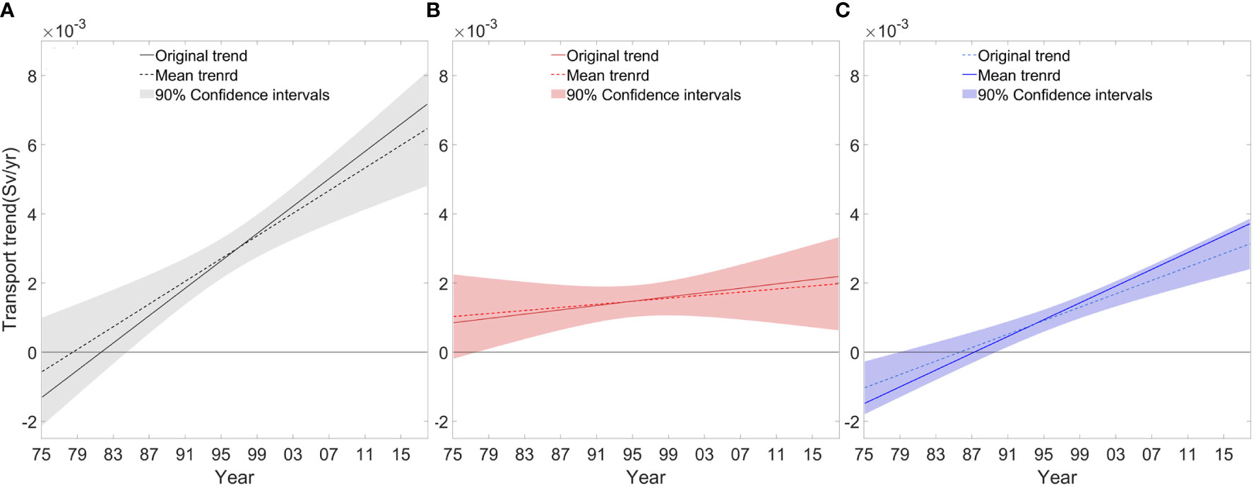
Figure 6 The instantaneous rate (Sv year^–1) of the trends from EEMD analysis of volume transport estimated from the sea level differences with bootstrap simulations (M = 1000 iterations) for the significance test: (A) the Korea/Tsushima Strait, (B) the western channel and (C) the eastern channel. The solid and dashed lines are the trend rates of the original mean and artificial mean, respectively. The 90% confidence intervals are shown by the shaded areas.

5 Upper-ocean warming in the East/Japan Sea

As suggested in previous studies, the warm and salty TWC flowing through the KTS affects upper-ocean circulation and sea level rises in the EJS, which correspond to thermal expansion associated with oceanic warming. Figure 7A shows the time series of the basin mean of yearly OHC anomaly (relative to the long-term mean) in the uppermost 300 m of the EJS from 1960 to 2010 based on the in situ profiles of IK2009 and EN4 reanalysis. The variability in the two time series agree quite well each other over the entire period of 1960–2010, with correlation coefficient of 0.89, and no discernible difference in trend. This striking agreement between the two products of temperature enhances confidence in the estimated OHC variability. The time series was characterized by a long-term shift in the OHC trend, which was superimposed on a dominant decadal fluctuation. The mean OHC over the EJS revealed a declining trend prior to the mid-1980s, followed by an increasing trend after that. This is consistent with the long-term trend shift in SLD-estimated volume transport through the KTS, particularly in the eastern channel. The EEMD-derived intrinsic trend of mean OHC also detected the reversed trend since mid-1980s (Figure 7B). The EEMD analysis was conducted using the monthly gridded OHCs and yielded total eight IMFs and a residual. The bootstrap method was also used to test the significance of the intrinsic trend obtained from EEMD. The extracted OHC trend is within the confidence interval, indicating the robustness of the EEMD-derived trend. The OHC in the EJS showed a nonlinear trend with a decline trend prior to around 1984 and an upward trend after that, emphasizing that the trend reversal is the dominant change in the upper-ocean OHC in the EJS over the past decades. The shifting year in the OHC trend matches well with the change of transport trend in the eastern channel, showing no significant time lags. Furthermore, the reversed trend was more clearly identified in Figure 8, which shows the spatial patterns of the OHC trend in the uppermost 300 m depth derived from IK2009 and EN4 over the periods of 1960–1985 and 1986–2010, respectively. Prior to mid-1980s, negative OHC trends prevailed over the southeastern parts of the EJS, extending northeast to southwest east of 135°E along the west coast of Japan, whereas there was a positive trend in the western EJS along the east coast of Korean Peninsula. The trend of upper-OHC trend in the southeastern EJS was fully reversed from the mid-1980s onward, except for the western EJS along the Korean Peninsula. This indicates that significant warming in the EJS, particularly in the southeastern part, has been persistent over the past few decades, which represents a long-term trend shift beginning in the mid-1980s. In contrast, there was a persistent warming trend in the western EJS along the Korean Peninsula, which may be connected with the increasing trend of volume transport through the western channel over the whole period.

FIGURE 7

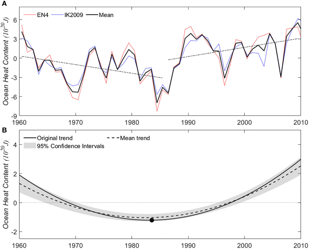
Figure 7 (A) Time series of upper 300 m ocean heat content (OHC) anomaly in the East/Japan Sea (EJS) derived from in situ-based IK2009 (blue) and EN4 (red line) datasets from 1960 to 2010. The linear trend lines for 1960–1985 and 1986–2010 are also presented (dashed lines). (B) Time-varying trend from EEMD analysis of EJS OHC. Solid and dashed lines are the trend of original data mean and artificial mean, respectively. The 95% confidence intervals are shown by the shaded areas. Black circle indicates the shifting year of the EEMD-derived original trend.

FIGURE 8

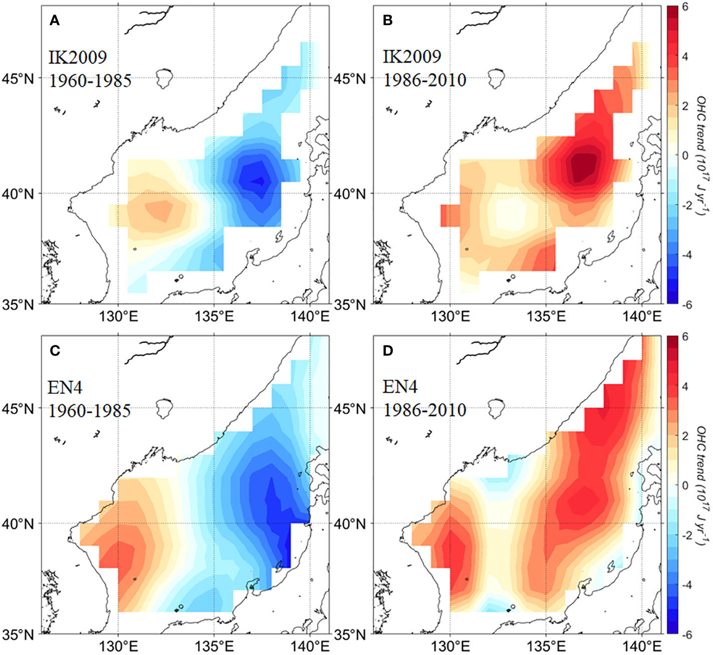
Figure 8 Spatial trends of OHC in the uppermost 300 m depth of the EJS derived from IK2009 (upper) and EN4 (lower panels) datasets over two periods: (A, C) 1960–1985 and (B, D) 1986–2010.

It has been proposed that the OHC in the EJS is associated with upper-ocean circulation because of the variability of the TWC through the KTS (Isobe and Isoda, 1997; Yoon and Kim, 2009). Na et al. (2012) suggested a linkage between decadal OHC variability in the EJS superimposed on an upward trend and variability in the northwestern Pacific via variability of the TWC through the KTS. Our results indicate that the warming signal in the EJS is closely linked to the trend shift of the TWC through the KTS. A similar shift in the trend was recently reported by Moon and Lee (2016), who showed that the EJS underwent a significant increasing trend in sea levels from the mid-1980s to 2008 due to a strengthening trend of positive wind stress curl at mid-latitudes in the western and central North Pacific that was negatively correlated with the PDO (Andres et al., 2009). Following the above discussions, the time-varying trend of volume transport through the KTS we estimated is likely a key component of upper-ocean warming in the EJS in recent decades, reflecting a connection between OHC in the EJS and the TWC through the KTS.

6 Trend shifts in the throughflow and large-scale winds

Large-scale wind-driven circulations in the North Pacific have been suggested as the driving mechanism of inflow through the KTS (Minato and Kimura, 1980; Ohshima, 1994; Nof, 2000). Minato and Kimura (1980) reported that the SLD between the two straits (i.e., the KTS and the Tsugaru strait) connecting a marginal sea to an open ocean, which is induced by wind-driven gyres, can drive the inflow and outflow through the straits. This idea was applied to a numerical model with a realistic topography by Ohshima (1994) who successfully estimated the throughflow transports in the straits. Lyu and Kim (2005) also extended the idea on the timescales from sub-inertial to interannual using a simple analytical model. Thus, the wind-driven circulations can be one of the important factors for regional SLD and its long-term trend that dynamically drives the inflow of an open ocean water into a marginal sea.

To identify a connection between the trend shift in the KTS transport and large-scale wind patterns in the North Pacific, we examined the long-term trends of wind stress curl (WSC, $\nabla \times \overrightarrow{\tau }$) derived from NCEP reanalysis over the following two periods: 1965−1985 and 1986−2010 (Figure 9). Before the mid-1980s, the trend of basin-wide WSC in the subtropical region tended to be negative, but it tended to be positive in the subpolar region (Figure 9A). On the other hand, the WSC trends were reversed after the mid-1980s, i.e., a positive trend in the subtropical and a negative trend in the subpolar regions (Figure 9B). These changes of WSC are associated with the PDO pattern that corresponds to counter-rotating wind patterns at mid- and high-latitudes in the western/central North Pacific. Based on the regression and correlation analysis, Moon and Lee (2016) showed an imprint of PDO on the surface wind patterns in the subtropical and subpolar regions of the North Pacific. The trends of the two WSC bands were clearly evident in the time series of regionally averaged WSC and EEMD-determined trends at the two bands (Figures 9C, D). We conducted the EEMD analysis using the monthly wind datasets and obtained total eight IMFs and a residual. The nonlinear trend in the WSC at mid-latitudes has a shifting point around 1984, which is consistent with the timing of the shifting trend in the EJS OHC. This indicates that the PDO-related large-scale WSC shift matches with the trend shifts in the KTS throughflow and the EJS OHC. It should be noted that as the PDO varied on interannual timescales from late 1990s, the long-term curl trend from that time may be related to other causes like climate change.

FIGURE 9

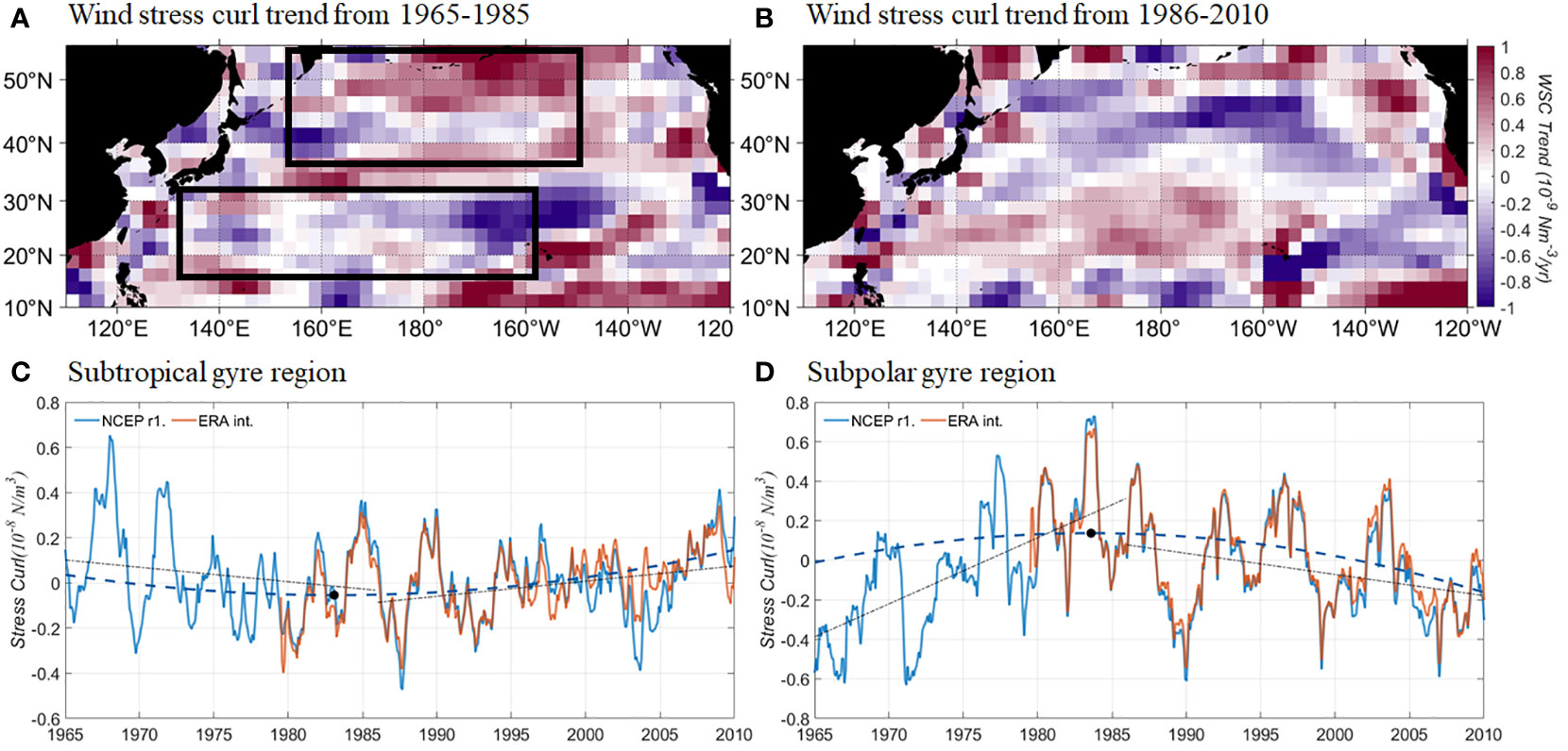
Figure 9 (A, B) Trends of wind stress curl derived from NCEP reanalysis product over multi-decadal period, i.e., 1965-1985 and 1986-2010. Time series of mean wind stress curls anomalies over the North Pacific at (C) mid-latitudes [subtropical gyre region shown by southern box in (A)] and (D) high-latitudes [subpolar gyre region shown by northern box in (A)] from the reanalysis products of NCEP (blue) and ERA interim (red). The multi-decadal linear trends (thin lines) and EEMD-derived trends (dashed lines) are also presented. Black circles indicate the shifting points of the EEMD-derived trends.

Prior to the mid-1980s, the PDO-related negative trend of the WSC at mid-latitudes can force stronger Sverdrup flow in the subtropical gyre, which is compensated for by a stronger return Kuroshio in the ECS (Andres et al., 2009; Moon and Lee, 2016). The enhanced Kuroshio flow due to the negative WSC trend may result in a low sea level in the northern shelf of the ECS, which lies at the entrance of the KTS, because the Kuroshio jet is intertially controlled to continue in a straight path through the Tokara strait (Andres et al., 2009; Moon and Song, 2017). This relation was also reported by Moon and Song (2017) who have shown a sea level fall in the ECS during this period, using a global ocean circulation model. On the other hand, these relations were reversed during the period since the mid-1980s when the PDO index shifted toward an opposite pattern that of the previous decades. The weakened negative WSC in the subtropical region from the mid-1980s to the present forced a weaker Sverdrup flow including the Kuroshio jet in the ECS. When the ECS-Kuroshio jet along the 200 m-isobaths of the shelf slope is weak due to a positive trend of WSC in the mid-latitude after mid-1980s, it is steered to the north of topography southwest of Kyushu, Japan and warmer water enters the EJS through the KTS, particularly in the eastern channel. This connection was also reported by a recent study of Shin et al. (2022) who have shown that the transport through the KTS is inversely correlated with the Kuroshio transport to the south of Japan and the PDO index. The recent increasing trend in the eastern channel is also consistent with the result of Kida et al. (2021), which found a relationship between the throughflow in the eastern channel and the Kuroshio axis over 1995–2018. They argued that a northward shift in the Kuroshio and Kuroshio extension axes brings the subtropical gyre with sea level rise along the south coast of Japan, which propagates toward the eastern channel of KTS along the coast, resulting in enhancement of KTS throughflow transport. These results suggest that the contrasting WSC trends over the North Pacific may be a key driver in determining the trend shifts in the inflow through the KTS and the upper-ocean warming in the EJS over the past decades. Nevertheless, because the data analysis alone may have limitations in delineating the underlying physics clearly, further studies based on numerical modeling are needed to clarify the relationship between the KTS throughflow and the climate-driven upper-ocean circulations.

7 Summary

This study aimed at quantifying the long-term trend of throughflow transport in the KTS and investigating its connection with the recent warming trend in the EJS. Based on the geostrophic relation between throughflow and SLD across the KTS, we estimated long-term volume transport using tide gauge data from the past four decades. The estimated geostrophic transport matched well with ship-mounted ADCP measurements and estimates from the altimetry-based SLA, which corroborates the reliability of estimated long-term volume transport. Then, we used an EEMD method on the estimated transport time series to separate an intrinsic trend from non-stationary oscillations on different time scales. The throughflow in the KTS exhibited a nonlinear trend that was decreasing or near-stationary prior to the mid-1980s and increasing after that. The EEMD analysis revealed an acceleration in volume transport, with a persistent increase in the trend rate after the mid-1980s. The shift during the mid-1980s mainly arose from volume transport changes in the eastern channel rather than in the western channel.

Further analyses of upper OHC in the EJS showed that the trend shift in the KTS closely coincided with an upper-ocean warming trend in the EJS after the mid-1980s. These results supported the role of the TWC in upper-ocean circulation in the EJS suggested by previous studies (e.g., Gordon et al., 2002; Na et al., 2012; Moon and Lee, 2016), which represents a linkage between the warming signal in the EJS and the trend shift of the TWC through the KTS. Analyzing the WSC patterns showed that the long-term shift in the KTS throughflow may be closely associated with the large-sale wind-driven circulations in the North Pacific. Prior to the mid-1980s, the trend of basin-wide WSC in the subtropical region tended to be negative that can result in a low sea level in the northern ECS, whereas it tended to be positive in the subpolar region that can result in a high sea level outside the Tsugaru strait. It is therefore expected that the SLD between the entrance of the KTS and the outside the Tsugaru strait became small, and consequently the transport of warm subtropical water entering the EJS through the KTS became weak, thereby decreasing the upper-ocean warming and sea level in the EJS. On the other hand, these wind-driven responses of the KTS throughflow were reversed after the mid-1980s when the WSC trends in the North Pacific were shifted toward an opposite pattern that of the previous decades. These results suggest that the contrasting WSC trends over the North Pacific may be a key driver in determining the trend shifts in the inflow through the KTS and the upper-ocean warming in the EJS over the past four decades. Nevertheless, unlike the transport trend through the eastern channel, there was no trend shift with a slightly accelerating rate in the western channel, suggesting that the warming trend in the EJS is unlikely to be a simple process, but is rather likely to be a complex process involving the regional upper-ocean circulation (e.g., the water from the Taiwan Current and the Yellow Sea) and atmospheric forcing. Although not pursued in this study, the TWC’s effect on upper OHC in the EJS must be investigated in future studies to clarify the dynamic linkage between them.

This study has also implications for predictions of regional climate conditions. For example, Hirose et al. (2009) noted that volume transport through the KTS largely drives precipitation over the Japanese Islands via ocean-to-atmosphere feedback. Therefore, the estimated long-term volume transport of the TWC could be useful for better understanding of the regional climate system associated with upper-ocean warming in the EJS.

Data availability statement

Publicly available datasets were analyzed in this study. This data can be found here: https://www.aviso.altimetry.fr/en/data/products/sea-surface-height-products/global/gridded-sea-level-heights-and-derived-variables.htm; https://www.esrl.noaa.gov/psd/data/gridded/data.ncep.reanalysis.html; http://www.metoffice.gov.uk/hadobs/en4/download-en4-2-0.html.

Author contributions

J-HM and TK contributed to the conception and design of the study. HJ and HC contributed to the data processing and analysis. NH contributed to scientific discussion. The paper was written by J-HM with input from all authors. All authors contributed to the article and approved the submitted version.

Funding

The author(s) declare financial support was received for the research, authorship, and/or publication of this article. This research was supported by the National Research Foundation of Korea (NRF) grant funded by the Korea government (MIST) (NRF-2022M3I6A1086449) and Korea Institute of Marine Science & Technology (KIMST) funded by the Ministry of Oceans and Fisheries (RS-2023-00256330, Development of risk managing technology tackling ocean and fisheries crisis around Korean Peninsula by Kuroshio Current). TK was supported by the National Research Foundation of Korea (NRF) grant funded by the Korea government (MSIT) (NRF-2023R1A2C1006812).

Conflict of interest

The authors declare that the research was conducted in the absence of any commercial or financial relationships that could be construed as a potential conflict of interest.

Publisher’s note

All claims expressed in this article are solely those of the authors and do not necessarily represent those of their affiliated organizations, or those of the publisher, the editors and the reviewers. Any product that may be evaluated in this article, or claim that may be made by its manufacturer, is not guaranteed or endorsed by the publisher.

References

Andres M., Park J. H., Wimbush M., Zhu X. H., Nakamura H., Kim K., et al. (2009). Mainfestation of the pacific decadal oscillation in the Kuroshio. Geophys. Res. Lett. 36, L16602. doi: 10.1029/2009GL039216

CrossRef Full Text | Google Scholar

Cha S.-C., Moon J.-H., Song Y. T. (2018). A recent shift toward an El Niño-like ocean state in the tropical pacific and the resumption of ocean warming. Geophys. Res. Lett. 45, 11,885–11,894. doi: 10.1029/2018GL080651

CrossRef Full Text | Google Scholar

Chang K.-I., Teague W. J., Lyu S. J., Perkins H. T., Lee D-K., Watts D. R., et al. (2004). Circulation and currents in the southwestern East/Japan Sea: Overview and review. Prog. Oceanogr. 61, 105–156. doi: 10.1016/j.pocean.2004.06.005

CrossRef Full Text | Google Scholar

Chen X., Zhang X., Church J. A., Watson C. S., King M. A., Monselesan D., et al. (2017). The increasing rate of global mean sea-level rise during 1993–2014. Nat. Clim. Change. 7, 492–495. doi: 10.1038/nclimate3325

CrossRef Full Text | Google Scholar

Dee D. P., Uppala S. M., Simmons A. J., Berrisford P., Poli P., Kobayashi S., et al. (2011). The ERA-Interim reanalysis: Configuration and performance of the data assimilation system. Q. J. R. Meteorol. Soc 137,656 553–597. doi: 10.1002/qj.828

CrossRef Full Text | Google Scholar

Ezer T., Corlett W. B. (2012). Is sea level rise accelerating in the Chesapeake Bay? A demonstration of a novel new approach for analyzing sea level data. Geophys. Res. Lett. 39, L19605. doi: 10.1029/2012GL053435

CrossRef Full Text | Google Scholar

Fukudome K.-I., Yoon J.-H., Ostrovskii A., Takikawa T., Han I.-S. (2010). Seasonal volume transport variation in the tsushima warm current through the tsushima straits from 10 years of ADCP observations. J. Oceanogr. 66, 539–551. doi: 10.1007/s10872-010-0045-5

CrossRef Full Text | Google Scholar

Good S. A., Martin M. J., Rayner N. A. (2013). EN4: Quality controlled ocean temperature and salinity profiles and monthly objective analyses with uncertainty estimates. J. Geophys. Res.: Oceans. 118, 6704–6716. doi: 10.1002/2013JC009067

CrossRef Full Text | Google Scholar

Gordon A. L., Giulivi C. F. (2004). Pacific decadal oscillation and sea level in the Japan/East sea. Deep-Sea Res. I. 51, 653–663. doi: 10.1016/j.dsr.2004.02.005

CrossRef Full Text | Google Scholar

Gordon A. L., Guilivi C. F., Lee C. M., Furey H. H., Bower A., Talley L. (2002). Japan/East Sea intrathermocline eddies. J. Phys. Oceanogr. 32, 1960–1974. doi: 10.1175/1520-0485(2002)032<1960:JESIE>2.0.CO;2

CrossRef Full Text | Google Scholar

Han I. S., Kang Y.-Q. (2003). Supply of heat by Tsushima warm current in the East Sea (Japan Sea). J. Oceanogr. 59, 317–323. doi: 10.1023/A:1025563810201

CrossRef Full Text | Google Scholar

Hirose N., Kim C.-H., Yoon J.-H. (1996). Heat budget in the Japan sea. J. Oceanogr. 52, 553–574. doi: 10.1007/BF02238321

CrossRef Full Text | Google Scholar

Hirose N., Nishimura K., Yamamoto M. (2009). Observational evidence of a warm ocean current preceding a winter teleconnection pattern in the northwestern Pacific. Geophys. Res. Lett. 36, L09705. doi: 10.1029/2009GL037448

CrossRef Full Text | Google Scholar

Huang N. E., Shen Z., Long S. R., Wu M. C., Shih H. H., Zheng Q., et al. (1998). The empirical mode decomposition and the Hilbert spectrum for nonlinear and non-stationary time series analysis. Proc. R. Soc A: Math. Phys. Eng. Sci. 454, 903–995. doi: 10.1098/rspa.1998.0193

CrossRef Full Text | Google Scholar

Huang N. E., Wu Z. (2008). A review on Hilbert-Huang transform: Method and its applications to geophysical studies. Rev. Geophys. 46, RG2006. doi: 10.1029/2007RG000228

CrossRef Full Text | Google Scholar

Ishii M., Kimoto M. (2009). Reevaluation of historical ocean heat content variations with time-varying XBT and MBT depth bias corrections. J. Oceanogr. 65, 287–299. doi: 10.1007/s10872-009-0027-7

CrossRef Full Text | Google Scholar

Isobe A., Isoda Y. (1997). Circulation in the Japan basin, the northern part of the Japan Sea. J. Oceanogr. 53, 373–381. doi: 10.1016/0278-4343(94)90003-5

CrossRef Full Text | Google Scholar

Isobe A., Tawara S., Kaneko A., Kawano M. (1994). Seasonal variability in the Tsushima warm current, Tsushima-Korea strait. Cont. Shelf Res. 14, 23–35. doi: 10.1016/0278-4343(94)90003-5

CrossRef Full Text | Google Scholar

Jo Y.-H., Breaker L. C., Tseng Y.-H., Yeh S.-W. (2014). A temporal multiscale analysis of the waters off the east coast of south Korea over the past four decades. Terr. Atmos. Ocean Sci. 25, 415–434. doi: 10.3319/TAO.2013.12.31.01(Oc)

CrossRef Full Text | Google Scholar

Kang S. K., Cherniawsky J. Y., Foreman M. G. G., Min H. S., Kim C.-H., Kang H.-W. (2005). Patterns of recent sea level rise in the East/Japan Sea from satellite altimetry and in situ data. J. Geophys. Res. 110, C07002. doi: 10.1029/2004JC002565

CrossRef Full Text | Google Scholar

Katoh O. (1994). Structure of the Tsushima current in the Southwestern Japan sea. J. Oceanogr. 52, 317–338. doi: 10.1007/BF02239520

CrossRef Full Text | Google Scholar

Kawabe M. (1982). Branching of the Tsushima Current in the Japan Sea part II. numerical experiment. J. Oceanogr. Soc Japan 38, 183–192. doi: 10.1007/BF02111101

CrossRef Full Text | Google Scholar

Kida S., Takayama K., Sasaki Y., Matsuura H., Hirose N. (2021). Increasing trend in Japan Sea throughflow transport. J. Oceanogr. 77, 145–153. doi: 10.1007/s10872-020-00563-5

CrossRef Full Text | Google Scholar

Lee H. S. (2013). Estimation of extreme sea levels along the Bangladesh coast due to storm surge and sea level rise using EEMD and EVA. J. Geophys. Res. 118, 4273–4285. doi: 10.1002/jgrc.20310

CrossRef Full Text | Google Scholar

Lee J. H. (2016). Volume transport through the Korea Strait estimated from sea level difference and current data. MS Thesis (Korea: Kongju National University).

Google Scholar

Lyu S.-J., Kim K. (2003). Absolute transport from the sea level difference across the Korea Strait. Geophys. Res. Lett. 30, 1285. doi: 10.1029/2002GL016233

CrossRef Full Text | Google Scholar

Lyu S. J., Kim K. (2005). Subinertial to interannual transport variations in the Korea Strait and their possible mechanisms. J. Geophys. Res. 110, C12016. doi: 10.1029/2004JC002651

CrossRef Full Text | Google Scholar

Minato S., Kimura R. (1980). Volume transport of the western boundary current penetrating into a marginal sea. J. Oceanogr. Soc Japan 36, 185–195. doi: 10.1007/BF02070331

CrossRef Full Text | Google Scholar

Minobe S., Sako A., Nakamura M. (2004). Interannual to interdecadal variability in the Japan Sea Based on a new gridded upper water temperature dataset. J. Phys. Oceanogr. 34, 2382–2397. doi: 10.1175/JPO2627.1

CrossRef Full Text | Google Scholar

Mizuno S., Kawatate K., Nagahama T., Miita T. (1989). Measurements of East Tsushima Current in winter and estimation of its seasonal variability. J. Oceanogr. Soc Japan. 45, 375–384. doi: 10.1007/BF02125142

CrossRef Full Text | Google Scholar

Moon J.-H., Hirose N., Yoon J.-H., Pang I.-C. (2009). Effect of the along-strait wind on the volume transport through the Tsushima/Korea Strait in September. J. Oceanogr. 65, 17–29. doi: 10.1007/s10872-009-0002-3

CrossRef Full Text | Google Scholar

Moon J.-H., Lee J.-H. (2016). Shifts in multi-decadal sea level trends in the East/Japan Sea over the past 60 years. Ocean Sci. J. 51, 87–96. doi: 10.1007/s12601-016-0008-x

CrossRef Full Text | Google Scholar

Moon J.-H., Song Y. T. (2017). Decadal sea level variability in the East China Sea linked to the North Pacific Gyre Oscillation. Cont. Shelf Res. 143, 278–285. doi: 10.1016/j.csr.2016.05.003

CrossRef Full Text | Google Scholar

Mudelsee M. (2010). Climate time series analysis: classical statistical and bootstrap methods (Dordrecht: Springer).

Google Scholar

Na H., Kim K.-Y., Chang K.-I., Park J. J., Kim K., Minobe S. (2012). Decadal variability of the upper ocean heat content in the East/Japan Sea and its possible relationship to northwestern Pacific variability. J. Geophys. Res. 117, C02017. doi: 10.1029/2011JC007369

CrossRef Full Text | Google Scholar

Nof D. (2000). Why much of the Atlantic circulation enters the Caribbean Sea and very little of the Pacific circulation enters the Sea of Japan. Prog. Oceanogr. 45, 39–67. doi: 10.1016/S0079-6611(99)00050-6

CrossRef Full Text | Google Scholar

Ohshima K. I. (1994). The flow system in the Japan Sea caused by sea level difference through shallow straits. J. Geophys. Res. 99, 9925–9940. doi: 10.1029/94JC00170

CrossRef Full Text | Google Scholar

Ohshima K. I., Kuga M. (2023). 50-year volume transport of the Soya Warm Current estimated from the sea-level difference and its relationship with the Tsushima and Tsugaru Warm Currents. J. Oceanogr. 79, 499–515. doi: 10.1007/s10872-023-00693-6

CrossRef Full Text | Google Scholar

Park J., Kim H. C., Jo Y. H., Kidwell A., Hwang J. (2018). Multi-temporal variation of the Ross Sea Polynya in response to climate forcings. Polar Res. 37, 1444891. doi: 10.1080/17518369.2018.1444891

CrossRef Full Text | Google Scholar

Shin H. R., Lee J. H., Kim C. H., Yoon J. H., Hirose N., Takikawa T., et al. (2022). Long-term variation in volume transport of the tsushima warm current estimated from ADCP current measurement and sea level differences in the Korea/Tsushima strait. J. Mar. Syst. 232, 103750. doi: 10.1016/j.jmarsys.2022.103750

CrossRef Full Text | Google Scholar

Takikawa T., Yoon J.-H. (2005). Volume transport through the Tsushima straits estimated from sea level difference. J. Oceanogr. 61, 699–708. doi: 10.1007/s10872-005-0077-4

CrossRef Full Text | Google Scholar

Takikawa T., Yoon J. H., Cho K.-D. (2005). The Tsushima Warm Current through Tsushima straits estimated from ferryboat ADCP data. J. Phys. Oceanogr. 35, 1154–1168. doi: 10.1175/JPO2742.1

CrossRef Full Text | Google Scholar

Teague W. J., Jacobs G. A., Perkins H. T., Book J. W., Chang K. I., Suk M. S. (2002). Low-frequency current observations in the Korea/Tsushima Strait. J. Phys. Oceanogr. 32, 1621–1641. doi: 10.1175/1520-0485(2002)032<1621:LFCOIT>2.0.CO;2

CrossRef Full Text | Google Scholar

Toba Y., Tomizawa K., Kurasawa Y., Hanawa K. (1982). Seasonal and year-to-year variability of the Tsushima-Tsugaru Warm Current System with its possible case. La Mer. 20, 41–51.

Google Scholar

Tsujino H., Nakano H., Motoi T. (2008). Mechanism of current through the straits of the Japan Sea: Mean state and seasonal variation. J. Oceanog. 64, 141–161. doi: 10.1007/s10872-008-0011-7

CrossRef Full Text | Google Scholar

Wang Y.-L., Wu C.-R., Chao S.-Y. (2016). Warming and weakening trends of the Kuroshio during 1993–2013. Geophys. Res. Lett. 43, 9200–9207. doi: 10.1002/2016GL069432

CrossRef Full Text | Google Scholar

Wu Z., Huang N. E. (2004). A study of the characteristics of white noise using the empirical mode decomposition method. Proc. R. Soc A: Math. Phys. Eng. Sci. 460, 1597–1611. doi: 10.1098/rspa.2003.1221

CrossRef Full Text | Google Scholar

Yoon J.-H., Kim Y.-J. (2009). Review on the seasonal variation of the surface circulation in the Japan/East Sea. J. Mar. Syst. 78, 226–236. doi: 10.1016/j.jmarsys.2009.03.003

CrossRef Full Text | Google Scholar