Click-click, who’s there? Acoustically derived estimates of sperm whale size distribution off western Ireland

1 Introduction

Individual body size is a fundamental metric to answer a variety of biological and ecological questions of different degrees of complexity. Size can indicate age, physical maturity as well as give insight into population size structure, dynamics and species life-history evolution (Dillingham et al., 2016; Goldbogen et al., 2019). Fluctuations in size and growth can result from environmental or anthropogenic stressors (Rode et al., 2010; Garcia et al., 2012; McNutt and Gusset, 2012), making them important metrics to assess population resilience or recovery. For highly sexually dimorphic species, also showing demographic habitat segregation, size estimates carry invaluable information, providing insight on e.g., group composition and habitat use in different areas. This is the case of sperm whales (Physeter macrocephalus; Whitehead, 2003).

Whales however, are among the most difficult species to measure alive because of their marine habitats, body mass and the time they spend underwater. Various photogrammetry-based approaches have been used from boats and aircraft for over four decades to measure free-ranging whales (Whitehead and Payne, 1981; Jaquet, 2006; Christiansen et al., 2019). Unmanned aerial vehicles (i.e., drones) have revolutionised the field, providing an inexpensive, accessible and (fairly) non-intrusive opportunity for direct measurements and high-quality images, exploitable for other research purposes as well (e.g. health monitoring, behaviour, social interactions studies; Koski et al., 2015; Karnowski et al., 2016; Hartman et al., 2020). However, these methodologies relying on visual access to the animals reach their limits in adverse weather conditions and challenging environments such as in the open ocean. The Irish continental shelf expands hundreds of kilometers from the coast which makes sperm whale habitats, primarily located along and beyond the shelf edge, logistically and financially challenging to monitor using traditional visual surveys. Passive acoustic monitoring (PAM) is increasingly used to monitor remote offshore regions and compensate bias of visual methods. The sperm whale is a very vocal species, emitting different types of impulsive broadband signals for communicative and sensory purposes. With an overall click rate of 1.2-1.3 clicks per second (Whitehead and Weilgart, 1990; Douglas et al., 2005), a centroid frequency of ∼15 kHz (Madsen et al., 2002), and source levels up to 236 dB re 1 µPa at 1 m (Møhl et al., 2003), sperm whales clicks are emitted regularly, are extremely loud and can propagate relatively far, making them perfect candidates for PAM.

The peculiarity of sperm whale sound production mechanisms allowed the development of approaches to estimate individual size based on click structure (Gordon, 1991), opening possibilities to obtain size estimates of animals for which visual measurements are unavailable. The broadband clicks characteristic of sperm whales are composed of a train of decaying, regularly spaced pulses (Backus and Schevill, 1966), resulting from a series of acoustic reflections within the head of the animal (Norris and Harvey, 1972; Møhl et al., 2003). The sperm whale’s enormous head (making up for 1/3 of total body weight and length; Rice, 1989) and hypertrophied nasal complex contains the spermaceti organ, junk bodies, nasal passages and air sacs (Cranford, 1999; Schulz et al., 2008; Figure 1).

Figure 1

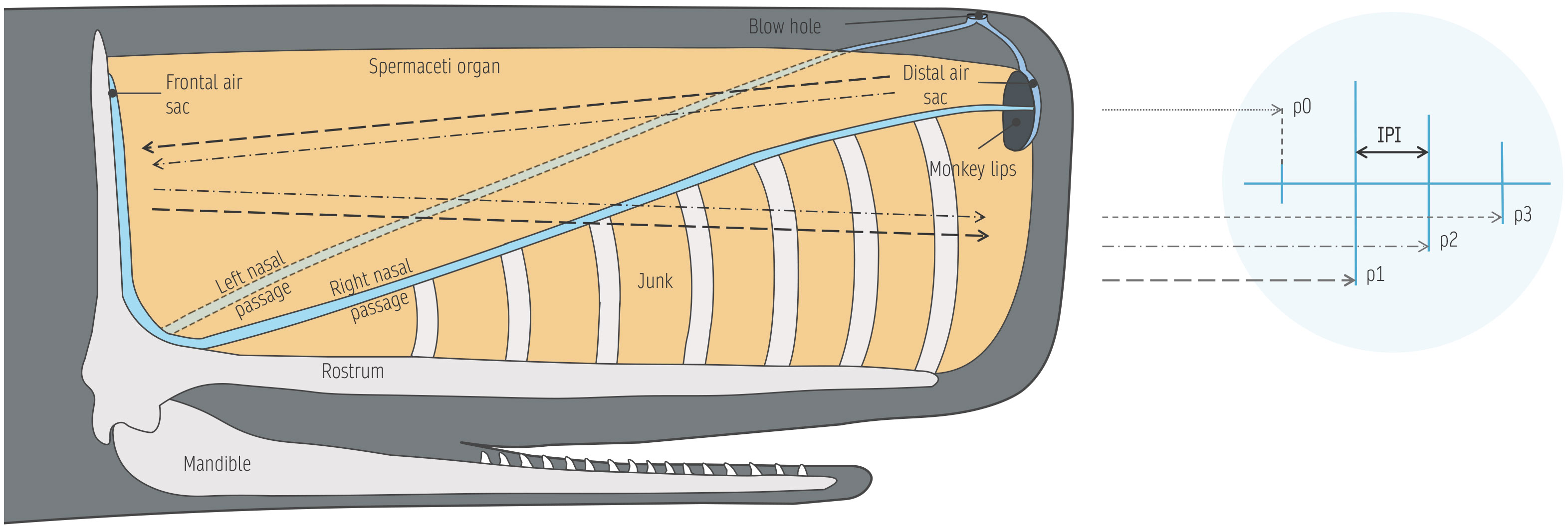
Figure 1 Anatomy of the sperm whale’s head and sound production pathway. Sperm whale clicks are composed of multiple, evenly spaced pulses (p0, p1, p2, p3).

In the accepted ‘bent-horn’ model (Møhl et al., 2003), after pneumatic production by the museau de singe (or monkey lips) located at the forefront of the head, 90% of the sound energy is reflected off the distal air sac and travels backwards through the spermaceti organ, while the remaining 10% exits frontally into the water from the top of the forehead, generating the low amplitude p0 pulse (Zimmer et al., 2005; Figure 1). The backwards-propagating fraction of energy is reflected back by the frontal air sac and travels forward through the junk organ, to finally be emitted from its lower part as the most powerful pulse; p1 (Figure 1). After the initial reflection off the frontal air sac, a fraction of the sound energy keeps travelling through the spermaceti organ, bouncing back and forth between the distal and frontal air sacs, generating successive pulses of decreasing amplitude, exiting from the lower junk (p2, p3, etc.) (Zimmer et al., 2005; Figure 1). Since those pulses have the same propagation path, the interval separating individual pulses (referred to as inter-pulse interval, or IPI) is stable, as it matches the two-way travel time between air sacs, reflecting the distance between them. Since the allometric relationship between the sperm whale’s head and total body length has been established from whaling studies (Nishiwaki et al., 1963), an individual’s size can be derived from IPIs (Adler-Fenchel, 1980; Gordon, 1991; Growcott et al., 2011; Caruso et al., 2015) based on sound speed profiles within the spermaceti organ (Flewellen and Morris, 1978).

Unfortunately, however, the high directionality of sperm whale clicks complicates the task. Depending on the position of the receiver relative to the whale’s acoustic axis, extra pulses appear at variable locations, altering the structure of the click in frequency and time, impeding the recognition of a stable IPI (Møhl et al., 2003; Zimmer et al., 2005). Optimal results are therefore obtained from recordings said to be ‘on-axis’, with the receiver located either directly in front or behind the whale. As a consequence, only a small fraction of clicks in a recording will show the desired multi-pulse structure, suitable for IPI measurement (Adler-Fenchel, 1980; Gordon, 1991; Rhinelander and Dawson, 2004). To overcome this issue, a lot of studies have manually searched and removed off-axis clicks (e.g. Adler-Fenchel, 1980; Gordon, 1991; Drouot et al., 2004; Schulz et al., 2011), which is effective but very strenuous considering the high click rate of sperm whales. Alternatively, averaging clicks in a sequence is a good solution for clicks produced by the same whale (Teloni et al., 2007; Antunes et al., 2010). But this requires click trains from different whales to be isolated, which is often very difficult to resolve (Beslin et al., 2018).

In this study, a tool based on machine recognition of on-axis clicks recently developed by Beslin et al. (2018), was used to process a heavy load of acoustic data collected in Irish offshore waters using static recorders and towed hydrophone arrays (Berrow et al., 2018). Barile et al. (2021) found that sperm whale clicks were detected on 79% of the days monitored with the static recorders, while Gordon et al. (2020) have estimated a density of 3.2 individuals per 1,000 km² based on the towed array data. Such numbers emphasise the significance of the region for sperm whales. Particularly, the majority of those animals are likely to be males, given the demographic habitat segregation characteristic of the species (Whitehead, 2018), with females rarely encountered north of 45° in the northeast Atlantic (Evans, 1997). Given the size composition of sperm whale populations found in the Azores (known breeding grounds; Steiner et al., 2012; Silva et al., 2014; van der Linde and Eriksson, 2020) and that in high-latitude feeding grounds such as northern Norway or Iceland (Lettevall et al., 2002; Madsen et al., 2002; Teloni et al., 2008), the most common expectation is for a population mostly dominated by large males in Irish waters, given the documented migrations of males between these grounds (Steiner et al., 2015). Catches from whaling stations seemed to support this hypothesis (Ryan, 2022), as well as stranding events in the area and around the British Isles, which are in majority represented by rather large males (Berrow and Rogan, 1997). Bachelor pods, composed of younger, maturing males are known to occur at these latitudes (O’Callaghan et al., in press) but are not expected to dominate the population. Considering the seemingly increasing numbers of stranding events involving females and calves (Berrow and Rogan, 1997; Berrow and O’Brien, 2005; O’Connell and Berrow, 2018), there is a necessity to shed more light on the structure of the population.

The implications of obtaining size-classes estimates of the sperm whale population are six-fold: (1) it will provide more reliable information on the actual structure of the population, which is an important step towards understanding the ecology of the species. Size information will allow us to infer the maturity stages/sexes of the animals present, helping to understand the relative importance of the area depending on group composition. In addition, (2) it will provide a baseline to monitor changes in size structure throughout the years, which could (3) suggest the existence of disturbances susceptible to affect individuals and (4) be used as a proxy for distribution shifts in response to changing environmental conditions such as warming temperatures. This is particularly important in the context of climate change, especially considering that sperm whales have already been shown to be expanding their range to colder, polar waters (Storrie et al., 2018; Popov and Eichhorn, 2020; Posdaljian et al., 2022) and highlighted as a species of high sensitivity potential to rising temperatures (Sousa et al., 2019; Peters et al., 2022). Finally, given the sexually dimorphic social structure of the species and the strong social units formed by females contrasting with the solitary behaviour of mature males, insights into population size-structure have the potential to (5) suggest intrinsic biological factors that could affect spatial distribution and habitat use (e.g. social interactions; Whitehead and Rendell, 2004; Eguiguren et al., 2019; Pirotta et al., 2020). Ultimately, (6) such information would be crucial to adapt and develop more appropriate management and conservation strategies.

2 Materials and methods

2.1 Data collection

This study exploits a large acoustic dataset collected between 2014 and 2016 in shelf break waters off western Ireland using both towed hydrophone arrays and bottom-mounted autonomous acoustic recorders (Figure 2). A brief description of the methods and instruments used for both acoustic monitoring techniques is given in the next sections. More details can be found in Gordon et al. (2020) for the towed arrays, and in Barile et al. (2021) for the static monitoring.

Figure 2

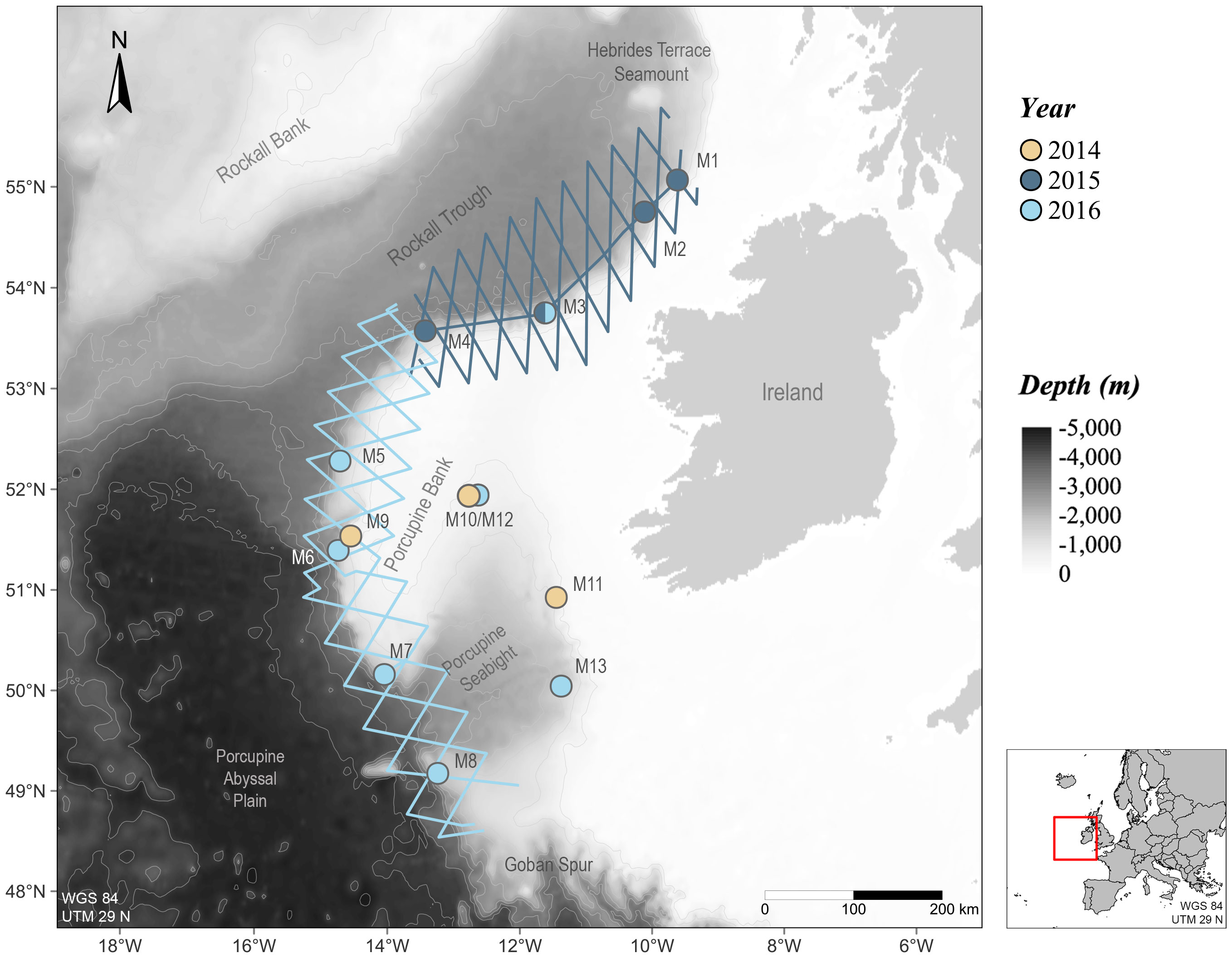
Figure 2 Acoustic monitoring along the Irish Atlantic Margin between 2014 and 2016. Thirteen static acoustic recorders (points) were deployed in 2014, 2015 and 2016 and six towed hydrophone arrays (lines) were carried out in 2015 and 2016.

2.1.1 Towed hydrophone array

Six towed hydrophone surveys were carried out as part of the ObSERVE Acoustic project (Berrow et al., 2018) along transect lines following a zig-zag survey design across slope areas in spring (May 2015 and 2016), summer (August 2015, June 2016) and autumn (September 2015, October 2016). Two surveys (May 2015 and 2016) were carried out from the RV Celtic Voyager, a 31 m research vessel operated by the Marine Institute (Ireland), while the other four transects were surveyed from the RV Song of the Whale, a 21 m motor sailing vessel operated by Marine Conservation Research (UK). Using a towed hydrophone array (Vanishing Point Ltd, Plymouth, UK), cetacean presence was monitored acoustically along transect, at an average travelling speed of 8 kn. A 340 m Kevlar-strengthened cable was used to tow a 10 m oil-filled streamlined section containing four hydrophone elements: a pair of ‘low frequency’ elements and preamplifier units (Benthos AQ4 with Magrec HP02 preamplifiers, 50 Hz low cut filter), spaced by 7 m and a pair of ‘high frequency’ elements and preamplifiers (Magrec HP03, 2 kHz low cut filter), placed 50 cm apart. For the high and low frequency elements with their associated preamplifiers, nominal frequency responses were of 2 kHz to 200 kHz and 50 Hz to 40 kHz, respectively. All hydrophone elements were connected on deck to a four-channel SAIL data acquisition card (St Andrews Instrumentation Ltd, Tayport, UK) set to sample at 500 kHz and data were written to hard disk drives as .wav files using the software PAMGuard (Gillespie et al., 2008, available at http://www.pamguard.org).

2.1.2 Static monitoring

Thirteen stations were monitored using bottom-mounted recorders located along the western slopes of the Porcupine Bank and in the Porcupine Basin (Figure 2). In 2014, three stations were monitored using the Wildlife Acoustic SM2 electronics, as part of a Woodside Energy (Ireland) Pty Ltd, Azeire Petroleum and Petrel Resources funded project (McCauley, 2015): stations M9 and M11 were equipped with HTI-99-HF omnidirectional hydrophones (High Tech, −204 dB re 1 V/µPa sensitivity) and station M10 with a Reson TC 4033 omnidirectional hydrophone (Teledyne Marine, −203 dB re 1 V/µPa sensitivity). The sampling rate was set to 192 kHz. In 2015 and 2016, Autonomous Multichannel Acoustic Recorders (AMARs; JASCO Applied Science) were deployed as part of the ObSERVE-Acoustic project (Berrow et al., 2018). AMAR units were equipped with omnidirectional HTI-99-HF (−164 dB re 1 V/µPa sensitivity) and M36-V35-100 (GeoSpectrum, −165 dB re 1 V/µPa sensitivity) omnidirectional hydrophones in 2015 (M1 to M4) and 2016 (M5 to M8, M12 and M13), respectively. High-frequency channels of all AMAR units were set to sample at 250 kHz. Recorders were duty cycled over different recording schedules (see Barile et al., 2021). Most units were suspended approximately 15 m above the seafloor (average operating depth of approx. 1,560 m), with the exception of devices at M9 and M11, deployed higher in the water column. All stations were equipped with acoustic releases for retrieval.

2.2 Data processing

Audio files (.wav) were all processed in CABLE (Cachalot Automatic Body Length Estimator), a free fully automated software developed by Beslin et al. (2018) to estimate IPIs from on-axis sperm whale clicks. CABLE was developed as a standalone application (exclusively available for Windows operating systems) in MATLAB environment, but only requires an installation of MATLAB Runtime R2015a (8.5; The MathWorks, Inc., Natick, Massachusetts). A thorough description of the software and its underlying algorithms was published by the developer in Beslin et al. (2018). The main steps are summarised below and in Figure 3.

Figure 3

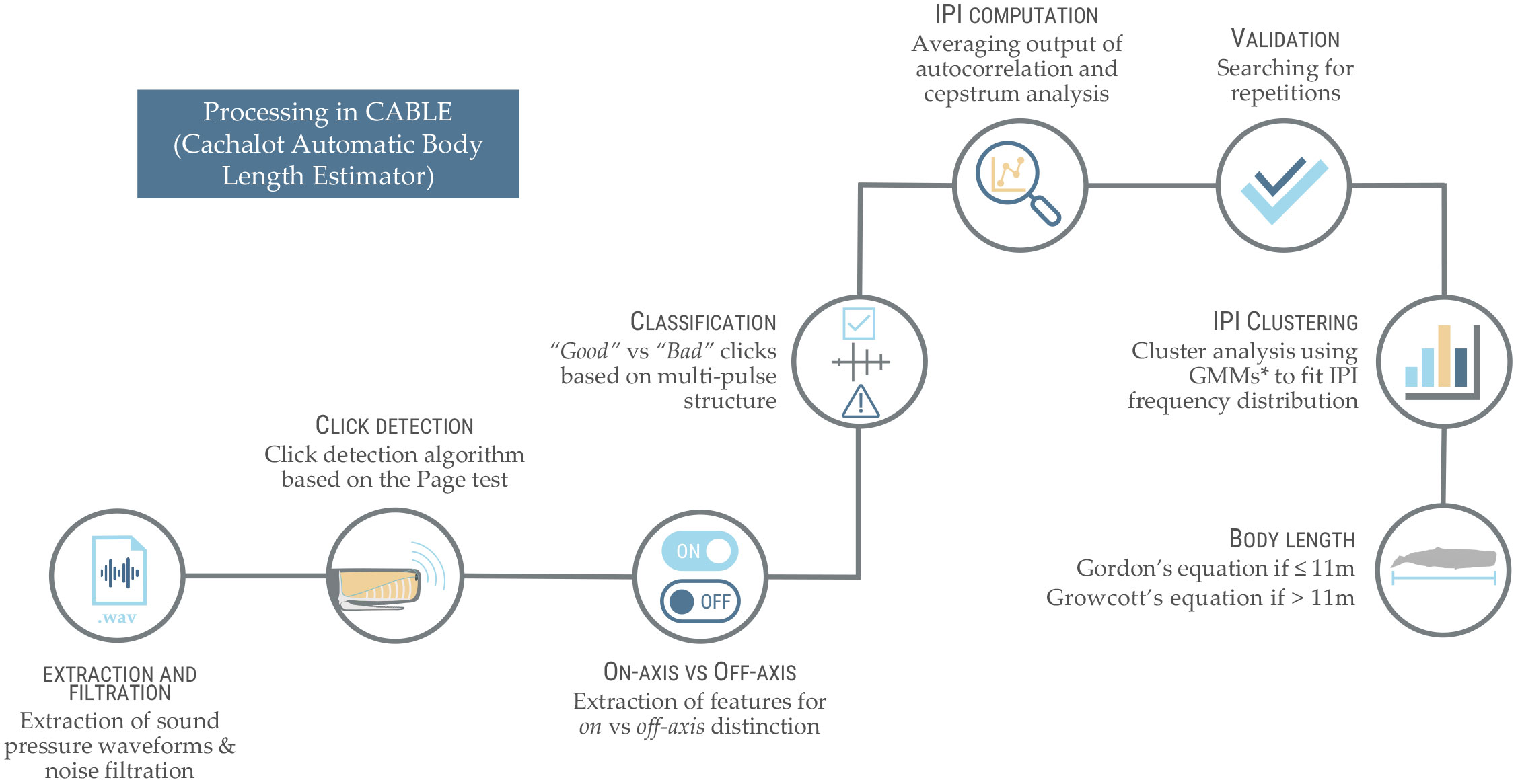
Figure 3 Summary of the main steps implemented in the automated software CABLE (Cachalot Automatic Body Length Estimator; developed by Beslin et al. (2018)) and used to derive sperm whale body lengths from the raw acoustic recordings in this study. *GMM, Gaussian Mixture Models.

After (1) first being extracted from audio input files, sound pressure waveforms are noise-filtered using a 2-12 kHz Butterworth bandpass filter to then (2) be scanned for clicks using a custom click detection algorithm based on the commonly used Page test (Page, 1954). The click detection routine implemented in CABLE is also used in PAMGuard (Gillespie et al., 2008), and was adapted to optimise the capture of the multipulsed structure of sperm whale clicks. Once candidate clicks are detected, (3) a set of features allowing the distinction of on-axis from off-axis clicks are extracted for each single click (following the prior computation of information necessary to those features, such as the location of individual pulses based on signal smoothing and the detection of local maxima, the frequency spectra of clicks and exponential curve fits describing the decay in amplitude of pulses). Some of those features are commonly used to characterise odontocete clicks (e.g., click duration, bandwidths, peak/centroid frequency) while others are especially suitable to the detection of the multipulsed nature of sperm whale clicks (e.g., pulse count, duration and variance, variance of zero-crossing rates, goodness of exponential fit to pulse peaks). In total, sixteen features are extracted and used in the routine (see Beslin et al., 2018, Table AI). Based on these, clicks are then (4) classified as being “Good” or “Bad” on-axis clicks. It is important to note here that only echolocation clicks can be considered Good. Bad clicks include non-sperm whale transients, off-axis and confounded on-axis clicks, surface reflections and coda clicks. Codas are classified as Bad because their structure (Madsen et al., 2002) and IPI (Schulz et al., 2011) significantly differ from that of echolocation clicks. The identification of Good clicks is based on the clear multipulsed waveform characteristic of on-axis clicks (Zimmer et al., 2005). Clicks are accepted if their probability of being Good is above 0.7 (default threshold). The next step (5) consists of the IPI computation for all clicks classified as Good. For more reliability, the algorithm computes the IPI using both an autocorrelation analysis and cepstrum analysis (Goold, 1996) and averages their outputs. Clicks for which the IPI estimates obtained with these methods were too different from one another (i.e., if IPI estimates deviate by > 0.05 ms from the average), were rejected (Schulz et al., 2011). An important point here is that for both methods, CABLE limits IPI calculations between 2-9 ms, which could exclude clicks produced by young calves (Tønnesen et al., 2018). Nevertheless, these thresholds recommended by Marcoux et al. (2006) are important, because allowing IPI calculations below 2 ms can lead to inaccurate results, while 9 ms is an upper limit for large males (Beslin et al., 2018).

Once IPIs calculated and precision verified, a final validation step is undertaken, based on a search for (6) IPI repetitions. Given that sperm whales emit clicks in trains, within a few seconds the same IPI is expected to be recorded more than once. Based on this property, the routine implemented in CABLE scans the time series forwards and backwards from each retained Good clicks’ time of occurrence, looking for another click with the same IPI ( ± 0.05 ms). From each successful scan, another follows, depending on the number of repetitions specified as needed to validate an IPI. The default value is set at 1, which implies that a click’s IPI must be repeated at least once to be validated (Beslin et al., 2018).

Finally, (7) from the filtered IPI distribution obtained, the number of whales and their body lengths are estimated. To this end, CABLE performs a cluster analysis using Gaussian mixture models (GMMs) to fit the frequency distribution of the filtered IPIs. This is based on the fact that IPIs from individual whales have been found to be rather stable (± 0.05 ms; Antunes et al., 2010; Growcott et al., 2011; Schulz et al., 2011). This implies that IPI distributions should contain a mixture of peaks, each of those corresponding to a single whale, which therefore assumes distinct IPIs for each whale of the recording. However, this could not be verified in our data, which is why this study cannot be used to estimate the number of animals recorded. For a single recording, IPIs from different animals of the same size (IPI differing by less than ±0.3 ms) were merged as one unique value, making the individual whales indiscernible. On the other hand, across recordings, if the same animal was to be recorded and its IPI to pass all filters, this would have gone unnoticed and this animal counted several times. The results of the GMM clustering provided the mean of each cluster present in a GMM, which corresponded to an estimate of a whale’s true IPI. If several GMMs with different numbers of clusters were computed, the routine compared them to one another using a Bayesian Information Criterion (BIC). Given the scale of our analysis, the model with the smallest BIC value was automatically selected for each subset analysed (see the following section for details on subsets).

A number of parameters used by the CABLE routine can be adjusted by the user in specific cases, but default parameters are recommended and considered robust to most scenarios (Beslin et al., 2018). In this study, the advice was followed and all parameters maintained to their default setting.

2.3 Data analysis

To have a chance of investigating differences in both space and time and considering the strictness of CABLE’s routine (99% of the candidate clicks are likely to be rejected; Beslin et al., 2018, CABLE User Guide), the entire dataset available was processed. Since all data came from far-field recordings, we did not expect a daily or even weekly resolution to yield significant IPI distributions. Moreover, given our research questions, such a fine temporal resolution was not necessary. For these reasons, the sound files were organised in monthly folders for each monitoring station, and by transect for each towed array survey. When processing audio files, CABLE generates outputs for each corresponding sub-folder (here for each month and station, or each transect). These outputs can be of three types: all detected clicks (result of step (2) as described above), filtered clicks (result of step (6)), results of clustering analysis (result of step (7)). Any of those files can be requested prior to initiating the routine. All mean IPIs resulting from clustering analysis were extracted and merged into a single dataset and matched to the station/transect where they were recorded. This final dataset was then imported into R (v. 4.1.2; R Core Team, 2018) for visualisation and analysis.

The relationship between stable IPIs and the size of a sperm whale’s head has been widely documented, as well as the allometric relationship between head and body length (Clarke, 1978; Møhl et al., 1981; Gordon, 1991; Jaquet, 2006; Growcott et al., 2011). Gordon (1991) used measurements of sperm whales obtained via photogrammetry to propose an empirical relationship (Equation 1) between IPIs and body length, as follows:

$\begin{array}{ll}BL=4.833+1.453\ast IPI-0.001\ast IP{I}^2& (1)\end{array}$

This equation was mainly tested on juvenile sperm whales, with the exception of one individual larger than 12 m (Gordon, 1991). As a result, Gordon’s equation is considered very reliable for animals ≤11 m (Madsen et al., 2002; Caruso et al., 2015). For whales larger than 11 m, a new equation was then proposed by Growcott et al. (2011), as follows (Equation 2):

$\begin{array}{ll}BL=1.258\ast IPI+5.736& (2)\end{array}$

Both of the above equations were used to derive individuals’ body length (BL) from the mean IPIs computed by CABLE for each cluster. Support for the combination of those two equations and for the exclusion of a recent refinement of Growcott’s equation (Dickson et al., 2021) is given is Supplementary Material (Supplementary Figure S1). The general size-frequency distribution was computed for the entire monitored area across all sampling periods. In addition, the body lengths were assigned to the three following classes, as suggested by Caruso et al. (2015) on the basis of growth curves established by Rice (1989). This allowed us to provide information on the proportions of the respective classes.

● Immature individuals (male or female): BL < 9 m;

● Adult females or juvenile males: BL = 9-12 m;

● Adult males: BL > 12 m.

In addition, an exploration of potential differences in size-frequency distributions across recording locations/surveys was undertaken. PAM transects from the same area/year were grouped into north (surveyed in 2015) and south (surveyed in 2016) blocks, given their short duration and the low amount of stable IPIs extracted from individual surveys. Some stations/transect blocks had low numbers of IPI clusters and were therefore not considered in subsequent analysis. The threshold for inclusion was set to thirty IPI estimates, which were deemed necessary for a distribution to be observed (see Supplementary Figure S2). Following the application of this threshold, the south block of PAM transects (surveyed in 2016) as well as stations M9, M10 and M11 were excluded. Due to a lack of spatio-temporal replicates in the data, potential confounding factors needed to be isolated prior to investigating spatial differences in body lengths. Firstly, sperm whale body lengths derived from towed array and static monitoring data were compared using a Wilcoxon signed rank test, to ensure the method of data collection did not influence the results. Secondly, the effect of the recording year was also investigated (using the same test) to determine whether results from either year could be compared or if they should be separated. It is however important to note that the survey design did not allow to disentangle an effect of the year from a spatial effect, given that (except at M3, where monitoring occurred both in 2015 and 2016, yet at different times of the year) the northern part of the area was monitored in 2015 while the southern part was monitored in 2016. Two separate one-way ANOVAs were then used to investigate spatial differences in mean sperm whale body length among stations monitored in 2015 and among those monitored in 2016. Since CABLE limited IPI calculations between 2-9 ms, a truncated regression was used to model sperm whale body length using the function truncreg() from the truncreg library (Croissant and Zeileis, 2016). The truncation point was set to the minimum size of 7.74 m (corresponding to an IPI of 2.00 ms). Subsequently, to pinpoint between which stations the body lengths were significantly different within each year, a Tukey-Kramer test was used. All analysis and data visualisation were carried out using R (R Core Team, 2018). To determine statistical significance, a threshold α = .05 was used.

3 Results

Over 10,000 hours of acoustic recordings (∼9,000 hours collected using static devices and ∼1,000 hours collected using towed arrays) were processed in CABLE. The initial dataset generated by the click detection algorithm implemented in the routine contained a total of 34,528,036 candidate clicks, of which IPIs were extracted. Out of those, 75,437 (0.2%) passed all validation steps (classification, precision and repetition). Finally, the cluster analysis applied to the filtered IPI distribution yielded 1,594 clusters (corresponding to as many individual whales), from which mean IPIs were extracted. Note that given the spatio-temporal coverage of the data processed, instruments and algorithms used, as well as the mobility of sperm whales, the same animals might have been measured at different periods and locations. However, the chance of obtaining duplicate estimates for a single whale can be considered the same across size classes, and would not have affected the estimates. That said, the results presented here should under no circumstance be used to infer abundance estimates. IPIs measurements ranged between 2.00 to 8.76 ms (mean IPI = 4.08 ms, sd = 1.48 ms). Summary statistics for each station/transect monitored are given in Table 1. Note the discrepancies in sample sizes and the absence of stable IPIs at M11.

Table 1

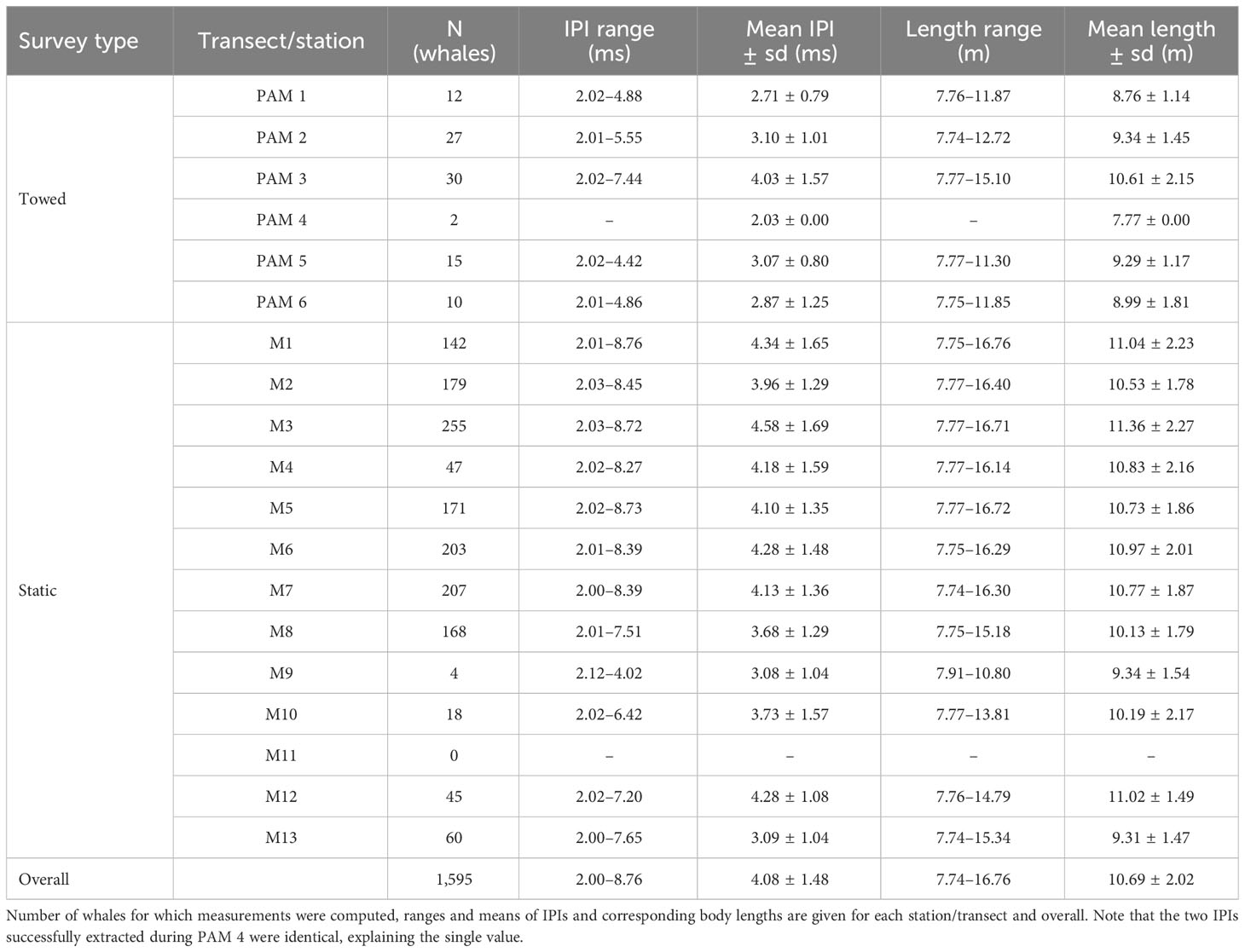
Table 1 Summary of IPIs and corresponding length estimates of recorded whales.

The estimated length of the whales recorded over the whole area and study periods ranged from 7.74 to 16.76 m (mean length = 10.69 m, sd = 2.02 m, median = 10.48 m; Table 1 and Figure 4). The largest whale (16.76 m) was recorded in October 2015 to the northernmost point of the study area (station M1; Figure 2), while the smallest was recorded in July 2016 in the south of the area (station M13). The classification of the recorded animals into different sex/maturity stages based on the estimated body lengths revealed that adult females/juvenile males (body length of 9-12 m) were predominant, accounting for 49% (n = 788) of the total number of recorded individuals (n = 1,595; Figure 4). The proportions of immature individuals and adult males were well balanced, accounting for 25% (n = 394) and 26% (n = 413) of the recorded whales, respectively. Within the 413 adult males, 19 whales (1% out of 1,595) were physically mature, with body lengths greater than 16 m (Whitehead, 2018).

Figure 4

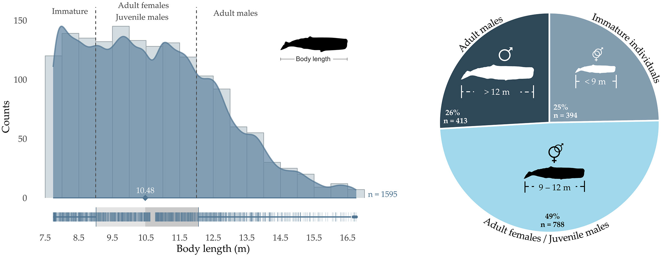
Figure 4 Sperm whale size-frequency distribution in Irish offshore waters. Histogram (left hand side) of sperm whale body length grouped in classes of 50 cm and density plot over the continuous interval of lengths. Dashed vertical lines delimit the hypothetical sex/maturity stage as described in Caruso et al. (2015). A boxplot is represented at the bottom of the figure, with vertical blue segments representing actual data points. The median (indicated by the diamond shape), first and third quartiles (vertical grey segments) are given, as well as the overall number of records (n). Estimated lengths are derived with Gordon’s equation for IPIs < 4 ms and Growcott’s equation for IPIs > 4 ms. Number and proportion (right hand side) of animals assigned to hypothetical sex/maturity stages. Note that within the adult males category, 19 individuals (1% of the overall number of individuals recorded) were larger than 16 m, size indicating physical maturity (Whitehead, 2018).

Our data provided statistical evidence of an effect of the recording method (towed arrays vs deep recorders) on extracted IPI values and resulting body lengths (Wilcoxon signed rank; P<.001). In particular, body lengths extracted from individuals recorded using deep recorders were significantly greater than those obtained from towed array surveys (Supplementary Figure S3). This bias prevented comparisons of body lengths across these different recording methods. Due to the scarcity of IPIs obtained from towed array surveys, comparisons across different surveys were abandoned (Table 1 and Supplementary Figure S2). In addition, we found statistical evidence that body lengths obtained from deep recorders’ data deployed in 2015 were significantly greater than in 2016 (Wilcoxon signed rank; P<.05 - Supplementary Figure S4). As previously mentioned, considering the sampling design, it is possible that rather than being due to the sampling year, this difference could reflect some spatial segregation in the area. By comparing body lengths of animals recorded within each year by means of one-way ANOVAs, we highlighted the existence of significant differences across stations monitored in 2015 (F(3, 482) = 7.26, P<.001), as well as between stations monitored in 2016 (F(6, 984) = 9.73, P<.001). Post-hoc Tukey-Kramer tests revealed that in 2015, recorded sperm whales significantly differed in length only between stations M2 and M3, with significantly larger animals at M3 (Figure 5). Detailed outputs of Tukey Kramer tests are given in Supplementary Material (Supplementary Figure S5).

Figure 5

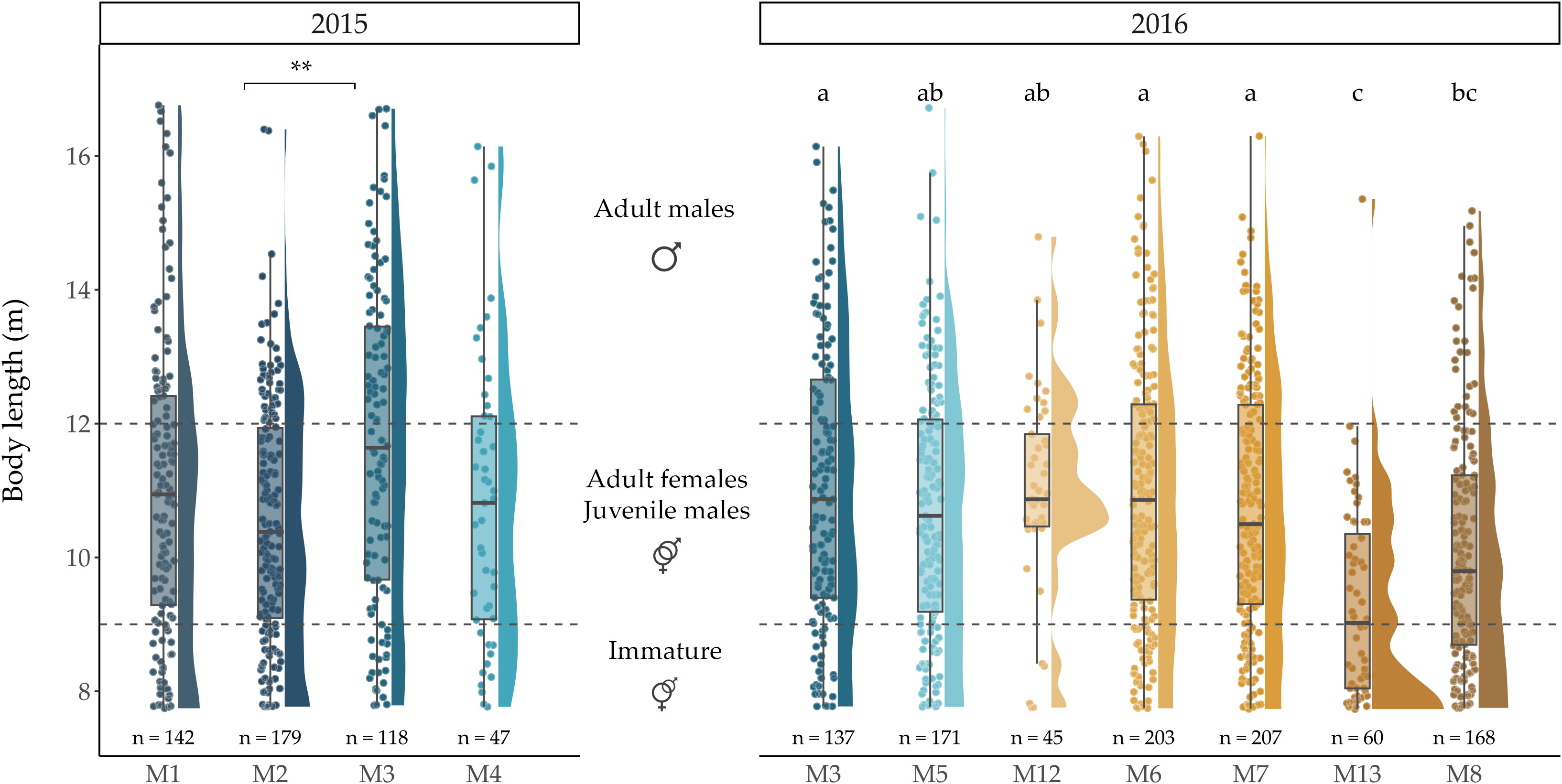
Figure 5 Sperm whale body lengths (m) per station. Statistical significance is indicated by asterisks for stations monitored in 2015 (left) and by a compact letter display for stations monitored in 2016 (right): mean body length between stations sharing the same letter do not significantly differ. The order of the stations on the x-axis reflects north to south location. Horizontal dashed lines delimit maturity stages/sex. Stations monitored in 2015 were compared independently from those monitored in 2016 due to differences in body lengths found across years.

An inspection of Figure 5 suggested a light trend towards gradually smaller animals from north to south (M3 to M8) in 2016. At M8 however, animals seemed larger than at M13, yet smaller than at all other stations. It is important to note here the particular location of M13 (Figure 2), on the eastern slopes of the Porcupine Seabight, whereas all other stations (with the exception of M12) were located on the western slopes of the Porcupine Bank. The Tukey-Kramer test revealed that animals at M13 were significantly smaller than animals at all other stations except M8 (Figure 5). Animals were also significantly smaller at M8 than at M3, M6 and M7. These results could suggest some degree of latitudinal segregation in body length in the area, but our data does not support clear conclusions and caution should be taken considering the unbalanced sample sizes in the comparisons, despite the conservative nature of the Tukey-Kramer tests.

4 Discussion

This study presented the first size-frequency distribution of sperm whales in Irish offshore waters. Despite their presence in numbers comparable to other areas considered as sperm whale concentrations (Gordon et al., 2020), very little is known about the composition of the population, even less so about its social structure. Male sperm whales have long been considered to dominate the Irish population (Wall et al., 2013), given the characteristic spatial segregation known to separate males from females and young (Whitehead et al., 2003). Females in the northeast Atlantic are rarely found at latitudes higher than 45° (Evans, 1997), which entails that the Irish population would be expected to be dominated by maturing to mature males. With the present study however, we demonstrated that immature individuals seem to be present in significant numbers off the west coast of Ireland. Our data showed that animals < 9 m in length accounted for a similar proportion of the recorded animals than adult males (> 12 m) did. In addition, an investigation of spatial differences suggested smaller individuals to be more present in the south of the area.

In the wider northeast Atlantic basin, females and young are known to inhabit the Azores, undertaking latitudinal migrations of around 1,500 km, towards other islands such as the Canaries (Steiner et al., 2015). Mature males are also found in the Azores, but in much lesser proportions, as highlighted by Steiner et al. (2012) who reported that only 10% of photo-identified animals between 1987 and 2008 were mature males. This large predominance of female social units (comprising adult females, juveniles and calves) was also confirmed by Silva et al. (2014) and van der Linde and Eriksson (2020). Up north, in feeding grounds such as in northern Norway, male sperm whales are dominant (Lettevall et al., 2002; Madsen et al., 2002; Teloni et al., 2008; Oliveira, 2014). Migration of male sperm whales between these high-latitude foraging grounds and the breeding grounds in the Azores was reported (Whitehead et al., 2003; Steiner et al., 2012), as well as matches based on whaler’s harpoons between the Azores and Iceland (Martin, 1982). Stranding records have also matched an individual stranded in Ireland in 1997 with a photo-identification image from Andenes, Norway (Steiner et al., 2012). However, no published data to date has reported evidence of a significant presence of female social units at such high latitudes. The absence of previous size-classes estimates in Irish waters precludes any direct comparison with our findings. As mentioned before, females and young are not known to migrate to latitudes higher than 40-45° (Hobbs et al., 2007). Apart from isolated stranding cases, no records of breeding individuals have been reported around the study area (Berrow and Rogan, 1997; Santos et al., 2006). Berrow and Rogan (1997) reported that nearly all (19 out of 20) sperm whale individuals (with definite gender identification) found stranded in Ireland were males. Data from whaling records can also give some interesting indications. In the northeast Atlantic, sperm whales were a regular target of whalers in Iceland, Norway, Scotland, Ireland, Portugal, Spain, the Azores and Madeira (Brown, 1976; Fairley, 1981; Tønnessen and Johnsen, 1982) and males were a common catch in the area and adjacent waters (Ryan, 2022). Fairley (1981) reported 63 males caught between 1908 and 1922 from the stations in western Mayo, Ireland and Brown (1976) reported 76 males caught in the Outer Hebrides, UK between 1904 and 1928. However, a lot of caution should be taken when using data derived from whaling logbooks, given that the reports were often biased towards larger, adult males.

With the present study we provided evidence that immature whales were present and represented a significant proportion of the recorded animals (25%). Adult males (> 12 m) accounted for only 26% of the animals recorded. Such findings suggest that Irish waters are important for animals at all maturity stages and seem to be an intermediate ground, with a more mixed population. The proportion of adult males is indeed lower than in Norway, yet higher than in the Azores. Male sperm whales can disperse from their matrilineal social units at any point between 4 and 21 years old (Whitehead et al., 2003) and form loose aggregations, often called ‘bachelor’ groups. Their latitudinal range can overlap that of the females and mature males (Best, 1979; Whitehead et al., 1989). Pods of young bachelors are known to occur around the area (O’Callaghan et al., in press), but were not thought to represent a part of the population as large as the one we reported here. The minimum length we reported here was of 7.74 m. This means that the immature individuals (< 9 m) recorded could have been individuals having either already left their units and travelled north, or been with their maternal units. The latter would imply that some of the 9-12 m animals were females. This possibility must not be excluded and has previously been suggested by O’Cadhla et al. (2004), who reported three sightings of calves in offshore Irish waters. Two calves also stranded in Ireland, in 1916 and 2004 (Berrow and O’Brien, 2005). In addition, nine confirmed females were also found, seven of which stranded since 2013 (Simon Berrow, 2022, pers. comm.; Berrow and Rogan, 1997; O’Connell and Berrow, 2018). Berrow and Rogan (1997) reported six individuals of lengths smaller than 12 m, out of 15 animals for which measurements were available. Recently, a female stranded in Wales, the fourth female to strand in the UK in the last century (Pinkstone, 2023). In addition, Hobbs et al. (2007) suggested that some breeding/calving grounds could exist in the Bay of Biscay, already at higher latitudes than previously thought.

Our results also suggested some level of latitudinal segregation within the surveyed area, with more immature whales in the south in comparison to the north, and vice-versa for adult males. Such an observation is not surprising given that, in the light of the data presented here, Ireland could be an intermediate between breeding grounds in the Azores, potentially in the Bay the Biscay (Hobbs et al., 2007) and established feeding grounds in Norway and higher latitudes. However, caution should be taken here, given the discrepancy in sample sizes. Interestingly though, more detailed investigations into distributions at individual stations revealed that the two southernmost stations were yielding significant differences (M13 and M8) with the rest of the area, with smaller animals than elsewhere.

In this study, recordings from both bottom-mounted and towed hydrophones were used. However, the number of stable IPIs obtained from towed hydrophone data was overall rather low. This could be due to the presence of surface reflections in detected clicks, an issue not applicable to clicks detected in recordings from bottom-mounted instruments. In early stages, the algorithm separates Good and Bad clicks, the latter including clicks contaminated by surface reflections which are therefore discarded. In addition, analyses suggested an effect of the type of methodology on the length estimates. A plausible hypothesis for this could lay in the overlap between animals of certain lengths and the instruments; deep recorders are less likely to pick up stable IPIs from animals undertaking shallower dives (i.e., smaller individuals), whereas surface instruments are themselves less likely to pick up large males, more solitary, undertaking deeper dives and silent during their ascent and surfacing periods.

The range of body lengths obtained in this study was in line with worldwide reported lengths of sperm whales and no alarming measurement was observed. In the western Atlantic, Adler-Fenchel (1980) reported IPIs ranging from 1.6 to 8.0 ms, corresponding to body lengths of 7.3 to 21.7 m based on the older equation from Møhl et al. (1981). However, using the equations of Gordon (1991) and Growcott et al. (2011) to recalculate minimum and maximum body lengths in that study, body lengths ranged from 7.2 to 15.8 m. In addition, several studies in the southern Pacific (New Zealand) have reported lengths between 12.5 to 15.5 m (Rhinelander and Dawson, 2004; Growcott et al., 2011; Giorli and Goetz, 2020). In the Mediterranean sea, Caruso et al. (2015) reported body sizes between 7.5 to 14 m and more recently, Marcolin (2021) reported lengths ranging from 7.79 to 14.56 m in the Azores. The measurements found here are therefore in accordance with previous studies using the same equations. It is important to mention that the CABLE routine limited calculation of IPIs between 2-9 ms (Beslin et al., 2018). The upper bound corresponds to a limit for the IPIs of large males. Since the maximum IPI value extracted here (8.76 ms) was lower than the upper bound, it will not have affected the detectability of larger males. However, the minimum IPI (2.01 ms) extracted was very close to the lower bound set by the routine. If younger calves (< 7.75 m) were present, they were not detected. This implies that the proportion of individuals classified as Immature could be underestimated, with individuals of even smaller size also present.

In order to obtain more reliable results, the decision to exclude stations/transects with a number of individual IPIs < 30 was taken. The choice of applying such a threshold was to remain conservative and limit the risk of single estimates skewing the distribution and leading to erroneous conclusions. A sample size of thirty was deemed to be sufficient to be representative of body length distributions, which could reliably be included in comparisons. Low sample sizes are indeed more likely to reflect a detection bias rather than an actual picture of size-classes, especially considering the strict nature of CABLE’s algorithms. Considering the latter, we can safely consider our findings to be reliable. We however warn the reader that under no circumstance should any whale count presented in this study be considered in the context of abundance or density estimates. The main advantage of CABLE is its capacity to distinguish on-axis and off-axis clicks in the recordings, which implies that click trains do not need to be resolved, as no prior knowledge regarding which vocalising whale is at the origin of the clicks is required (Beslin et al., 2018). It is precisely this feature that allowed such a large dataset consisting of far-field recordings to be processed. On-axis clicks require a specific orientation of the whale relative to the hydrophone, achieved on the field by following sperm whales using a towed hydrophone as part as dedicated surveys. In the case of recordings obtained from deep static recorders, the probability of obtaining suitable clicks is greatly reduced. In addition to requiring (1) the click to be on-axis, it also must be (2) clearly separated from other clicks and echoes and (3) the signal-to-noise ratio must be sufficiently high for the candidate click to be suitable for IPI computation (Beslin et al., 2018). The probability for a click to meet all these criteria is evidently extremely low for recordings obtained from deep static recorders. The additional strict classification thresholds explain the extremely low proportion of clicks passing through the filters (0.2% in this study). Marcolin (2021) tested CABLE on a small number of recordings from the Azores and compared the obtained measurements with those computed by the Sperm Whale IPI plugin (Miller et al., 2013) implemented in PAMGuard (Gillespie et al., 2008) and manually, to find that CABLE did not yield enough measurements. Here however, the large amount of data processed led to representative distributions at some stations. Given the strict filters in CABLE, the high number of false negatives comes together with an extremely low probability of false positives, which implies that every single computed IPI is likely to be highly reliable (Beslin et al., 2018). CABLE is a relatively recent tool, but Beslin et al. (2018) reported great performances of the routine. They highlighted a sensitivity (i.e., true positive rate) of 89.1%, a specificity (i.e., true negative rate) of 99.5% and a precision of 92.7% in terms of classification of on-axis sperm whale clicks from other transients. Based on these metrics, one can confidently rely on the extracted on-axis clicks. What was highlighted by Beslin et al. (2018) was the extremely low acceptance rate, with less than 0.01% of detected clicks accepted into the final IPI distributions. If this low acceptance rate can preclude the use of CABLE on small datasets (Marcolin, 2021), the focus placed on precision rather than recall mean that the obtained distribution are very reliable. Finally, it is important to add that the methods used to compute IPI distributions (i.e., cross-correlation and cepstrum analyses) have long been established, tested and used in many studies (e.g. Goold, 1996; Pavan et al., 1997; Teloni et al., 2007; Antunes et al., 2010; Caruso et al., 2015). However, it is important to note that CABLE was trained on data consisting predominantly of social units (females and young), making a bias towards this size-group conceivable (Wilfried Beslin, 2023, pers. comm.). Therefore, manually calculating IPIs on a suitable subset of the dataset used here and comparing them with the output of CABLE would add robustness to the results. Further, our data could be incorporated into the training dataset of CABLE, to increase the applicability of the routine.

Very recently, Solsona-Berga et al. (2022) have shown that inter-click-intervals (ICIs; measure of the echolocation repetition rate) and IPIs were linearly correlated, allowing body lengths to be estimated based on ICIs. Their innovative approach by-passes the apparent bias associated with the behaviour-induced modulations in ICIs, occurring within a single dive (Thode et al., 2002; Zimmer et al., 2003; Teloni et al., 2008), opening new possibilities of measuring sperm whales acoustically. Using ICIs instead of IPIs considerably increases the amount of exploitable clicks in recordings, given that off-axis clicks could be used, which means that size estimates could be obtained with far less data. A comparison of results obtained using the tool from Beslin et al. (2018) (used here) and with the approach developed by Solsona-Berga et al. (2022) would be an interesting investigation in the future.

Visual encounters with sperm whales in favourable weather conditions are rare in Irish waters. Sperm whales in Ireland are found relatively far off the coast, along the continental slopes, an area not only challenging to survey with traditional visual methods, but expensive. This explains the lack of photogrammetry or photo-identification data that would allow a better understanding of the structure of the sperm whale population. Here we demonstrated the great value of acoustic datasets, especially in the context of an ongoing development of automatic algorithms for detection and classification, along with the growing popularity of machine learning. The large dataset exploited allowed us to extract a sufficient number of IPIs to estimate the size structure of the Irish population for the first time. By creating an important baseline, this study will allow researchers to track changes in the distribution of this emblematic species, likely to be particularly sensitive to climate change (Sousa et al., 2019; Peters et al., 2022). In addition, shedding light on the structure of the population is an important step towards better understanding its ecology and habitat use relative to group composition, invaluable information for conservation and management strategies (Pirotta et al., 2011; Pace et al., 2018; Eguiguren et al., 2019; Pirotta et al., 2020).

Data availability statement

Publicly available datasets were analyzed in this study. This data can be found here: https://www.gov.ie/en/publication/12374-observe-programme/#project-data.

Author contributions

CB: Conceptualization, Data curation, Formal analysis, Investigation, Methodology, Software, Validation, Visualization, Writing – original draft. SB: Funding acquisition, Project administration, Resources, Supervision, Writing – review & editing. JO’B: Funding acquisition, Project administration, Resources, Supervision, Writing – review & editing.

Funding

The author(s) declare financial support was received for the research, authorship, and/or publication of this article. This research could be finalised thanks to CB’s Irish Research Council Postdoctoral Fellowship (award number GOIPD/2022/446). Preliminary analyses and drafts of this research were carried out as part of CB’s PhD thesis, funded by the Atlantic Technological University and Woodside Energy Ltd. The data used here is part of a Woodside Energy Ltd. study and the ObSERVE Acoustic project, initiated and funded by the Department of Communications, Climate Action and Environment in partnership with the Department of Culture, Heritage and the Gaeltacht under Ireland’s ObSERVE Programme. We are extremely grateful to the Marine Institute (Ireland) for awarding a Networking Initiative (NET/23/036) to CB to cover publication fees. The Networking Initiative is funded by the Marine Institute under the Marine Research Programme with the support of the Irish Government. The funder Woodside Energy Ltd. was not involved in the study design, analysis, interpretation of data, the writing of this article or the decision to submit it for publication.

Acknowledgments

Very special thanks to W. Beslin for his opinion and suggestions on this manuscript. We thank C. Minto, M. Pommier, S. Gero, J. Gordon and S. O’Callaghan for their advice on different aspects of this work on earlier stages. We also thank the three reviewers who contributed to the improvement of this manuscript.

Conflict of interest

The authors declare that the research was conducted in the absence of any commercial or financial relationships that could be construed as a potential conflict of interest.

Publisher’s note

All claims expressed in this article are solely those of the authors and do not necessarily represent those of their affiliated organizations, or those of the publisher, the editors and the reviewers. Any product that may be evaluated in this article, or claim that may be made by its manufacturer, is not guaranteed or endorsed by the publisher.

Supplementary material

The Supplementary Material for this article can be found online at: https://www.frontiersin.org/articles/10.3389/fmars.2023.1264783/full#supplementary-material

References

Adler-Fenchel H. S. (1980). Acoustically derived estimate of the size distribution for a sample of sperm whales (Physeter catodon) in the western North Atlantic. Can. J. Fisheries Aquat. Sci. 37, 2358–2361. doi: 10.1139/f80-283

CrossRef Full Text | Google Scholar

Antunes R., Rendell L., Gordon J. (2010). Measuring inter-pulse intervals in sperm whale clicks: Consistency of automatic estimation methods. J. Acoustical Soc. America 127, 3239–3247. doi: 10.1121/1.3327509

CrossRef Full Text | Google Scholar

Backus R. H., Schevill W. E. (1966). “Physeter clicks,” in Whales, dolphins and porpoises. Ed. Norris K. S. (Berkeley: University of California Press), 510–528.

Google Scholar

Barile C., Berrow S., Parry G., O’Brien J. (2021). Temporal acoustic occurrence of sperm whales Physeter macrocephalus and long-finned pilot whales Globicephala melas off western Ireland. Mar. Ecol. Prog. Ser. 661, 203–227. doi: 10.3354/meps13594

CrossRef Full Text | Google Scholar

Berrow S. D., O’Brien J. (2005). Sperm whale Physeter macrocephalus L. calf, live stranded in Co Clare. Irish Naturalists J. 28, 40–41.

Google Scholar

Berrow S., O’Brien J., Meade R., Delarue J., Kowarski K., Martin B., et al. (2018). Acoustic Surveys of Cetaceans in the Irish Atlantic Margin in 2015–2016: Occurrence, distribution and abundance. Tech rep (Department of Communications, Climate Action and Environment and the National Parks and Wildlife Service (NPWS), Department of Culture, Heritage and the Gaeltacht).

Google Scholar

Berrow S., Rogan E. (1997). Review of cetaceans stranded on the Irish coast 1901-1995. Mammal Rev. 27, 51–75. doi: 10.1111/j.1365-2907.1997.tb00372.x

CrossRef Full Text | Google Scholar

Beslin W. A. M., Whitehead H., Gero S. (2018). Automatic acoustic estimation of sperm whale size distributions achieved through machine recognition of on-axis clicks. J. Acoustical Soc. America 144, 3485–3495. doi: 10.1121/1.5082291

CrossRef Full Text | Google Scholar

Best P. B. (1979). “Social organisation in sperm whales, Physeter macrocephalus,” in Behavior of marine mammals. Eds. Winn H. E., Olla B. L. (Boston, MA: Springer), 227–289. doi: 10.1007/978-1-4684-2985-57

CrossRef Full Text | Google Scholar

Brown S. (1976). Modern whaling in Britain and the north-east Atlantic Ocean. Mammal Rev. 6, 25–36. doi: 10.1111/j.1365-2907.1976.tb00198.x

CrossRef Full Text | Google Scholar

Caruso F., Sciacca V., Bellia G., Domenico E. D., Larosa G., Papale E., et al. (2015). Size distribution of sperm whales acoustically identified during long term deep-sea monitoring in the Ionian Sea. PloS One 10, e0144503. doi: 10.5281/zenodo.33202

PubMed Abstract | CrossRef Full Text | Google Scholar

Christiansen F., Sironi M., Moore M. J., Di Martino M., Ricciardi M., Warick H. A., et al. (2019). Estimating body mass of free-living whales using aerial photogrammetry and 3D volumetrics. Methods Ecol. Evol. 10, 2034–2044. doi: 10.1111/2041-210X.13298

CrossRef Full Text | Google Scholar

Clarke M. R. (1978). Structure and proportions of the spermaceti organ in the sperm whale. J. Mar. Biol. Assoc. United Kingdom 58, 1–17. doi: 10.1017/S0025315400024371

CrossRef Full Text | Google Scholar

Cranford T. W. (1999). The sperm whale’s nose: Sexual selection on a grand scale? Mar. Mammal Sci. 15, 1133–1157. doi: 10.1111/j.1748-7692.1999.tb00882.x

CrossRef Full Text | Google Scholar

Croissant Y., Zeileis A. (2016). truncreg: truncated gaussian regression models. Available at: https://CRAN.R-project.org/package=truncreg.

Google Scholar

Dickson T., Rayment W., Dawson S. (2021). Drone photogrammetry allows refinement of acoustically derived length estimation for male sperm whales. Mar. Mammal Sci. 37 (3), 1150–1158. doi: 10.1111/mms.12795

CrossRef Full Text | Google Scholar

Dillingham P. W., Moore J. E., Fletcher D., Cortés E., Curtis K. A., James K. C., et al. (2016). Improved estimation of intrinsic growth rmax for long-lived species: integrating matrix models and allometry. Ecol. Appl. 26, 322–333. doi: 10.1890/14-1990

PubMed Abstract | CrossRef Full Text | Google Scholar

Douglas L. A., Dawson S. M., Jaquet N. (2005). Click rates and silences of sperm whales at Kaikoura, New Zealand. J. Acoust. Soc. Am. 118, 523–529. doi: 10.1121/1.1937283

PubMed Abstract | CrossRef Full Text | Google Scholar

Drouot V., Gannier A., Goold J. C. (2004). Diving and feeding behaviour of sperm whales (Physeter macrocephalus) in the Northwestern Mediterranean Sea. Aquat. Mammals 30, 419–426. doi: 10.1578/am.30.3.2004.419

CrossRef Full Text | Google Scholar

Eguiguren A., Pirotta E., Cantor M., Rendell L., Whitehead H. (2019). Habitat use of culturally distinct Galapagos sperm whale Physeter macrocephalus clans. Mar. Ecol. Prog. Ser. 609, 257–270. doi: 10.3354/meps12822

CrossRef Full Text | Google Scholar

Evans P. (1997). Ecology of sperm whales (Physeter macrocephalus) in the eastern North Atlantic, with special reference to sightings and strandings records from the British Isles. Biologie Unserer Zeit 67, 37–46.

Google Scholar

Fairley J. (1981). Irish whales and whaling (Belfast: Blackstaff Press).

Google Scholar

Flewellen C. G., Morris R. J. (1978). Sound velocity measurements on samples from the spermaceti organ of the sperm whale (Physeter catodon). Deep-Sea Res. 25, 269–277. doi: 10.1016/0146-6291(78)90592-1

CrossRef Full Text | Google Scholar

Garcia S. M., Kolding J., Rice J., Rochet M.-J., Zhou S., Arimoto T., et al. (2012). Reconsidering the consequences of selective fisheries. Science 335, 1045–1047. doi: 10.1126/science.1214594

PubMed Abstract | CrossRef Full Text | Google Scholar

Gillespie D., Gordon J., McHugh R., McLaren D., Mellinger D., Redmond P., et al. (2008). PAMGUARD: Semi-automated, open source software for real-time acoustioc detection and localisation of cetaceans. Proc. Inst. Acoustics 30 (5), 14–15. doi: 10.1121/1.4808713

CrossRef Full Text | Google Scholar

Giorli G., Goetz K. T. (2020). Acoustically estimated size distribution of sperm whales (Physeter macrocephalus) off the east coast of New Zealand. New Z. J. Mar. Freshw. Res. 54, 177–188. doi: 10.1080/00288330.2019.1679843

CrossRef Full Text | Google Scholar

Goldbogen J. A., Cade D. E., Wisniewska D. M., Potvin J., Segre P. S., Savoca M. S., et al. (2019). Why whales are big but not bigger: Physiological drivers and ecological limits in the age of ocean giants. Science 366, 1367–1372. doi: 10.1126/science.aax9044

PubMed Abstract | CrossRef Full Text | Google Scholar

Goold J. C. (1996). Signal processing techniques for acoustic measurement of sperm whale body lengths. J. Acoustical Soc. America 100, 3431–3441. doi: 10.1121/1.416984

CrossRef Full Text | Google Scholar

Gordon J. C. D. (1991). Evaluation of a method for determining the length of sperm whales (Physeter catodon) from their vocalizations. J. Zoology 224, 301–314. doi: 10.1111/j.1469-7998.1991.tb04807.x

CrossRef Full Text | Google Scholar

Gordon J., Gillespie D., Leaper R., Lee A., Porter L., O’Brien J., et al. (2020). A first acoustic density estimate for sperm whales in irish offshore waters. J. Cetacean Res. Manage. 21, 123–133. doi: 10.47536/JCRM.V21I1.187

CrossRef Full Text | Google Scholar

Growcott A., Miller B., Sirguey P., Slooten E., Dawson S. (2011). Measuring body length of male sperm whales from their clicks: The relationship between inter-pulse intervals and photogrammetrically measured lengths. J. Acoust. Soc. Am. 130, 568–573. doi: 10.1121/1

PubMed Abstract | CrossRef Full Text | Google Scholar

Hartman K., van der Harst P., Vilela R. (2020). Continuous focal group follows operated by a drone enable analysis of the relation between sociality and position in a group of male Risso’s dolphins (Grampus griseus). Front. Mar. Sci. 7. doi: 10.3389/fmars.2020.00283

CrossRef Full Text | Google Scholar

Hobbs M. J., Macleod C., Brereton T., Harrop H., Cermeno P., Curtis D. (2007). “A new breeding ground? The spatio-temporal distribution and bathymetric preferences of sperm whales (Physeter macrocephalus) in the Bay of Biscay,” in Proceedings of the European Cetacean Society Conference (San Sebastian, Spain), 23–25.

Google Scholar

Jaquet N. (2006). A simple photogrammetric technique to measure sperm whales at sea. Mar. Mammal Sci. 22, 862–879. doi: 10.1111/j.1748-7692.2006.00060.x

CrossRef Full Text | Google Scholar

Karnowski J., Johnson C., Hutchins E. (2016). Automated video surveillance for the study of marine mammal behavior and cognition. Anim. Behav. Cogn. 3, 255–264. doi: 10.12966/abc.05.11.2016

CrossRef Full Text | Google Scholar

Koski W. R., Gamage G., Davis A. R., Mathews T., LeBlanc B., Ferguson S. H. (2015). Evaluation of UAS for photographic re-identification of bowhead whales, Balaena mysticetus. J. Unmanned Vehicle Syst. 3, 22–29. doi: 10.1139/juvs-2014-0014

CrossRef Full Text | Google Scholar

Lettevall E., Richter C., Jaquet N., Slooten E., Dawson S., Whitehead H., et al. (2002). Social structure and residency in aggregations of male sperm whales. Can. J. Zoology 80, 1189–1196. doi: 10.1139/z02-102

CrossRef Full Text | Google Scholar

Madsen P. T., Wahlberg M., Møhl B. (2002). Male sperm whale (Physeter macrocephalus) acoustics in a high-latitude habitat: implications for echolocation and communication. Behav. Ecol. Sociobiology 53, 31–41. doi: 10.1007/s00265-002-0548-1

CrossRef Full Text | Google Scholar

Marcolin C. (2021). Implementation of an acoustic protocol on whale watching vessels for size estimation of sperm whales off Sao Miguel, Azores. Master’s thesis (Universita` di Genova).

Google Scholar

Marcoux M., Whitehead H., Rendell L. (2006). Coda vocalizations recorded in breeding areas are almost entirely produced by mature female sperm whales (Physeter macrocephalus). Can. J. Zoology 84, 609–614. doi: 10.1139/z06-035

CrossRef Full Text | Google Scholar

McCauley R. D. (2015). Offshore Irish noise logger program (March to September 2014): analysis of cetacean presence, and ambient and anthropogenic noise sources. Tech rep (Centre for Marine Science and Technology (CMST), Curtin University for RPS MetOcean/Woodside Energy (Ireland).

Google Scholar

Martin A. R. (1982). A link between the sperm whales occurring off Iceland and the Azores. Mammalia 46, 259–260.

Google Scholar

McNutt J. W., Gusset M. (2012). Declining body size in an endangered large mammal. Biol. J. Linn. Soc. 105, 8–12. doi: 10.1111/j.1095-8312.2011.01785.x

CrossRef Full Text | Google Scholar

Miller B. S., Growcott A., Slooten E., Dawson S. M. (2013). Acoustically derived growth rates of sperm whales (Physeter macrocephalus) in Kaikoura. J. Acoust. Soc. Am. 134, 2438–2445. doi: 10.1121/1.4816564

PubMed Abstract | CrossRef Full Text | Google Scholar

Møhl B., Larsen E., Amundin M. (1981). Sperm whale size determination: Outlines of an acoustic approach. Mammals seas. FAO Fisheries Ser. 3, 327–331.

Google Scholar

Møhl B., Wahlberg M., Madsen P. T., Heerfordt A., Lund A. (2003). The monopulsed nature of sperm whale clicks. J. Acoustical Soc. America 114, 1143–1154. doi: 10.1121/1.1586258

CrossRef Full Text | Google Scholar

Nishiwaki M., Ohsumi S., Maeda Y. (1963). Change of form in the sperm whale accompanied with growth. Sci. Rep. Whales Res. Institute Tokyo 17, 1–17. doi: 10.1016/0011-7471(65)91505-6

CrossRef Full Text | Google Scholar

Norris K. S., Harvey G. W. (1972). A theory for the function of the spermaceti organ of the sperm whale (Physeter catodon L.). Anim. Orientation Navigation SP-262, 397–417. Available at: https://ntrs.nasa.gov/citations/19720017437.

Google Scholar

O’Cadhla O., Mackey M., Aguilar de Soto N., Rogan E., Connolly N. (2004). Cetaceans and seabirds of Ireland’s Atlantic margin. Volume II: Cetacean distribution & abundance (Tech. rep., Irish Infracture Programme (PIP): Rockall Studies Group projects 98/6 and 00/13, Porcupine Studies Group project P00/15 and Offshore Support Group project 99/38).

Google Scholar

O’Connell M., Berrow S. (2018). Records from the irish whale and dolphin group for 2015. Irish Naturalists’ J. 36, 68–74. Available at: https://www.jstor.org/stable/45181564.

Google Scholar

Oliveira C. (2014). Behavioural ecology of the sperm whale (Physeter macrocephalus) in the North Atlantic Ocean. Phd thesis (University of the Azores and University of Southern Denmark).

Google Scholar

Pace D. S., Arcangeli A., Mussi B., Vivaldi C., Ledon C., Lagorio S., et al. (2018). Habitat suitability modeling in different sperm whale social groups. J. Wildlife Manage. 82, 1062–1073. doi: 10.1002/jwmg.21453

CrossRef Full Text | Google Scholar

Page S. E. (1954). Continuous inspection schemes. Biometrika 41, 100–115. doi: 10.1093/biomet/41.1-2.100

CrossRef Full Text | Google Scholar

Pavan G., Priano M., Manghi M., Fossati C. (1997). Software tools for real-time IPI measurements on sperm whale sounds. Proceedings—Institute Acoustics 19, 157–164.

Google Scholar

Peters K. J., Stockin K. A., Saltré F. (2022). “On the rise: climate change will cause New Zealand indicator species to seek higher latitudes [Conference presentation,” in European Cetacean Conference, April 5-7. Available at: https://www.europeancetaceansociety.eu/sites/default/files/ECS2022%7B%5C_%7DbookCON%7B%5C_%7Dall14%20%7B%5C%%7D281%7B%5C%%7D29.pdf.

Google Scholar

Pinkstone J. (2023). Sperm whale found on Welsh beach in ‘highly unusual stranding. In The telegraph. Available at: https://www.telegraph.co.uk/news/2023/05/09/sperm-whale-found-welsh-beach-highly-unusual-stranding/.

Google Scholar

Pirotta E., Brotons J. M., Cerdà M., Bakkers S., Rendell L. E. (2020). Multi-scale analysis reveals changing distribution patterns and the influence of social structure on the habitat use of an endangered marine predator, the sperm whale Physeter macrocephalus in the Western Mediterranean Sea. Deep-Sea Res. Part I: Oceanographic Res. Papers 155, 103169. doi: 10.1016/j.dsr.2019.103169

CrossRef Full Text | Google Scholar

Pirotta E., Matthiopoulos J., MacKenzie M., Scott-Hayward L., Rendell L. (2011). Modelling sperm whale habitat preference: a novel approach combining transect and follow data. Mar. Ecol. Prog. Ser. 436, 257–272. doi: 10.3354/meps09236

CrossRef Full Text | Google Scholar

Popov I., Eichhorn G. (2020). Occurrence of sperm whale (Physeter macrocephalus) in the Russian Arctic. Polar Res. 39, 1–6. doi: 10.33265/polar.v39.4583

CrossRef Full Text | Google Scholar

Posdaljian N., Soderstjerna C., Jones J. M., Solsona-Berga A., Hildebrand J. A., Westdal K., et al. (2022). Changes in sea ice and range expansion of sperm whales in the Eclipse Sound region of Baffin Bay, Canada. Global Change Biol. 00, 1–11. doi: 10.1111/gcb.16166

CrossRef Full Text | Google Scholar

R Core Team (2018). R: a language and environment for statistical computing (Vienna: R Foundation for Statistical Computing).

Google Scholar

Rhinelander M. Q., Dawson S. M. (2004). Measuring sperm whales from their clicks: Stability of interpulse intervals and validation that they indicate whale length. J. Acoustical Soc. America 115, 1826–1831. doi: 10.1121/1.1689346

CrossRef Full Text | Google Scholar

Rice D. W. (1989). “Sperm whale (Physeter macrocephalus Linnaeus 1785),” in Handbook of marine mammals. Eds. Ridgeway S., Harrison R.(London), 177–233.

Google Scholar

Rode K. D., Amstrup S. C., Regehr E. V. (2010). Reduced body size and cub recruitment in polar bears associated with sea ice decline. Ecol. Appl. 20, 768–782. doi: 10.1890/08-1036.1

PubMed Abstract | CrossRef Full Text | Google Scholar

Ryan C. (2022). Insights into the biology and ecology of whales in Ireland 100 years ago from archived whaling data. Irish Naturalists’ J. 39, 24–35.

Google Scholar

Santos M. B., Berrow S. D., Pierce G. J. (2006). Stomach contents of a sperm whale calf physeter macrocephalus L. Found dead in co clare, Ireland. Irish Naturalists’ J. 28, 272–275. Available at: https://www.jstor.org/stable/25536756.

Google Scholar

Schulz T. M., Whitehead H., Gero S., Rendell L. (2008). Overlapping and matching of codas in vocal interactions between sperm whales: insights into communication function. Anim. Behav. 76, 1977–1988. doi: 10.1016/j.anbehav.2008.07.032

CrossRef Full Text | Google Scholar

Schulz T. M., Whitehead H., Gero S., Rendell L. (2011). Individual vocal production in a sperm whale (Physeter macrocephalus) social unit. Mar. Mammal Sci. 27, 149–166. doi: 10.1111/j.1748-7692.2010.00399.x

CrossRef Full Text | Google Scholar

Silva M. A., Prieto R., Cascão I., Seabra M. I., Machete M., Baumgartner M. F., et al. (2014). Spatial and temporal distribution of cetaceans in the mid-Atlantic waters around the Azores. Mar. Biol. Res. 10, 123–137. doi: 10.1080/17451000.2013.793814

CrossRef Full Text | Google Scholar

Solsona-Berga A., Posdaljian N., Hildebrand J. A., Baumann-Pickering S. (2022). Echolocation repetition rate as a proxy to monitor population structure and dynamics of sperm whales. Remote Sens. Ecol. Conserv. 8 (6), 827–840. doi: 10.1002/rse2.278

CrossRef Full Text | Google Scholar

Sousa A., Alves F., Dinis A., Bentz J., Cruz M. J., Nunes J. P. (2019). How vulnerable are cetaceans to climate change? Developing and testing a new index. Ecol. Indic. 98, 9–18. doi: 10.1016/j.ecolind.2018.10.046

CrossRef Full Text | Google Scholar

Steiner L., Lamoni L., Plata M. A., Jensen S. K., Lettevall E., Gordon J. (2012). A link between male sperm whales, Physeter macrocephalus, of the Azores and Norway. J. Mar. Biol. Assoc. United Kingdom 92, 1751–1756. doi: 10.1017/S0025315412000793

CrossRef Full Text | Google Scholar

Steiner L., Pérez M., van der Linde M., Freitas L., Santos R., Martins V., et al. (2015). “Long distance movements of female/immature sperm whales in the North Atlantic,” in Poster presented at the Biennial Society for Marine Mammalogy Conference (San Francisco, USA). Available at: https://www.researchgate.net/publication/344124949%7B%5C_%7DLong%7B%5C_%7Ddistance%7B%5C_%7Dmovements%7B%5C_%7Dof%7B%5C_%7Dfemaleimmature%7B%5C_%7Dsperm%7B%5C_%7Dwhales%7B%5C_%7Din%7B%5C_%7Dthe%7B%5C_%7DNorth%7B%5C_%7DAtlantic.

Google Scholar

Storrie L., Lydersen C., Andersen M., Wynn R. B., Kovacs K. M. (2018). Determining the species assemblage and habitat use of cetaceans in the Svalbard Archipelago, based on observations from 2002 to 2014. Polar Res. 37. doi: 10.1080/17518369.2018.1463065

CrossRef Full Text | Google Scholar

Teloni V., Johnson M. P., Miller P. J., Madsen P. T. (2008). Shallow food for deep divers: Dynamic foraging behavior of male sperm whales in a high latitude habitat. J. Exp. Mar. Biol. Ecol. 354, 119–131. doi: 10.1016/j.jembe.2007.10.010

CrossRef Full Text | Google Scholar

Teloni V., Zimmer W. M. X., Wahlberg M., Madsen P. T. (2007). Consistent acoustic size estimation of sperm whales using clicks recorded from unknown aspects. J. Cetacean Res. Manage. 9, 127–136. doi: 10.47536/jcrm.v9i2.680

CrossRef Full Text | Google Scholar

Thode A., Mellinger D. K., Stienessen S., Martinez A., Mullin K. (2002). Depth-dependent acoustic features of diving sperm whales (Physeter macrocephalus) in the Gulf of Mexico. J. Acoustical Soc. America 112, 308–321. doi: 10.1121/1.1482077

CrossRef Full Text | Google Scholar

Tønnesen P., Gero S., Ladegaard M., Johnson M., Madsen P. (2018). First-year sperm whale calves echolocate and perform long, deep dives. Behav. Ecol. Sociobiology 72, 165–179. doi: 10.1007/s00265-018-2570-y

CrossRef Full Text | Google Scholar

Tønnessen J. N., Johnsen A. O. (1982). The history of modern whaling (London: University of California Press).

Google Scholar

van der Linde M. L., Eriksson I. K. (2020). An assessment of sperm whale occurrence and social structure off São Miguel Island, Azores using fluke and dorsal identification photographs. Mar. Mammal Sci. 36, 47–65. doi: 10.1111/mms.12617

CrossRef Full Text | Google Scholar

Wall D., Murray C., O’Brien J., Kavanagh L., Ryan C., Glanville B., et al. (2013). Atlas of the distribution and relative abundance of marine mammals in Irish offshore waters: 2005 – 2011. Irish Whale Dolphin Group 65.

Google Scholar

Whitehead H. (2003). Sperm whales: social evolution in the ocean (University of Chicago Press).

Google Scholar

Whitehead H. (2018). “Sperm whale: physeter macrocephalus,” in Encyclopedia of marine mammals, 3rd ed.Eds. Würsig B., Thewissen J., Kovacs K. M. (Academic Press), 919–925. doi: 10.1016/B978-0-12-804327-1.00242-9

CrossRef Full Text | Google Scholar

Whitehead H., MacLeod C. D., Rodhouse P. (2003). Differences in niche breadth among some teuthivorous mesopelagic marine mammals. Mar. Mammal Sci. 19, 400–406. doi: 10.1111/j.1748-7692.2003.tb01118.x

CrossRef Full Text | Google Scholar

Whitehead H., Payne R. (1981). New techniques for assessing populations of right whales without killing them. Mammals seas. FAO Fisheries Ser. 3, 189–211.

Google Scholar

Whitehead H., Rendell L. (2004). Movements, habitat use and feeding success of cultural clans of South Pacific sperm whales. J. Anim. Ecol. 73, 190–196. doi: 10.1111/j.1365-2656.2004.00798.x

CrossRef Full Text | Google Scholar

Whitehead H., Weilgart L. (1990). Click rates from sperm whales. J. Acoustical Soc. America 87, 1798–1806. doi: 10.1121/1.399376

CrossRef Full Text | Google Scholar

Whitehead H., Weilgart L., Waters S. (1989). Seasonality of sperm whales off the Galapagos Islands, Ecuador. Rep. Int. Whaling Commission 39, 207–210.

Google Scholar

Zimmer W. M. X., Johnson M. P., D’Amico A., Tyack P. L. (2003). Combining data from a multisensor tag and passive sonar to determine the diving behavior of a sperm whale (Physeter macrocephalus). IEEE J. Oceanic Eng. 28, 13–28. doi: 10.1109/JOE.2002.808209

CrossRef Full Text | Google Scholar

Zimmer W. M. X., Tyack P. L., Johnson M. P., Madsen P. T. (2005). Three-dimensional beam pattern of regular sperm whale clicks confirms bent-horn hypothesis. J. Acoustical Soc. America 117, 1473–1485. doi: 10.1121/1.1828501

CrossRef Full Text | Google Scholar