Features of upper ocean and surface waves during the passage of super typhoon Hinnamnor (2022)

1 Introduction

The Northwest Pacific region is famous for the formation of tropical cyclones (TCs). The vast tropical ocean is conducive to the intensification and development of TCs (also known as typhoons). Global cyclone statistics reveal that approximately 1/3 of the TCs occur in the Northwest Pacific annually and cause disasters in many Asian countries (Emanuel, 2003; He et al., 2018). TCs are natural hazards that often result in strong winds, high waves, torrential precipitation, and violent storm surges. Based on several observations and climate models, scientists have predicted the formation of more destructive typhoons in the future that result from intensified global warming (Emanuel, 2013; Jin et al., 2014). A better understanding of the physical processes of air–sea interaction in the TC system is imminent for oceanographers and meteorologists.

The China Meteorological Administration tropical cyclone data center (https://tcdata.typhoon.org.cn) classifies typhoons into six categories in terms of the maximum wind speed (V_max) near the cyclone center: tropical depression (10.8 m s⁻¹< V_max< 17.1 m s⁻¹), tropical storm (17.2 m s⁻¹< V_max< 24.4 m s⁻¹), severe tropical storm (24.5 m s⁻¹< V_max< 32.6 m s⁻¹), typhoon (32.7 m s⁻¹< V_max< 41.4 m s⁻¹), severe typhoon (41.5 m s⁻¹< V_max< 50.9 m s⁻¹), and super typhoon (V_max > 51.0 _m s⁻¹). Super typhoon (STY) Hinnamnor, which occurred in 2022, is considered a top TC that led to destructive damage in the Republic of Korea. Typhoon-induced floods destroyed many buildings and submerged several coastal cities. Other countries located in the Northwest Pacific also experience similar disasters every year. STYs are worth a comprehensive study because of their devastating power. Therefore, for a long time, research has been focused on the mechanism and prediction of the track and intensity of STYs (Sanford et al., 2007; Wu et al., 2015; Meyers et al., 2016; Hong and Li, 2021).

The sea surface temperature (SST) essentially dominates the development and maintenance of typhoons. Almost all TCs form over warm oceans with SSTs higher than 26 °C and draw energy from the ocean surface through sensible and latent heat fluxes (Palmen, 1948; Bender et al., 1993; Mahapatra et al., 2007). Strong winds associated with TCs enhance the turbulent mixing of the upper ocean, and as a result, water bodies as deep as 100 m reach the sea surface. The typical phenomena include a distinct SST cooling within 6 °C and an increase in sea surface salinity (SSS) along the typhoon track (Price, 1981; D’Asaro et al., 2007; Cheung et al., 2013). In addition, freshwater discharged from terrestrial rivers and heavy precipitation significantly affect the features of the upper ocean, such as the SST, SSS, density stratification, mixing layer depth, barrier layer thickness, diapycnal diffusivity, and so forth, during the passage of TCs (Sprintall and Tomczak, 1992; Kashem et al., 2019; Qiao et al., 2022). During high winds, nearly 75%–90% of SST cooling is caused by the entrainment of subsurface colder water into the mixed layer. Turbulence enhancement induced by strong near-inertial currents is the main reason for this vertical mixing (Jacob et al., 2000; Huang et al., 2009). Some studies suggested that upwelling dominates SST cooling if the movement of TCs is slow (Chiang et al., 2011; Guan et al., 2014). Moreover, warm eddies and barrier layers in the upper ocean modulate the intensity of a typhoon (Zheng et al., 2010; Balaguru et al., 2012). For instance, the thick layer weakens TC-induced SST cooling and intensifies the typhoon, whereas the cold layer enhances TC-induced SST cooling and inhibits typhoon intensification (Jaimes and Shay, 2009; Yang et al., 2012). The development of observational methods, assimilation technology, and multi-source datasets, including in situ observations, satellite remote data, and numerical assimilation results, has helped to investigate air–sea processes during a typhoon. For example, Kashem et al. (2019) investigated the upper ocean response to tropical cyclone Viyaru based on Argo floats and reanalysis datasets. Oginni et al. (2021) depicted the air–sea boundary layer under super typhoon Haiyan using satellites, surface drifters, Argo floats, and reanalysis datasets and explored the potential mechanisms.

The translation speed, cyclone size, movement direction, and intensity affect the upper ocean features along the typhoon track (Emanuel et al., 2004; Zhu and Zhang, 2006; Wang et al., 2016; Lin et al., 2017). Hence, a typhoon that had two movement directions and intensified into an STY twice was selected in this study. This research investigated the responses of the upper ocean and surface waves during STY Hinnamnor (2022). The following three objectives were included in this study: (1) to explore the variation of six different oceanic parameters along the TC track: sea surface temperature (SST), sea surface salinity (SSS), isothermal layer depth (ILD), mixed layer depth (MLD), barrier layer thickness (BLT), and eddy viscosity (EV); (2) to discuss the anomaly in the thermal and salinity balance of the upper ocean pre- and post-TC; and (3) to investigate the characteristics of surface waves along the TC track based on three parameters: significant wave height (SWH), mean wave period (MWP), and spectral peak period (SPP).

2 Materials and methods

The present study selected super typhoon Hinnamnor (2022) that occurred in the Northwest Pacific within the 18°N–38°N and 120°E–140°E domains (Figure 1). In this study, the 6-hourly best track of the TC and oceanographic, atmospheric, and wave data were obtained from the following websites: China Meteorological Administration tropical cyclone center (http://tcdata.typhoon.org.cn), Argo data (ftp://ftp.ifremer.fr/ifremer/argo), Remote Sensing of SST (https://www.remss.com), HYCOM reanalysis data (http://www.hycom.org/data/glbv0pt08/expt-93pt0), European Centre for Medium-Range Weather Forecasts (ECMWF) ERA5 hourly reanalysis data (https://cds.climate.copernicus.eu), and ECMWF high-resolution operational forecasts data (NCAR RDA Dataset ds113.1 (ucar.edu)).

Figure 1

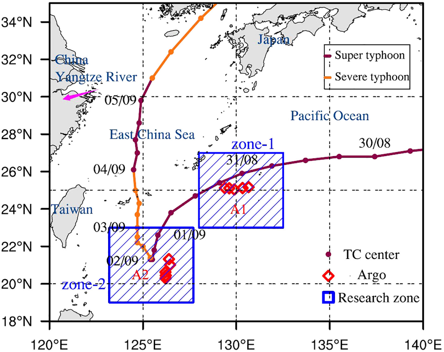
Figure 1 Research zones and Argo positions along the track of the tropical cyclone Hinnamnor (2022). The times at 0000 UTC from August 30 to September 5 are labeled.

Kashem et al. (2019) defined the ILD as the depth where the temperature is one degree lower than that of the ocean at 5 m depth, and the BLT was estimated by subtracting the ILD and MLD. The MLD was evaluated based on the density criteria of Kara et al. (2000). The formulation of the criteria was defined as following Equation (1):

$\begin{array}{ll}\text{Δ}{\text{σ}}_t={\sigma }_t(T+\text{Δ}T, S,p)-{\sigma }_t(T, S,p),& (1)\end{array}$

where T, S, and p represent the temperature, salinity, and pressure, respectively, of the sea surface around the Argo floats. Here, the temperature and salinity at 3 m depth Argo profiles were considered the SST and SSS values, and the surface pressure was considered zero. The vertical eddy viscosity in the upper ocean was estimated by the K-profile parameterization (KPP) scheme, which was formulated as Equation (2) (Large et al., 1994; McWilliams et al., 2012; Song and Xu, 2013):

$\begin{array}{ll}\text{EV}(z)=-{\text{c}}_1{\text{u}}_{*} z{(1+z/\text{h})}^{\mathrm{2,}}& (2)\end{array}$

where c₁ is a constant taken as 0.4; u_* is the oceanic friction velocity obtained from the ERA5 reanalysis data; z axis is along the vertical direction with a positive direction upward, and still water level is z = 0; and h is the depth of the boundary layer depth. The normalized depth -z/h increased from 0 at the sea surface to 1 at the bottom of the boundary layer, and the depth h was adopted at 200 m in this study.

3 Results and analyses

3.1 Synopsis of STY Hinnamnor (2022)

Hinnamnor initially originated as a tropical depression on the afternoon of August 28, 2022, in the Northwest Pacific (Figure 1). It moved westward and quickly intensified into a super typhoon at 1800 UTC on August 29 near the location 27°N, 139°E. After the replacement of the eye wall from August 30 to September 1, it began to move northward and weakened into a severe typhoon on September 2. On September 4, under the influence of the high surface temperature in the East China Sea, Hinnamnor (2022) absorbed more energy from the upper ocean and then reached the super level again. This situation persisted for one more day along its northward movement and was downgraded to a severe typhoon at 0600 UTC on September 5. After one day, the tropical storm finally landed on Geojedo Island in the south of the Republic of Korea.

3.2 Variations in the oceanic parameters from Argo data

Along the track of Hinnamnor (2022), two Argo profiling floats were selected with the following requirements. The location of the Argo float had to be within a vicinity of 200 km from the typhoon center and the observational profiles at pre-, during, and post-STY had to be captured. Since the life cycle of Hinnamnor was from August 28, 2022, to September 6, 2022, the pre- and post-STY periods were defined as the days before August 28 and after September 6, respectively. The temporal resolution of the Argo floats was one day. Their trajectories from August 21 to September 12 are illustrated in Figure 1. Table 1 lists the selected Argo ID numbers and the six estimated oceanic parameters [SST, SSS, ILD, BLT, MLD, EV (at 60 m)].

Table 1

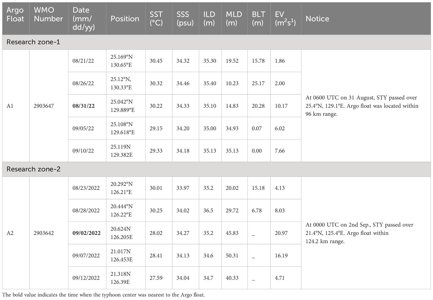
Table 1 Information on Argo floats and estimated oceanic parameters in the research zones.

The Argo profiles in zone-1 (23°N–27°N, 128°E–132.5°E) were analyzed to explore the vertical profiles along STY Hinnamnor (2022). The STY passed zone-1 from 1800 UTC on August 30 to 1200 UTC on August 31, and the first Argo float (Argo ID 2903647) was active in this zone. At 0600 UTC on August 31, the position of the center of Hinnamnor (2022) was located (25.4°N, 129.1°E). At this time, the first Argo float was situated on the left-hand side of the typhoon and nearest to the center, at approximately 96 km. Before the STY passed zone-1, where the first Argo float was located (August 26, 2022), the SST and SSS were high, and their values were 30.32 °C and 34.46 psu, respectively. The depths of the ILD, MLD, and BLT were 35.40 m, 10.23 m, and 25.17 m, respectively. In this situation, the depth of the BLT was more than one time deeper than the MLD. The value of EV was 2.00 m² s⁻¹, which indicated a slight turbulence mixing. After the STY passed zone-1 (September 05, 2022), the SST and SSS were 29.15 °C and 34.20 psu, respectively. The SSS and SST decreased by 1.17 °C and 0.26 psu, respectively, because of strong winds or heavy precipitation. The MLD increased up to 34.93 m. Figures 2C, D demonstrate that the MLD deepened because of Hinnamnor (2022). The ILD exhibited only a slight change, which was up to 35.00 m. The BLT and EV were 0.07 m and 6.02 m² s⁻¹, respectively. The BLT was comparatively less than that pre-STY, whereas the EV was in reverse, which indicates that turbulence mixing was enhanced by STY Hinnamnor (2022). The variations of the six oceanic parameters measured by Argo 1 are illustrated in Figure 2.

Figure 2

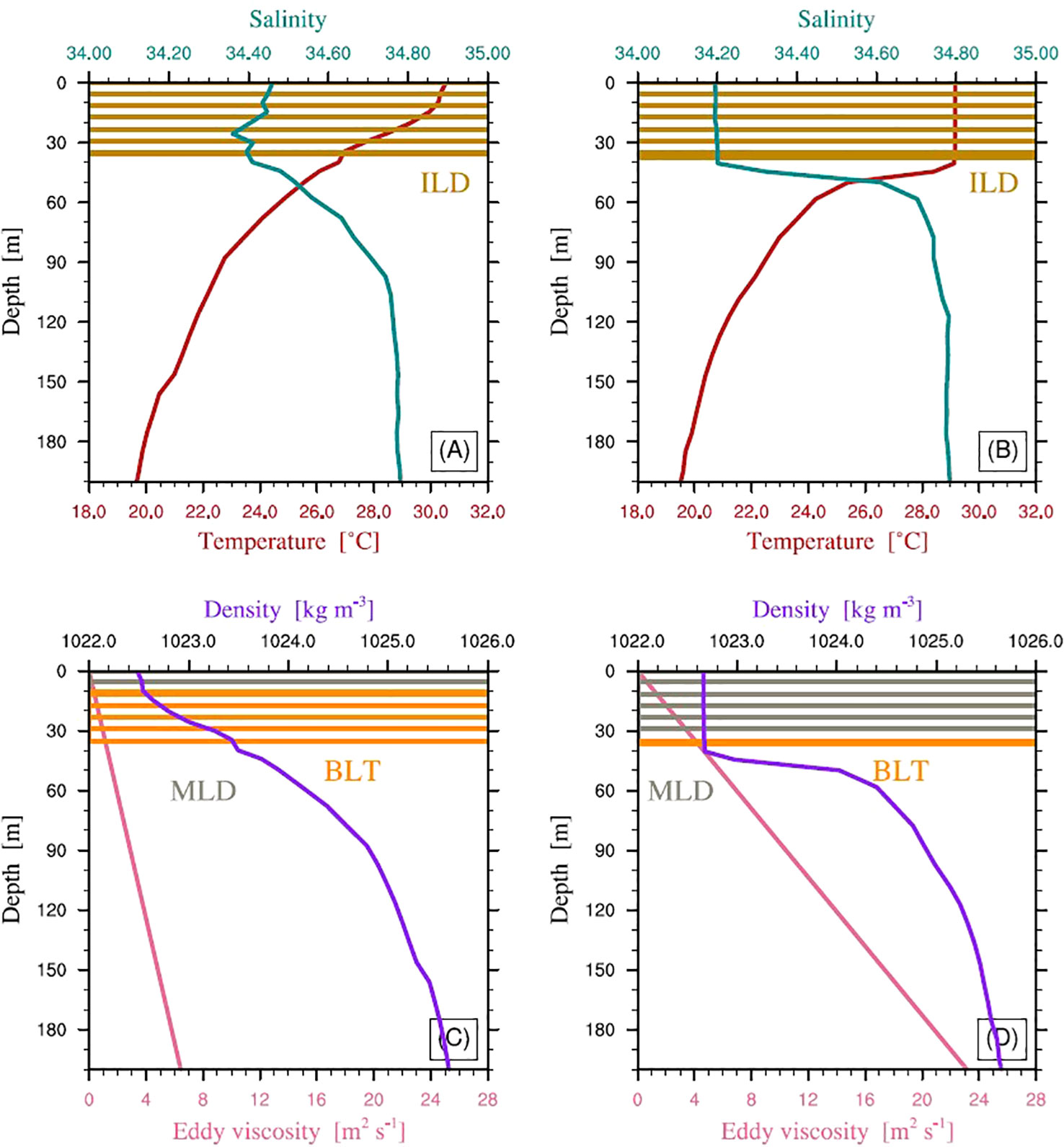
Figure 2 The vertical profiles of ocean temperature (red solid lines), salinity (green solid lines), density (purple solid lines), and eddy viscosity (pink solid lines) at Argo 1. Subplots (A, C) illustrate profiles at pre-STY (August 26, 2022) and subplots (B, D) illustrate post-STY profiles (September 05, 2022). The brown solid lines in subplots A and B denote the area where the IDL is located. The grey and orange lines in subplots C and D denote the area where the MLD and the BLT are located.

Research zone-2 was chosen within 19°N–23°N and 123.2°E–127.2°E. From 0000 UTC on September 1 to 0000 UTC on September 3, STY Hinnamnor (2022) passed this area, and the second Argo (Argo ID 2903642) was active near the track. A comparatively more dramatic variation occurred in the upper ocean because of the long stay time of the typhoon center in zone-2. At 0000 UTC on September 2, the position of the center of Hinnamnor (2022) was located at 21.4°N, 125.4°E. At this time, the second Argo float was situated at the left-hand side of the track and nearest to the typhoon center, at approximately 124.2 km. After the STY passed zone-1 where the second float was located (September 07, 2022), the SST decreased from 30.25 °C to 28.41 °C, the MLD deepened from 29.72 m to 50.31 m, the EV enhanced from 8.03 to 16.19 m² s⁻¹, and the BLT disappeared. The SSS was 34.02 psu before the STY passed the Argo and then increased to 34.13 psu after the STY passed the float, which is a reverse variation compared to zone-1. This increment of SSS in zone-2 indicates the impact of vertical mixing or subsurface upwelling on the distribution of oceanic salinity, which is more significant than precipitation. The BLT in zone-2 disappeared earlier. The vertical profiles of water temperature and salinity from the two Argo floats, before and after the passing of the STY, are illustrated in Figure 3. It also illustrates the changes in salinity near the ocean surface when the STY passed the two zones. This reveals that the typhoon-induced vertical turbulent mixing or upwelling in zone-2 was more intensive than that in zone-1. These physical processes carried high salinity water at the deep level up to the sea surface, which increased the SSS (D’Asaro et al., 2007; Cheung et al., 2013).

Figure 3

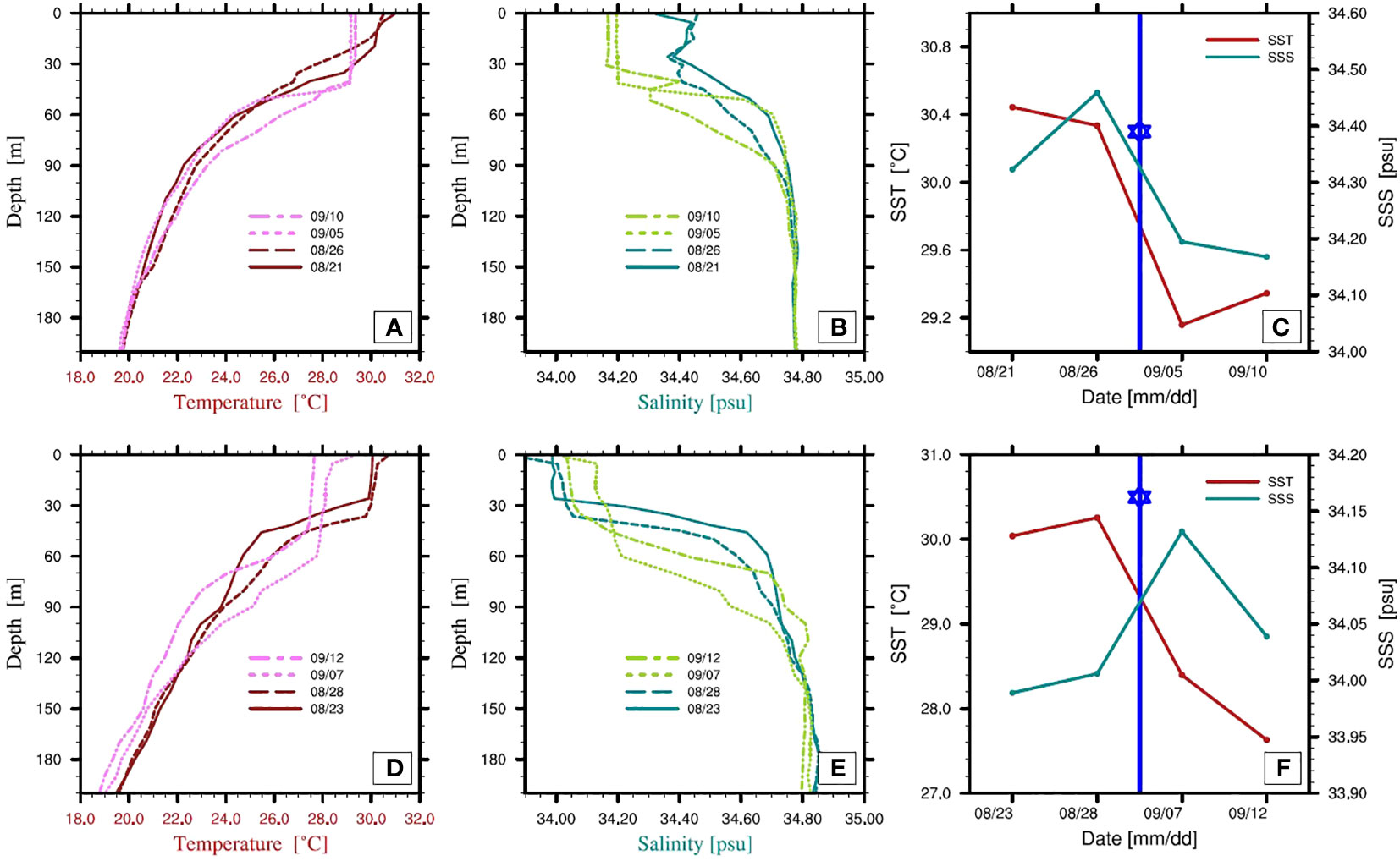
Figure 3 The vertical profiles of ocean temperature and salinity along STY Hinnamnor at Argo 1 (A, B) and Argo 2 (D, E). The variation of SST and SSS at Argo 1 (C) and Argo 2 (F). The blue solid lines with a star symbol present the arrival time of the cyclone center.

3.3 SST cooling due to STY Hinnamnor (2022)

Here, the microwave optimally interpolated the SST data provided by the remote sensing system, which was used to study the SST evolution during the passage of Hinnamnor (2022) from August 26 to September 6. The spatial and temporal resolutions of the dataset are 0.25° and one day, respectively. The satellite-observed SSTs at six moments are presented in Figure 4. Previous studies have proposed that strong winds and a deepened mixed layer could result in SST cooling by several degrees along the typhoon track (Cheung et al., 2013; Kashem et al., 2019). Figure 4 illustrates the SST distribution during the passage of STY Hinnamnor (2022). On August 26, 2022, the SST of the majority of the Pacific within 18°N–27°N and 123°E–140°E was above 30.0 °C, and the SST near 135°E was even above 30.8 °C. The typhoon center entered this region at 1800 UTC on August 29, and the decrease of SST appeared along the track on September 1 (Figure 3B). On September 2, 2022, the STY switched its direction of movement from southwest to north. A day after, the SST in the majority of the region (20°N–25°N,123°E–127°E) was below 30.0 °C because of strong winds and enhanced MLD. The SST even dropped below 27.0 °C in the vicinities of the locations in which typhoon centers passed. On September 5, the reduction of SST further extended northward along the track of Hinnamnor (2022) because the typhoon intensified into the super level again on September 4. Similarly, strong winds and deepened MLD associated with the STY played a crucial role in SST reduction. The STY hit Geojedo Island in the south of the Republic of Korea on September 6, 2022, and the SST in a part of the area along the track of Hinnamnor (2022) slightly increased to the pre-STY status. The SST pattern in Figure 4 denotes that the maximum SST reduction was more prominent in zone-2 than in zone-1, and the greatest decrease was approximately 3 °C. The long duration of typhoon centers in zone-2 intensified the turbulent mixing so that more cold water was carried upward to the sea surface. The maximum depth of the mixed layer in zone-2 was nearly 60 m post-STY, whereas it was only 40 m in zone-1 (refer to Figures 3A, D).

Figure 4

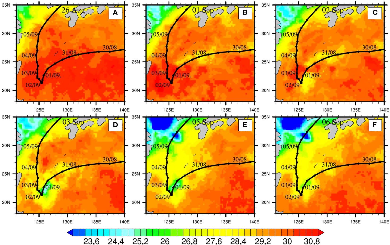
Figure 4 The evolution of SST because of STY Hinnamnor (2022). The time at 0000 UTC from August 30 to September 5 is labeled. The evolution of SST because of STY Hinnamnor (2022). The time at 0000 UTC on 26 Aug (A), 1st Sep (B), 2nd Sep (C), 3rd Sep (D), 5 Sep (E), and 6 Sep (F).

3.4 Comparison of the ocean temperature and salinity between pre- and post-STY

The HYCOM reanalysis data from the Global Ocean Forecasting System 3.1 (GOFS 3.1) are used in Figure 5 to demonstrate the vertical profiles of ocean temperature and salinity pre- and post-STY along the track of Hinnamnor (2022). The reanalysis data used in this study have a spatial resolution of 0.08°lon × 0.04°lat and a temporal interval of one day. Here, the data collected were along the latitude averaging 18°N–30°N. The vertical profiles of temperature along the longitude (123°E–140°E) are presented in subplots A and B in Figure 5. Pre-STY (Figure 5A) demonstrates that the SST was above 30.0 °C, and the depth with water temperature above 30.0 °C was as deep as 20 m near the longitude 125°E. High SSTs signify the potential for the formation of tropical cyclones in the Northwest Pacific. Post-STY (Figure 5B) denotes that the SST was reduced due to the vertical mixing and heavy upwelling associated with tropical cyclone Hinnamnor (2022). The SST was below 28 °C in the vicinities of 126°E longitude. In this area, the upwelling rushed up and mixed with the subsurface layer; hence, the BLT became shallower and then disappeared.

Figure 5

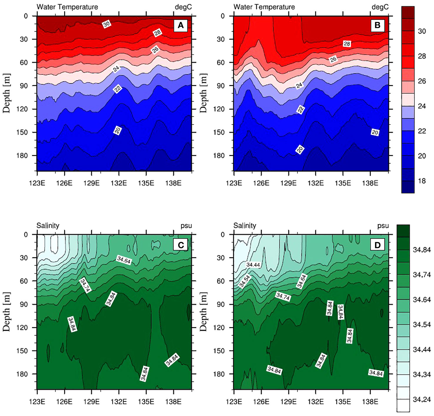
Figure 5 The vertical profiles (123°E –140°E) of temperature and salinity in the ocean from August 26, 2022 (i.e., pre-STY) in subplots (A, C) to September 06, 2022 (i.e., post-STY) in subplots (B, D) along the track of STY Hinnamnor (2022).

The subplots C and D in Figure 5 present the pre-STY and post-STY vertical salinity profiles of the ocean along the track of STY Hinnamnor (2022). Pre-STY (Figure 5C) demonstrates that the SSS was approximately 34.64 psu near the longitude 132°E and below 34.44 psu near the longitude 125°E. Below the sea surface, salinity stratifications were much weaker within 30 m in both regions. This inhibition of vertical mixing is caused by the freshwater input from continental rivers, such as the Yangtze River in China. Based on the ECMWF HROF re-analysis dataset, Figures 6A–C classifies the daily runoff distribution at three typical dates. The runoff on August 26 could prove this view, which is also consistent with the previous insight that the SSS was significantly affected by freshwater input (Sprintall and Tomczak, 1992). The depth of the low saline area (below 34.34 psu) was almost 35 m at 123°E–128°E, as demonstrated in Figure 5C. Interestingly, Figure 5A illustrates that the water temperature in the top 35 m was warmer in this region. The low SSS at the top of the upper ocean effectively sustained the warm water temperature because of the little vertical mixing. Net heat was trapped within the thin oceanic stratified layer because of the freshwater input. Post-STY (given in Figure 5D), heavy precipitation caused the decrease of SSS from 34.6 psu to 34.5 psu at 129°E–135°E. The distribution of precipitation is presented in Figure 7 in accordance with the satellite data. Within this region, the accumulated results of precipitation and runoff were approximately 15728.72 mm and 753.91 mm, respectively, during the period of Hinnamnor (2022). However, there was no evident variation of SSS at 123°E–128°E pre- and post-STY. The dramatic reduction of SST (Figure 4) reveals that strong vertical mixing occurred in the area within 18°N–30°N and 123°E–128°E. The convex isotherm in Figure 5B indicates that induced upwelling also appeared in this region because of STY Hinnamnor (2022). The combined effects of these two physical processes should have increased the SSS, but that did not happen. The accumulated precipitation and runoff in Figures 6, 7 imply that freshwater input decreased the SSS in this region. The accumulated precipitation and runoff were approximately 50176.58 mm and 4111.71 mm, respectively, from August 26 to September 6. The saline profile in the western region (123°E–128°E) also denotes that the upwelling impact on salinity was absent at 60 m deep, as demonstrated in Figure 5D. This result shows that freshwater from runoff and precipitation diluted the near-surface dense saline water that was brought to the subsurface ocean by upwelling from the deep ocean.

Figure 6

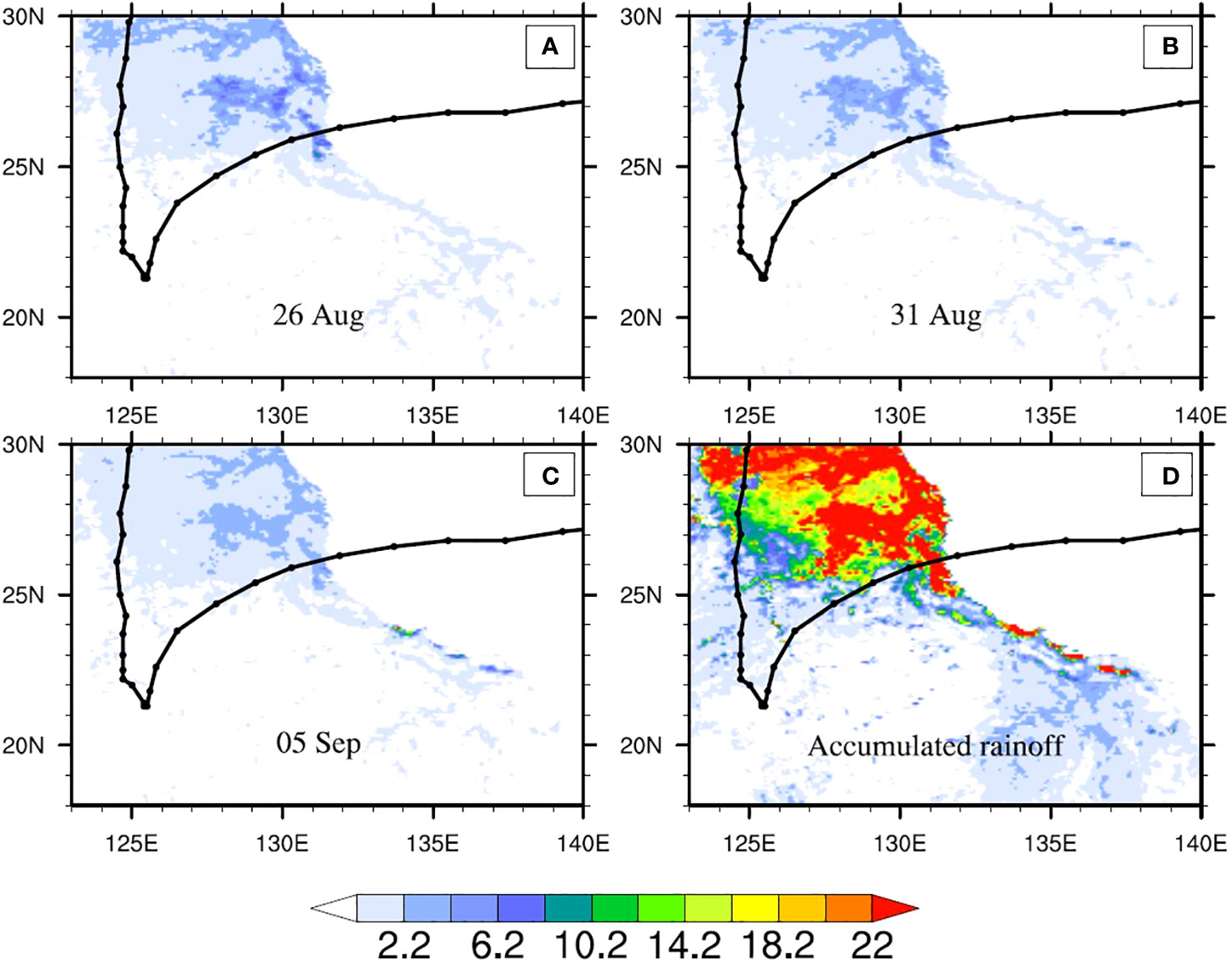
Figure 6 The evolution of daily runoff (units: mm) because of STY Hinnamnor (2022). Three typical times from August 26 to September 6 are labeled in subplots (A–C). Subplot (D) denotes the accumulated runoff from August 26 to September 6.

Figure 7

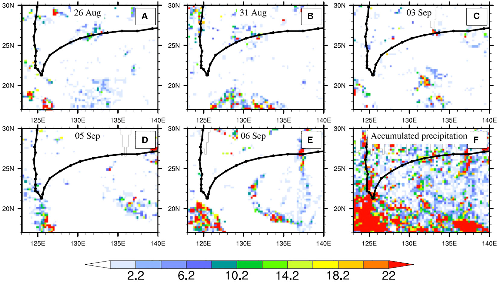
Figure 7 The evolution of daily precipitation (units: mm) because of STY Hinnamnor (2022). Five typical times from August 26 to September 6 are labeled in subplots (A–E). Subplot (F). denotes the accumulated precipitation from August 26 to September 6.

3.5 Variations in air–sea heat fluxes and upper ocean heat budget during Hinnamnor (2022)

Based on the European Center for Medium-Range Weather Forecasts (ECMWF) ERA5 re-analysis hourly data, Table 2 classifies the daily averaged fluxes of net shortwave radiation (NSWF), net longwave radiation (NLWF), sensible heat (SHF), latent heat (LHF), total heat loss (THL), and net surface heat flux (NHF) in the region (18°N–35°N, 120°E–140°E) along the track of STY Hinnamnor (2022) from August 26 to September 6. The THL was estimated by adding the LHF, SHF, and NLWF. The NHF was estimated by the sum of NSWF and THL. The sky above this region was covered with higher cloudiness, and the speed of the near-surface airflow was stronger starting from August 30, 2022, under the influence of the tropical cyclone. As a result, the NSWF reduced, and the LHF, which is denoted as negative to present the heat loss component, increased. The NHF exhibited a decreasing trend until September 6 and became a negative value, signifying increasing heat loss from the sea surface to the atmosphere during the passage of STY Hinnamnor (2022). The NSWF exhibited the minimum value (148.11 W m⁻²) on September 3 and slightly increased on September 4. The LHF exhibited the maximum value (−217.11 W m⁻²) on September 3, which indicates the largest latent heat loss. On the same day, the largest NHF decrease reached 124.79 W m⁻². The re-analysis data provide reliable evidence for the behavior of the surface fluxes pre-, during, and post-STY Hinnamnor (2022).

Table 2

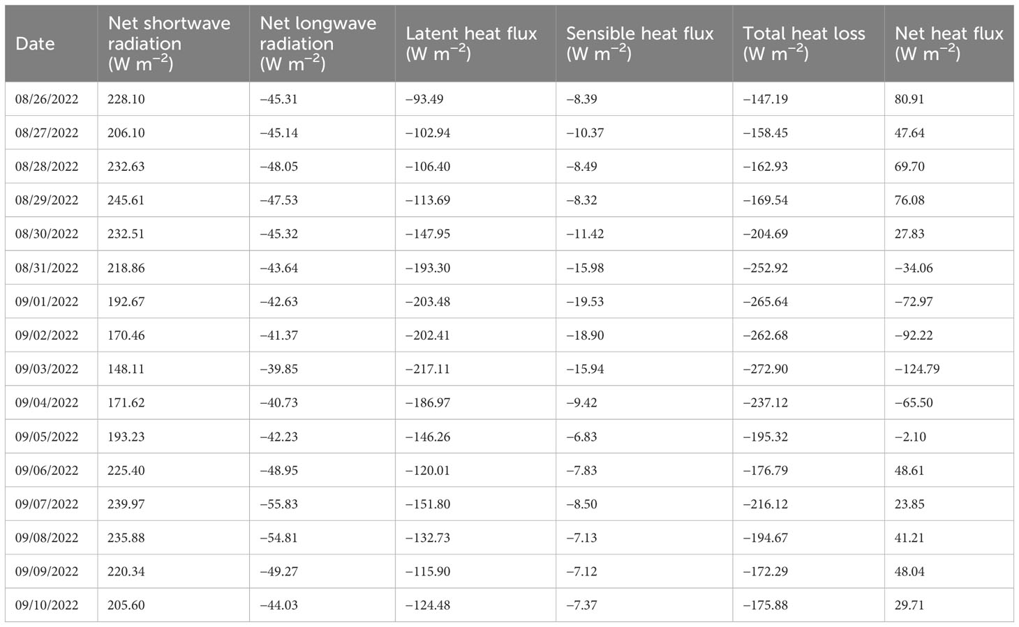
Table 2 Based on the ERA5 re-analysis data, the heat budget of the upper ocean of the region (18°N–35°N, 123°E–140°E) along the track of Hinnamnor (2022).

Figure 8 presents the time series of the six fluxes in the cyclone track domain (18–35°N, 120–140°E). The ERA5 re-analysis data with low spatial resolution usually underestimates the TC intensity. The results obtained from the ECMWF high-resolution operational forecast (HROF) data with 0.08 degrees are also illustrated in Figure 8 for comparison. They denote that the daily maximum NSWF was lower from August 31 to September 5 than the previous and following days because of the strong winds and high cloudiness associated with Hinnamnor (2022). The variation of the daily maximum NSWF exhibited a symmetric pattern during this period: it first decreased to a minimum around September 4 and then increased. The mean LHF kept increasing from August 30 to September 4. Large quantities of water vapor (evaporation) formed condensation clouds in the sky, and high cloudiness decreased the NSWF during this period. The NSWF slightly returned to the pre-STY status on September 6, 2022, owing to the weakening of the tropical cyclone and the landfall on Geojedo Island in the Republic of Korea. The overall behavior of the maximum NSWF obtained from the HROF data from August 26 to 31 was prominently greater than 800 W m⁻² because of its high resolution. Its time series also indicated the presence of dense cloudiness in the sky during Hinnamnor (2022).

Figure 8

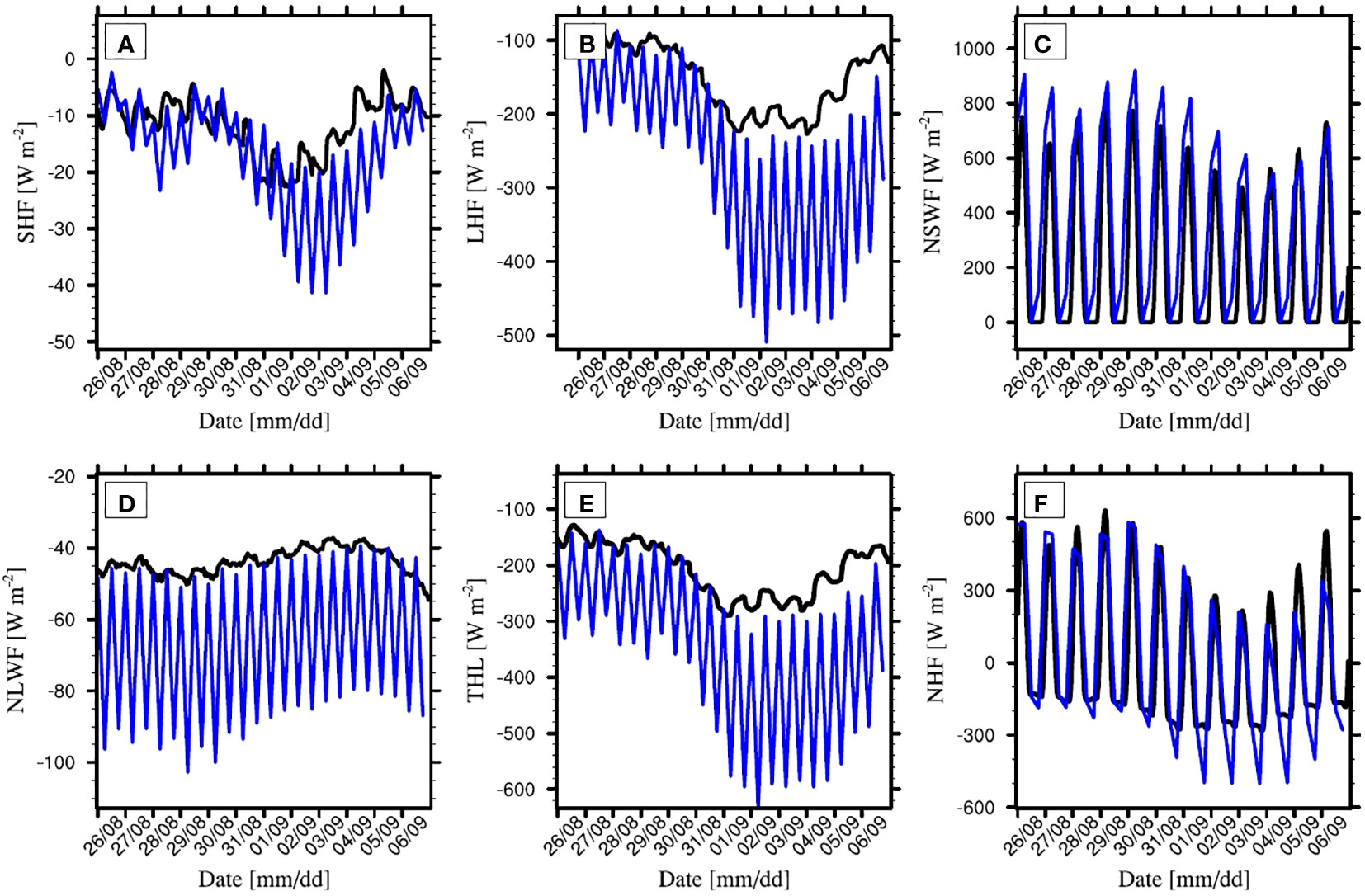
Figure 8 Time series of (A) SHF, (B) LHF, (C) NSWF, (D) NLWF, (E) THL, and (F) NHF during the passage of Hinnamnor (2022). The black and blue lines denote the re-analysis data from the ECMWF ERA5 and HROF, respectively.

The mean LHF during August 26–30 was less than that from August 31 to September 5. The LHF dramatically increased to 200 W m^-2 after August 30 and reached the maximum of around 0000 UTC on September 4, which resulted in the formation of condensation clouds from water evaporation. This could explain the low NSWF demonstrated in Figure 8C during this period. Compared to the SHF, the LHF controlled the total heat loss from the ocean (refer to Figure 8E) and promoted further development of the tropical cyclone. The high LHF also caused a considerable decrease in the net heat flux (refer Figure 8F). On the morning of September 4, Hinnamnor (2022) intensified to the super level once again and continued moving northward. At this moment, the STY with moist airflow contained higher humidity than the previous one that formed on August 30. The LHF is proportional to the humidity difference between the atmosphere and the sea surface airflow. Hence, the LHF gradually decreased starting from September 4 because of the small humidity difference between the sea surface and airflow. After the landfall of Hinnamnor (2022) on September 6, the LHF increased a little but tended to decrease. The mean LHF obtained from HROF was two times that of ERA5 because of the high spatial resolution (in Figure 8B). Compared to the ERA5 re-analysis data, the HROF results presented a more dramatic increment of LHF from August 31 to September 4.

The variation of the SHF and the LHF has a similar pattern. The SHF presented a dramatic reduction from August 31 to September 4 because of the presence of strong winds and heavy precipitation. After September 4, the SHF decreased owing to the small temperature difference between the sea surface and the atmosphere. Lin et al. (2008) considered that SST cooling and the high temperature of the airflow over the sea surface restrained the air–sea sensible heat exchange. This view can also be used to interpret the decrease in mean SHF after September 4, which is given in Figure 8D. The high-resolution HROF data reveal greater SHF during the whole period, especially from August 31 to September 4, which was nearly twice the results from the ERA5 re-analysis data. The variations of the SHF (Figure 8A) and the LHF (Figure 8B) reveal a dynamic thermal equilibrium between the atmosphere and ocean during the passage of the STY. Initially, the tropical cyclone developed by absorbing heat from the ocean. The turbulent fluxes, which include the SHF and the LHF, played an important role in cyclone intensification. The magnitude of the SHF and the LHF increased continuously to lose the ocean heat. When the typhoon intensified into the STY, the energetic cyclone system with high temperature and humidity inhibited heat transport from the ocean to the atmosphere. The northward movement of STY Hinnamnor (2022) from September 4 to 6 stopped the incremental transfer of heat from the ocean to the atmosphere.

Both the ERA5 and HROF re-analysis data reveal that the NHF arrived at the lowest point from August 31 to September 4, as demonstrated in Figure 8F. Correspondingly, the greatest THL and the lowest NSWF occurred during this time (Figures 8E, C). The high heat losses and small heat acquisition point to the significant impact of STY on the heat budget of the research domain. The re-analysis data show that the magnitude of mean NLWF began to decrease on August 31 and reached the minimum on September 4 (Figure 8D). Following this, the mean NLWF began to increase.

3.6 Anomalies of the parameters of surface waves due to STY Hinnamnor (2022)

The ERA5 re-analysis data during the passage of STY Hinnamnor (2022) were used to investigate the anomalies of surface waves. The evolution of the mean significant wave height (SWH), mean wave period (MWP), and spectral peak period (SPP) is depicted in Figures 9, 10. On August 26, the mean SWH was below 2 m and uniformly distributed in the research domain within 18°N–35°N and 120°E–140°E (Figure 9A). At this moment, the MWP decreased from the east to the west: the maximum was approximately 9 s in the east and the minimum below 5 s in the west (Figure 9E). In the East China Sea (23°N–32°N, 117°E–131°E), the MWP in the middle was nearly 4 s lower than that in the north and south sides. On August 31, STY Hinnamnor (2022) entered the East China Sea from the east. The distributions of the SWH and the MWP are presented in Figures 9B, F. The maximum SWH over 7 m emerged on the right-hand side of the cyclone track, and the maximum MWP exceeding 9 s appeared on both sides of the track. The main reason for SWH spatial variation is that surface waves on the right side of the cyclone center obtained more momentum from strong surface winds. Large values of the MWP near the cyclone center imply the generation of swell driven by the STY, which was in accordance with the numerical study of Xu et al. (2017). Figure 9F also indicates that the MWP in the east of the research domain decreased by ~2–3 s compared with Figure 9E. This signifies the generation of wind waves in this region (134°E–140°E) after Hinnamnor (2022) passed.

Figure 9

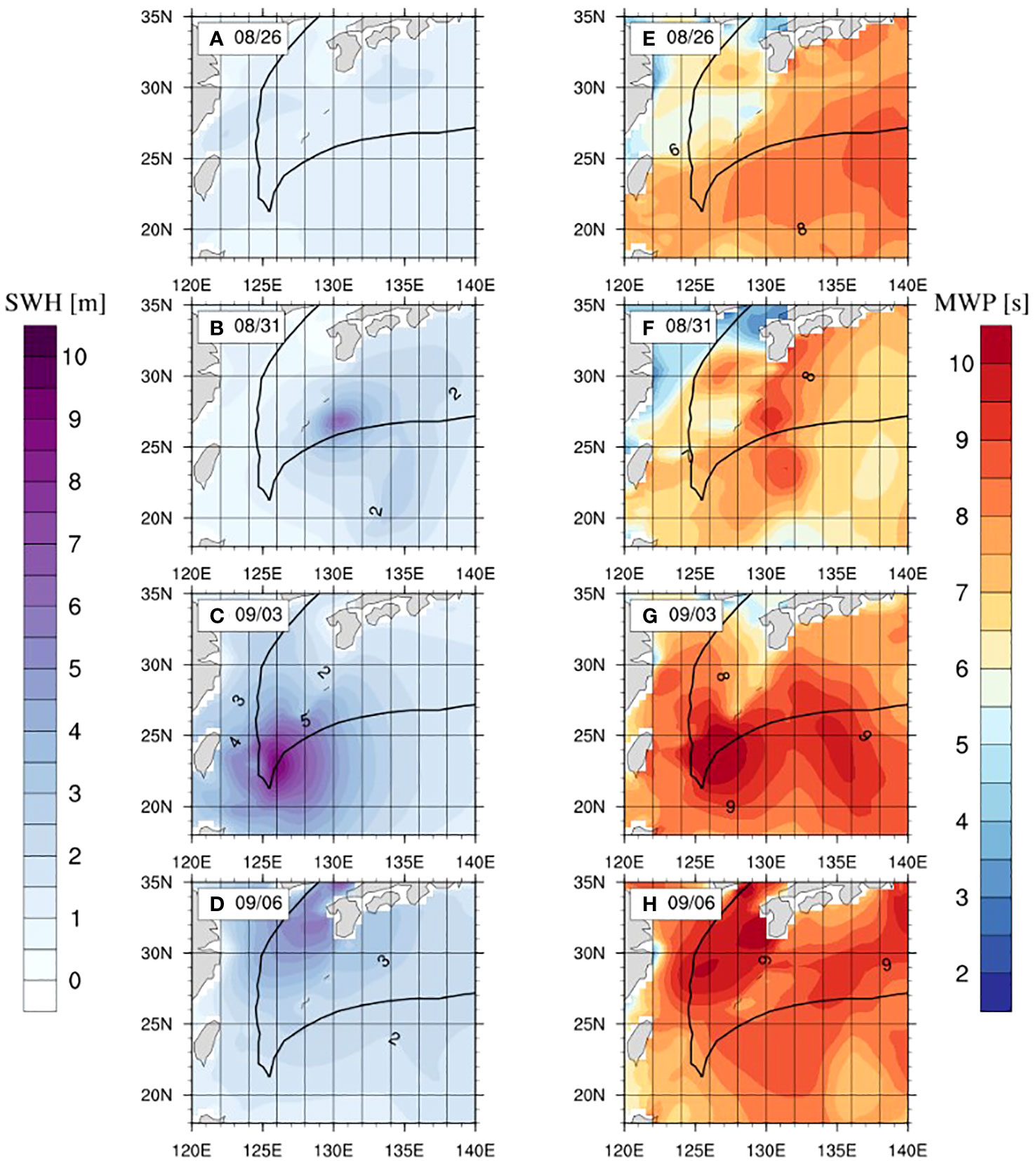
Figure 9 Anomalies of SWH (A-D) and MWP (E-H) at 0000 UTC on August 26, August 31, September 03, and September 06. Black lines denote the STY track.

Figure 10

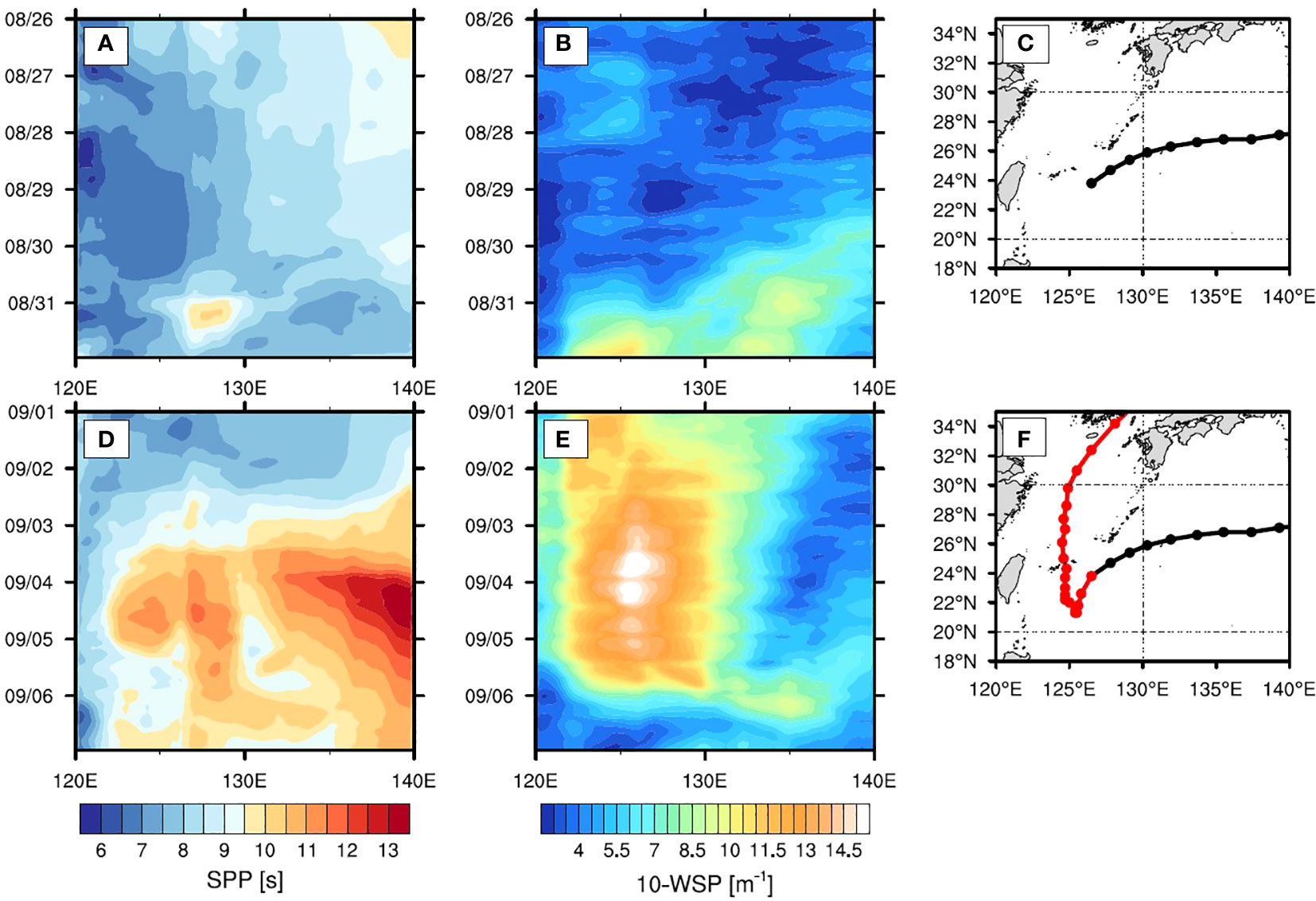
Figure 10 The temporal evolution of SPP (in subplot A) and 10-WSP (in subplot B) along the longitude during August 26–31 (track in subplot C); the temporal evolution of SPP (in subplot D) and 10-WSP (in subplot E) along the longitude during September 1–6 (track in subplot F).

On September 3, the typhoon center moved northward with a maximum wind speed of approximately 42 m s⁻¹. The spatial distributions of the SWH and the MWP are summarized in Figures 9C, G. At this time, the maximum SWH increased to 10 m and positioned where the typhoon began to switch its direction of movement. Compared with Figure 9B, the region with SWH higher than 5 m was also further enlarged along the track of Hinnamnor (2022) because of the prolonged impact of strong winds on this sea area (20°N–25°N, 125°E–128°E). In addition, prolonged strong winds prominently increased the whole MWP of the research domain (Figure 9G). The maximum MWP also appeared on both sides of the typhoon center and reached above 10 s. In the area far away from the typhoon track, the MWP was generally as low as 6–7 s. Figure 9G also denotes that the MWP in the south of the track was 1–2 s greater than that in the north. This is attributed to the movement of the direction of the cyclone center before September 3. Hinnamnor (2022) kept moving southwest from August 29 and generated more swell in the south. On the morning of September 6, Hinnamnor (2022) landed, and no strong winds influenced the research domain. The SWH returned to a small value except for the area near the location where the typhoon landed (Figure 9D). At this time, the MWP increased in the north because the swell in the south propagated northward (Figure 9G). The anomaly of the SWH during the four typical moments reveals that the wave heights were associated with wind speeds, and its largest value occurred on the right side of the cyclone center. A massive swell was generated near the cyclone center when large MWPs emerged on both sides of the center. Along with the movement of the STY, the swell widely propagated northward after September 3.

Figure 10 illustrates how the SPP varied with time and longitude in the research domain. This can be used to further study the effect of Hinnamnor (2022) on the wave period. Correspondingly, the temporal and spatial evolution of the wind speed at 10 m above the sea surface (10-WSP) is also presented in Figure 10. Latitude averaging for the SPP and 10-WSP was conducted over the entire 18°N–33°N domain. Figure 10C presents the tropical cyclone track at 0000 UTC from August 29 to 1800 UTC on August 30. In the pre-STY status (during August 26–27), the averaged SPP was lower than 9 s (Figure 10A), and the mean 10-WSP was lower than 5 m s⁻¹ (Figure 10B). On August 31, when the 10-WSP increased to 8 m s⁻¹ near 130°E, the SPP slightly increased from 126°E to 130°E (Figure 10A). Before Hinnamnor (2022) intensified into an STY for the second time (during September 1–3), the 10-WSP within 123°E–128°E continued to enhance, whereas the SPP had little increment. This indicates the domination of wind waves over wave energy within this longitude range. After the northward movement, Hinnamnor (2022) developed into an STY on September 4 (Figure 10F), and the 10-m WSP within 123°E–127°E sustained above 10 m s⁻¹ until September 6. In this region, the SPP increased to greater than 10 s during September 4–5 and then decreased to less than 10 s from September 5. The eastern region (133°E–140°E) demonstrated a significant SPP increase where the 10-m wind speed was lower than 5 m s⁻¹. Swell appearance in this region is considered to be the result of the eastward propagation of wind waves near the cyclone center.

4 Conclusion and discussion

Every year, dozens of typhoons form and traverse the Northwest Pacific. The complicated mechanisms of typhoon formation and evolution demand continuous exploration. This study considered STY Hinnamnor that occurred in 2022 as an example to investigate the features of the upper ocean responses and surface waves during a typhoon. Argo (in situ) observations together with the satellite, meteorological, and oceanic re-analysis results were used to reveal the temporal and spatial variations of the upper ocean. Potential reasons for the formation of the phenomena associated with air–sea interactions were also discussed. The research is summarized as follows:

(1) At the location where the STY passed southwestward (zone−1), the Argo profiles revealed that the post-STY SST, SSS, ILD, and BLT decreased by 1.17 °C, 0.26 psu, 0.4 m, and 25.1 m to pre-STY, respectively, whereas the post-STY MLD and EV increased by 24.7 m and 4.02 m² s⁻¹ to pre-STY, respectively. At the location where the STY began to move northward (zone-2), the Argo profiles revealed that the post-STY SST, ILD, and BLT decreased by 1.84 °C, 0.4 m, and 6.78 m to pre-STY, respectively, whereas the post-STY SSS, MLD, and EV increased by 0.11 psu, 20.59 m, and 8.16 m² s⁻¹ to pre-STY, respectively. The Argo data revealed that the reduction of SST and ILD and the increment of MLD and EV in zone-2 were two times greater than those in zone-1. This implies that the vertical mixing or the upwelling—which brought cold water upward to the mixed layer—that occurred in zone-2 was more intensive. The SSS in zone-1 decreased because the freshwater (i.e., precipitation or runoff) input suppressed its increase.

(2) The remote sensing data provided the evolution of SST during the STY. The SST near the cyclone track significantly decreased and presented a more dramatic decrease in zone-2 than in zone-1. The longer strong winds and deeper MLD in zone-2 were the main reasons for this phenomenon.

(3) The HYCOM reanalysis data were used for latitude averaging of the ocean temperature and salinity within the region where the STY passed. The vertical profiles of ocean temperature revealed a strong upwelling near the 126°E longitude post-STY. The typhoon center moved northward in the vicinities of the 126°E longitude from 0000 UTC on September 2 to 1200 UTC on September 5. Hence, persistent strong winds in this region led to the formation of upwelling. However, in the region within 123°E–128°E, the vertical profiles of ocean salinity near the sea surface had little change between the pre- and post-STY conditions. The freshwater input in this region significantly inhibited the increase in near-surface salinity. One source of freshwater was the runoff, mainly contributed by the Yangtze River in China. From August 26 to September 6, the accumulated precipitation of the runoff in the 18°N–35°N and 123°E–128°E domains was approximately 50176.58 mm. The other source of the freshwater input was heavy precipitation, and its accumulated results reached approximately 4111.71 mm during the period of Hinnamnor (2022).

(4) The time series of the six fluxes within the research region was investigated based on the ECMWF ERA5 and HROF re-analysis datasets. The LHF began to decrease from August 31 and reached the maximum around September 4. The increment of LHF resulted in the formation of condensation clouds from water evaporation. High cloudiness in the sky made the NSWF reach its lowest point during this period. Compared with the SHF, the LHF dominated the total heat loss from the ocean to the atmosphere and promoted further development of the tropical cyclone. In addition, the variations of the SHF and LHF indicate a dynamic thermal equilibrium during the passage of the STY. Initially, the tropical cyclone developed by absorbing heat from the ocean. The SHF and LHF quickly increased to intensify the tropical cyclone. When the typhoon intensified to the super level, the cyclone system with high temperature and humidity inhibited heat transport from the ocean to the atmosphere. At this time, both the SHF and LHF began to decrease.

(5) The ECMWF ERA5 re-analysis data were used to study the anomalies of mean SWH, MWP, and SPP. Evolutions of the SWH and MWP distributions at four typical moments demonstrate the crucial impact of the STY on the surface waves. Strong winds increased the SWH from 2 m to nearly 10 m, and the maximum SWH was located on the right side of the typhoon center. The emergence of large MWPs on both sides of the cyclone center indicates the massive generation of swell. After September 3, the swell propagated northward along with the movement of the typhoon center. In the 123°E–128°E domain, the variation of the latitude averaging SSP with time indicates that the SPP had little increment before the typhoon upgraded to the super level for the second time (September 4). During September 4–6, an obvious swell region appeared in the region within 133°E–140°E, where the 10-m wind speed was lower than 5 m s⁻¹. The eastward propagation of wind waves near the cyclone center is speculated to have resulted in the appearance of the swell.

Data availability statement

The original contributions presented in the study are included in the article/Supplementary Material. Further inquiries can be directed to the corresponding author.

Author contributions

TZ: Conceptualization, Data curation, Formal Analysis, Funding acquisition, Investigation, Methodology, Project administration, Resources, Software, Supervision, Validation, Visualization, Writing – original draft, Writing – review & editing.

Funding

The author(s) declare financial support was received for the research, authorship, and/or publication of this article. This work was supported by the Project of the Education Department of Fujian Province, grant number JAT220232, and the Research Setup Funding of Fujian University of Technology, grant number GY-Z202208.

Acknowledgments

Thanks go to the colleagues in my research group for the grammar check of this manuscript.

Conflict of interest

The author declares that the research was conducted in the absence of any commercial or financial relationships that could be construed as a potential conflict of interest.

Publisher’s note

All claims expressed in this article are solely those of the authors and do not necessarily represent those of their affiliated organizations, or those of the publisher, the editors and the reviewers. Any product that may be evaluated in this article, or claim that may be made by its manufacturer, is not guaranteed or endorsed by the publisher.

References

Balaguru K., Chang P., Saravanan R., Leung L. R., Xu Z., Li M., et al. (2012). Ocean barrier layers’ effect on tropical cyclone intensification. Proc. Natl. Acad. Sci. U. S. A. 109, 14343–14347. doi: 10.1073/pnas.1201364109

PubMed Abstract | CrossRef Full Text | Google Scholar

Bender M. A., Ginis I., Kurihara Y. (1993). Numerical simulations of tropical cyclone-ocean interaction with a high-resolution coupled model. J. Geophys. Res. 98, 23245–23263. doi: 10.1029/93JD02370

CrossRef Full Text | Google Scholar

Cheung H., Pan J., Gu Y., Wang Z. (2013). Remote-sensing observation of ocean responses to Typhoon Lupit in the northwest Pacific. Int. J. Remote Sens. 34, 1478–1491. doi: 10.1080/01431161.2012.721940

CrossRef Full Text | Google Scholar

Chiang T. L., Wu C. R., Oey L. Y. (2011). Typhoon Kai-tak: an ocean’s perfect storm. J. Phys. Oceanogr. 41, 221–233. doi: 10.1175/2010JPO4518.1

CrossRef Full Text | Google Scholar

D’Asaro E. A., Sanford T. B., Niiler P. P., Terrill E. J. (2007). Cold wake of hurricane Frances. Geophys. Res. Lett. 34, L15609. doi: 10.1029/2007GL030160

CrossRef Full Text | Google Scholar

Emanuel K. A. (2003). Tropical cyclones. Annu. Rev. Earth Planet. Sci. 31, 75–104. doi: 10.1146/annurev.earth.31.100901.141259

CrossRef Full Text | Google Scholar

Emanuel K. A. (2013). Downscaling CMIP5 climate models shows increased tropical cyclone activity over the 21st century. Proc. Natl. Acad. Sci. U. S. A. 110, 12219–12224. doi: 10.1073/pnas.1301293110

PubMed Abstract | CrossRef Full Text | Google Scholar

Emanuel K., Desautels C., Holloway C., Korty R. (2004). Environmental control of tropical cyclone intensity. J. Atmos. Sci. 61, 843–858. doi: 10.1175/1520-0469(2004)061<0843:ECOTCI>2.0.CO;2

CrossRef Full Text | Google Scholar

Guan S., Zhao W., Huthnance J., Tian J., Wang J. (2014). Observed upper ocean response to Typhoon Megi, (2010) in the northern south China sea. J. Geophys. Res. Oceans 119, 3134–3157. doi: 10.1002/2013JC009661

CrossRef Full Text | Google Scholar

He H. L., Wu Q. Y., Chen D. K., Sun J., Liang C., Jin W., et al. (2018). Effects of surface waves and sea spray on air-sea fluxes during the passage of Typhoon Hagupit. Acta Oceanol. Sin. 37, 1–7. doi: 10.1007/s13131-018-1208-2

CrossRef Full Text | Google Scholar

Hong X., Li J. (2021). A beta-advection typhoon track model and its application for typhoon hazard assessment. J. Wind Eng. Ind. Aerodyn. 208, 104439. doi: 10.1016/j.jweia.2020.104439

CrossRef Full Text | Google Scholar

Huang P., Sanford T. B., Imberger J. (2009). Heat and turbulent kinetic energy budgets for surface layer cooling induced by the passage of Hurricane Frances, (2004). J. Geophys. Res. 114, C12023. doi: 10.1029/2009JC005603

CrossRef Full Text | Google Scholar

Jacob S. D., Shay L. K., Mariano A. J., Black P. G. (2000). The 3D oceanic mixed layer response to Hurricane Gilbert. J. Phys. Oceanogr. 30, 1407–1429. doi: 10.1175/1520-0485(2000)030<1407:TOMLRT>2.0.CO;2

CrossRef Full Text | Google Scholar

Jaimes B., Shay L. K. (2009). Mixed layer cooling in mesoscale oceanic eddies during hurricanes Katrina and Rita. Mon. Weather Rev. 137, 4188–4207. doi: 10.1175/2009MWR2849.1

CrossRef Full Text | Google Scholar

Jin F. F., Boucharel J., Lin I. I. (2014). Eastern Pacific tropical cyclones intensified by el Niño delivery of subsurface ocean heat. Nature 516, 82–85. doi: 10.1038/nature13958

PubMed Abstract | CrossRef Full Text | Google Scholar

Kara A. B., Rochford P. A., Hurlburt H. E. (2000). An optimal definition for ocean mixed layer depth. J. Geophys. Res. 105, 16803–16821. doi: 10.1029/2000JC900072

CrossRef Full Text | Google Scholar

Kashem M., Ahmed M. K., Qiao F., Akhter M. A. E., Chowdhury K. M. A. (2019). The response of the upper ocean to tropical cyclone Viyaru over the Bay of Bengal. Acta Oceanol. Sin. 38, 61–70. doi: 10.1007/s13131-019-1370-1

CrossRef Full Text | Google Scholar

Large W. G., McWilliams J. C., Doney S. C. (1994). Oceanic vertical mixing: a review and a model with a nonlocal boundary layer parameterization. Rev. Geophys. 32, 363–403. doi: 10.1029/94RG01872

CrossRef Full Text | Google Scholar

Lin I. I., Wu C. C., Pun I. P., Ko D. S. (2008). Upper-ocean thermal structure and the western North Pacific Category 5 typhoons. Part I: Ocean features and the Category 5 typhoons’ intensification. Mon. Weather Rev. 136, 3288–3306. doi: 10.1175/2008MWR2277.1

CrossRef Full Text | Google Scholar

Lin S., Zhang W. Z., Shang S. P., Hong H. (2017). Ocean response to typhoons in the western North Pacific: composite results from Argo data. Deep Sea Res. I 123, 62–74. doi: 10.1016/j.dsr.2017.03.007

CrossRef Full Text | Google Scholar

Mahapatra D. K., Rao A. D., Babu S. V., Srinivas C. (2007). Influence of coast line on Upper Ocean’s response to the tropical cyclone. Geophys. Res. Lett. 34, L17603. doi: 10.1029/2007GL030410

CrossRef Full Text | Google Scholar

McWilliams J. C., Huckle E., Liang J. H., Sullivan P. P. (2012). The wavy Ekman layer: langmuir circulations, breaking waves, and Reynolds stress. J. Phys. Oceanogr. 42, 1793–1816. doi: 10.1175/JPO-D-12-07.1

CrossRef Full Text | Google Scholar

Meyers P. C., Shay L. K., Brewster J. K., Jaimes B. (2016). Observed ocean thermal response to Hurricanes Gustav and Ike. J. Geophys. Res. Oceans 121, 162–179. doi: 10.1002/2015JC010912

CrossRef Full Text | Google Scholar

Oginni T. E., Li S., He H., Yang H., Ling Z. (2021). Ocean response to super-typhoon Haiyan. Water 13, 2841. doi: 10.3390/w13202841

CrossRef Full Text | Google Scholar

Palmen E. H. (1948). On the formation and structure of tropical cyclones. Geophysica 3, 26–38.

Google Scholar

Price J. F. (1981). Upper ocean response to a hurricane. J. Phys. Oceanogr. 11, 153–175. doi: 10.1175/1520-0485(1981)011<0153:UORTAH>2.0.CO;2

CrossRef Full Text | Google Scholar

Qiao M., Cao A., Song J., Pan Y., He H. (2022). Enhanced turbulent mixing in the upper ocean induced by super Typhoon Goni, (2015). Remote Sens. 14, 2300. doi: 10.3390/rs14102300

CrossRef Full Text | Google Scholar

Sanford T. B., Price J. F., Girton J. B., Webb D. C. (2007). Highly resolved observations and simulations of the ocean response to a hurricane. Geophys. Res. Lett. 34(13). doi: 10.1029/2007GL029679

CrossRef Full Text | Google Scholar

Song J. B., Xu J. L. (2013). Wave-modified Ekman current solutions for the vertical eddy viscosity formulated by K-Profile Parameterization scheme. Deep Sea Res. I 80, 58–65. doi: 10.1016/j.dsr.2013.05.009

CrossRef Full Text | Google Scholar

Sprintall J., Tomczak M. (1992). Evidence of the barrier layer in the surface layer of the tropics. J. Geophys. Res. 97, 7305–7316. doi: 10.1029/92JC00407

CrossRef Full Text | Google Scholar

Wang G., Wu L., Johnson N. C., Ling Z. (2016). Observed three-dimensional structure of ocean cooling induced by Pacific tropical cyclones. Geophys. Res. Lett. 43, 7632–7638. doi: 10.1002/2016GL069605

CrossRef Full Text | Google Scholar

Wu L. C., Rutgersson A., Sahlée E., Larsén X. G. (2015). The impact of waves and sea spray on modelling storm track and development. Tellus A 67, 27967. doi: 10.3402/tellusa.v67.27967

CrossRef Full Text | Google Scholar

Xu Y., He H., Song J., Hou Y., Li F. (2017). Observations and modeling of typhoon waves in the South China Sea. J. Phys. Oceanogr. 47, 1307–1324. doi: 10.1175/JPO-D-16-0174.1

CrossRef Full Text | Google Scholar

Yang Y., Sun L., Duan A., Li Y., Fu Y., Yan Y., et al. (2012). Impacts of the binary typhoons on upper ocean environments in November 2007. J. Appl. Remote Sens. 6, 063583–063581. doi: 10.1117/1.JRS.6.063583

CrossRef Full Text | Google Scholar

Zheng Z. W., Ho C. R., Zheng Q., Kuo N. J., Lo Y. T. (2010). Satellite observation and model simulation of upper ocean biophysical response to super Typhoon Nakri. Contin. Shelf Res. 30, 1450–1457. doi: 10.1016/j.csr.2010.05.005

CrossRef Full Text | Google Scholar

Zhu T., Zhang D. L. (2006). The impact of the storm-induced SST cooling on hurricane intensity. Adv. Atmos. Sci. 23, 14–22. doi: 10.1007/s00376-006-0002-9

CrossRef Full Text | Google Scholar