CLOINet: ocean state reconstructions through remote-sensing, in-situ sparse observations and deep learning

1 Introduction

Nowadays, there is an increased consciousness of the role played by the ocean in many crucial aspects of human safety, health, and well-being due to the cumulative impacts of climate change, unsustainable exploitation of marine resources, pollution, and uncoordinated development (Ryabinin et al., 2019; Pascual et al., 2021). In response to these challenges, which UNESCO has encapsulated in 10 objectives for the Ocean Decade (2021-2030), the European Union is endeavoring to develop a digital twin of the ocean. The concept of digital twins involves creating a digital representation of real-world entities or processes, based on both real-time and historical observations, to depict the past and present and to model potential future scenarios.

In the ocean case and especially to address climate change-related concerns, one major challenge is understanding the state and evolution of the ocean’s interior. Its stratification significantly influences large-scale integrated variables like ocean heat content, acidification, and oxygenation (Durack et al., 2014; Wang et al., 2018). Moreover, numerous studies have highlighted the importance of resolving submesoscale dynamics to account for the majority of vertical ocean transport, which is vital for carbon export, fisheries, nutrient availability, and pollution displacement (Pascual et al., 2017). These challenges underscore the need for high-resolution, three-dimensional representations of the ocean state. High-resolution numerical models and data assimilation techniques, which align model outputs with actual observations, are currently the most common solutions (Mourre et al., 2004; Carrassi et al., 2018).

Operational simulations now assimilate near-real-time observations, including in-situ (ship-based observations, underwater gliders, and floats) and remote sensing data (Hernandez-Lasheras and Mourre, 2018). Satellite observations provide frequent global snapshots of the sea surface, for instance Sea Surface Temperature and Chlorophyll concentration images offer resolutions as fine as 1 km on a daily basis. In contrast, the current capabilities of remote altimeters are limited to a 200 km wavelength for the global ocean at mid-latitudes and about 130 km for the Mediterranean Sea (Ballarotta et al., 2019), though significant advancements are upcoming with the Surface Water and Ocean Topography (SWOT) mission successfully launched in December 2022 (Morrow et al., 2019). Notably, Sea Surface Height (SSH) data are unaffected by cloud cover. Even with such observations about the surface, the uncertainties regarding the ocean interior remain significant due to the sparse distribution of in-situ observations in time and space (Siegelman et al., 2019). As a result, while data-assimilating models adhere to physical balances, they still lack accuracy (Arcucci et al., 2021).

The ocean twin strategy proposes data-driven approaches as a complementary method for revealing the ocean state. In previous oceanographic studies, multivariate methods allowed to elaborate three-dimensional hydrographic fields relying on their vast in-situ measurements collected during ocean campaigns (Gomis et al., 2001; Cutolo et al., 2022). However, these methods are not easily scalable to a global observing system due to the big number of parameters involved, such as correlation lengths. Machine learning techniques offer a solution to these scalability issues, as the models are directly learned from the data. A key challenge for these techniques is the need for a substantial quantity of realistic training data. General circulation and process study models could then play a new role here, providing a cost-effective way to generate large datasets that adhere to ocean physics in what is usally called a Observing System Simulation Experiment (OSSE) (Arnold and Dey, 1986). Even datasets that only approximate the true state of the ocean can be valuable, as long as they cover a broad range of scenarios. This aspect is particularly important to prevent the risk of deep neural networks merely memorizing the input climatology instead of learning to capture the actual dynamics of the ocean. Training the networks on a wide range of scenarios ensures that they can accurately interpret and adapt to situations that substantially differ from the norm, rather than being limited to recognizing repetitive patterns. Additionally, to effectively generalize beyond their training data, neural networks must be meticulously designed to maintain the integrity of relevant input features throughout their layers. In this context, explainable AI aims to advance beyond the black-box applications typical in ocean remote sensing studies, promoting a deeper understanding of the models data-flows (Zhu et al., 2017).

Despite these difficulties, recent studies have demonstrated the potential of deep-learning methods for various dynamical system tasks. These range from idealized situations (Fablet et al., 2021) to realistic case studies, such as interpolating missing data in satellite-derived observations of sea surface dynamics (Barth et al., 2020; Fablet et al., 2020; Manucharyan et al., 2021). With regard to reconstructing hydrographic profiles from satellite data, there’s a spectrum of approaches: from proof-of-concept studies using self-organizing maps (SOMs) and neural networks (Charantonis et al. (2015); Gueye et al. (2014)) and feed-forward or long short-term memory (LSTM) neural networks (Sammartino et al., 2020; Contractor and Roughan, 2021; Fablet et al., 2021; Jiang et al., 2021) as well as (Pauthenet et al., 2022) relying instead on multilayer perceptron. Even considering these past works the interpolation of temperature and salinity profiles given some in-situ and sea surface information is an open challenge.

In this study, we introduce an innovative modular neural network designed to seamlessly integrate remote-sensing images with in-situ observations for a complete 3D reconstruction of the ocean state. This integration is based on the Optimal Interpolation (OI) scheme’s mathematical principles (Gandin, 1966). However, our method differs from traditional applications of OI that usually estimate correlations between points using Euclidean distance. Instead, we calculate distances within a custom-designed latent space. Specific modules within our neural network transform both the input remote-sensing fields and the in-situ measurements information into this latent space made of ‘clusters’. Within these clusters, multi-variate and non-local correlations become more easily identifiable and can be effectively applied to enhance the correlation matrix. Like attention mechanisms in advanced neural models (Vaswani et al., 2017), which focus on key aspects in large datasets for tasks such as language processing or image recognition, our neural network module similarly identifies crucial correlational patterns through the latent space of clusters.

We privileged a network structure composed of independent nested modules to facilitate the understanding and analysis of its internal information flow from the input data to the covariance structure. To the best of our knowledge, this is the first work in which neural networks achieve the most optimal combination of remote-sensing and in-situ observations without previous knowledge of the study area’s climatology. This study is structured as follows: section 2 presents the main synthetic dataset that we used for the training and testing and some real observations for some preliminary use case scenario. All the details regarding the network architecture can be found in section 3, while the results are presented and discussed in section 4.

2 Data

Neural networks need large amounts of data to be trained appropriately. A common choice in oceanography where such a significant quantity of actual observations are unavailable is relying on numerical models. In our case, we chased NATL60, a simulation based on the Nucleus for European Modelling of the Ocean described. We used the fields of this model to simulate both remote-sensing and in-situ observations in a so-called Observing System Simulation Experiment (OSSE) (Arnold and Dey, 1986). The model output is sampled in these experiments to replicate the different types of partial observations available. The advantage is that we can quickly check the obtained improvements since the model output also provides the ground truth we aim to reconstruct. The danger of what is usually called “supervised learning” only aiming to minimize the discrepancy with the provided ground truth is that the network weights memorize the “right answers” so in our context the model climatology. We faced this problem, including two self-supervised terms in our loss function as we describe later but also accurately selecting a highly varying training and test dataset as presented here in subsection 2.1.

Finally, we proved the generalization capabilities of our network, testing it with actual multi-platform observations. In particular, we used the remote-sensing products of Sea Surface Temperature (SST) and Chlorophyll-a concentration (CHL) from CMEMS, together with temperature observations from gliders, as described in subsection 2.2.

2.1 eNATL60 based OSSE

Our primary experiments utilized the eNATL60 configuration of the Nucleus for the European Modelling of the Ocean (NEMO) model (Gurvan et al., 2022), featuring a 1/60° horizontal resolution and 300 vertical levels across the North Atlantic. This high-resolution configuration is essential for understanding ocean dynamics, particularly for surface oceanic motions down to 15 km, which aligns with SWOT observations (Ajayi et al. (2020)). We direct readers to this work for a detailed understanding of NATL60’s capabilities. Additionally, numerous studies have employed the non-extended version of NATL60 for resolving fine-scale dynamical processes (Amores et al., 2018; Fresnay et al., 2018; Metref et al., 2019; Metref et al., 2020).

For our training and testing data, we utilized daily averages of Sea Surface Temperature (SST) and Sea Surface Height (SSH), both individually and combined, from the eNATL60 simulation spanning an entire year. Alongside these, we gathered in-situ salinity observations at three specific depths: 5 m, 75 m, and 150 m. Our focus was then to reconstruct the 2D salinity fields at these depths. In particular our analysis predominantly focused on the 5 m and 150 m depths, selected to assess the robustness of our model both within and beyond the mixed-layer depth. To ensure that our network’s training and testing in-situ observations mirrored real oceanographic conditions, we adopted two distinct sampling strategies: random and regular. This approach allowed us to evaluate the network’s performance in various realistic observational scenarios. The random strategy selects N domain points based on a uniform distribution, while the regular strategy uses a homogeneous grid sampling with a fixed spacing of δx. By varying N and δx, we conducted different experiments to observe metric variations.

Our focus was on two marine areas: the subpolar northwest Atlantic for training, and the Western Mediterranean Sea for testing. Both regions are notable for SWOT passages during its rapid-sampling phase (see Figure 1). The Mediterranean region, in particular, is known for its dynamic oceanographic characteristics and has been extensively studied through in-situ and remote-sensing methods (Ruiz et al., 2009). Using different regions for training and testing helps prevent overfitting in the neural network. Overfitting occurs when a model learns the specifics and noise in the training data to an extent that interfere with the model’s performance on new data. Since the climatology of the northwest Atlantic differs significantly from that of the Western Mediterranean Sea, we ensure that our network is not just memorizing patterns from the training data but is effectively learning to generalize across different oceanographic contexts. Additionally, we diversified the dataset by sampling the same day with varying N or δx values.

Figure 1

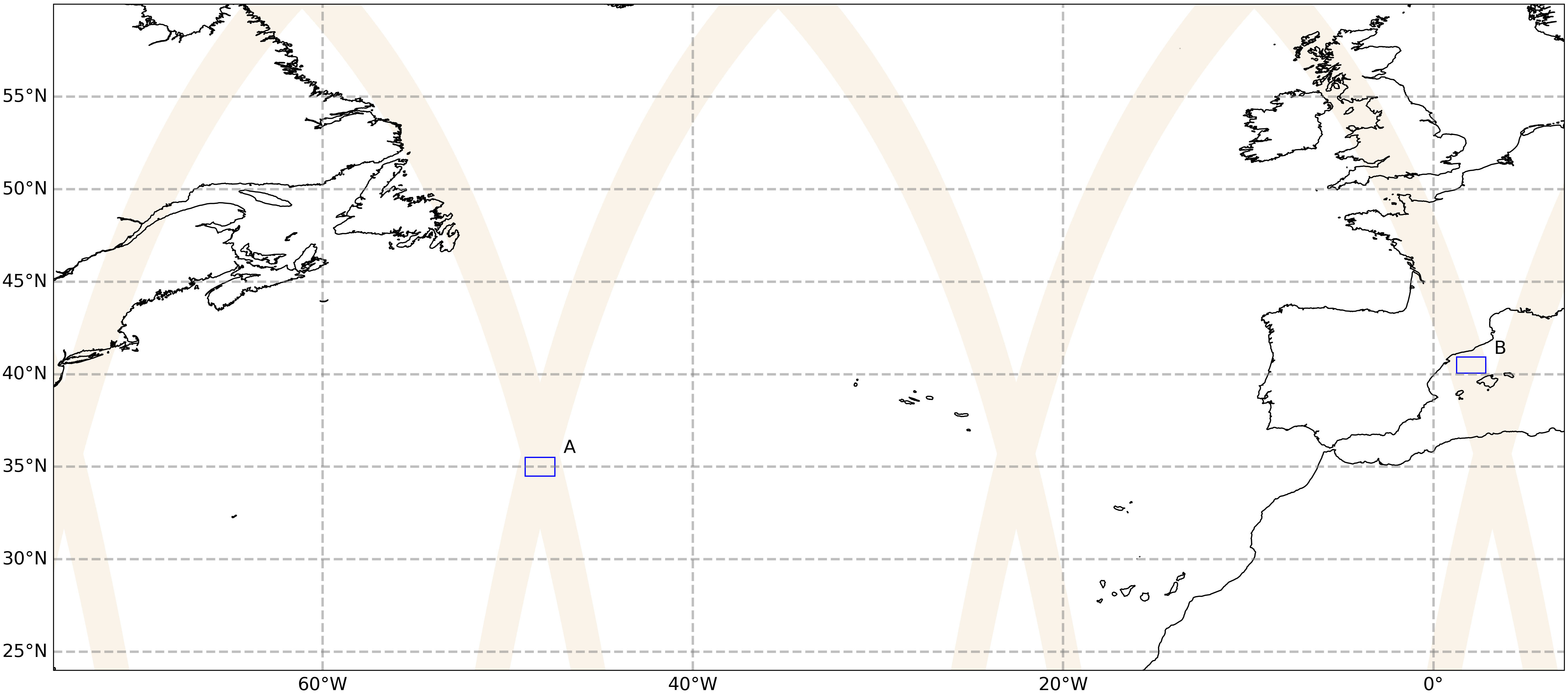
Figure 1 Training area (A) and testing area (B) presented with the SWOT passages in the fast-sampling phase. The coordinates of the SWOT passages comes from the simulated SWOT product from the MITgcm LLC4320 model (L2 LR SSH), available on the AVISO website: http://doi.org/10.24400/527896/a01-2021.006.

For simplicity, our approach assumes a synoptic scenario, where all observations occur simultaneously. Future work will address the non-synoptic nature of actual sampling and explore how the network accommodates this. Furthermore, in this study, we did not incorporate simulated noise or measurement errors into our data, opting to explore these aspects in subsequent research. Despite this, the practical effectiveness of our network is demonstrated through tests using actual observational data, details of which are provided in the following subsection.

2.2 Real observations

2.2.1 Remote-sensing observations

In our study, we have used Sea Surface Temperature (SST) and Ocean Color (CHL) imagery from the 18th of February, 2022, distributed by CMEMS. The CHL has 1 km spatial resolution, and it is a level-3 product obtained by multi-Sensor processing from OceanColor (Volpe et al., 2019). The SST also has a 1 km spatial resolution and it is based on level-2 product based on multi-channel sea surface temperature (SST) retrievals, which it has generated in real-time from the Infrared Atmospheric Sounding Interferometer (IASI) on the European Meteorological Operational-A (MetOp-A) satellite.

2.2.2 Glider observations

Gliders are autonomous underwater vehicles that allow sustained collection at high spatial resolution (1 km) and low costs compared to conventional oceanographic methods. Many studies confirmed the feasibility of using coastal and deep gliders to monitor the spatial and low-frequency variability of the coastal ocean (Alvarez et al., 2007; Heslop et al., 2012; Ruiz et al., 2019; Zarokanellos et al., 2022). In this work we used the observations from two gliders in the Balearic Sea as a part of the Calypso 2022 experiment. The two gliders carried out a suite of sensors that measure temperature, conductivity and pressure (CTD), dissolved oxygen (oxygen optode), Chlorophyll fluorescence and Turbidity (FNLTU). The two gliders were programmed to profile from the surface up to 700 m with a vertical speed of 0.18 ± 0.02 m/s and moved horizontally at approximately 20–24 km per/day. Data were processed following the methodology described in Troupin et al. (2015). In this study, we have used the temperature data at 15 m from the 10th of February until the 18th of February.

3 Methods

When sparse observations are available, the most common technique that has been adopted in oceanography and in different fields of science using a gridded product is Optimal Interpolation (OI) (Gandin, 1966). The technique relies on a solid mathematics basis and has been the state-of-the-art approach for many geophysical products until now. Since the proposed neural approach and specifically our prior builds over the OI framework we reviewed it in subsection 3.1. Then, we introduce CLOINet our neural approach and its submodules in subsection 3.2. Lastly, we present the metrics we used for bench-marking purposes.

3.1 Baseline: OINet

A common approach to explain the OI math start considering y as the vector containing all the observations we have of the true state x, which is unknown. We can relate them with the following observation model Equation 1:

$\begin{array}{ll}\mathbf{\text{y}}=\mathbf{\text{Hx}}+ϵ& (1)\end{array}$

where H is the observation (or masking) operator, and ϵ is the observation error. Under Gaussian hypotheses for ϵ and the prior on x, we can obtain the best possible estimation of true state x_s given the observations y through a linear operator K (the Kalman gain see Welch and Bishop (1995)):

$\begin{array}{ll}{\mathbf{\text{x}}}^s=\mathbf{\text{Ky}}& (2)\end{array}$

$\begin{array}{ll}\mathbf{\text{K}}=\mathbf{\text{B}}{\mathbf{\text{H}}}^T{(\mathbf{\text{H}}\mathbf{\text{B}}{\mathbf{\text{H}}}^T+\mathbf{\text{R}})}^{-1}& (3)\end{array}$

where R is the observation error covariance matrix and B is the error covariance specific of the analysis. In Equation 3, we are assuming an a-priori knowledge of both R and B, which could be theoretically obtained by repeating the same experiments many times. Practically, a parameterized covariance matrix is often used to substitute the complete climatology covariances Gaspari and Cohn (1999). The most common parametrization for this matrix is a Gaussian-shaped correlation, depending only on the points’ distances and pre-determined correlation lengths. So for two generic position vectors r_i and r_j, we have:

$\begin{array}{ll}{\mathbf{\text{B}}}_{i,j}=cov(r_i,r_j)=e^{-{\displaystyle {\sum }_{n=1}^3\frac{{(r_{i,n}-r_{j,n})}^2}{2c_n^2}}}& (4)\end{array}$

where the sum for dimension n considers the squared difference of the components of the position vectors r_i,n and r_j,n divided by the squared nth correlation length c_n. Regarding the observation error matrix, we assume from now on that it is diagonal Equation 5:

$\begin{array}{ll}{\mathbf{\text{R}}}_{i,j}={\mathbf{\text{I}}}_{i,j}ϵ& (5)\end{array}$

A different case where the observation errors are correlated is possible. However, R is often assumed diagonal to reduce computational costs (Miyoshi and Kondo, 2013). Finally, inserting B and R in Equation 3 and then in Equation 2 we can compute our estimated field x^s.

In our experiments, we established a baseline method with OINet, a simple neural network, that automatically discover the OI correlation lengths among different variables (SST, SSH, and salinity) and dimensions. OINet is then provided with the same input data as CLOINet, including surface fields (SST and/or SSH) and in-situ salinity observations. It operates in a two-step process: the first step involves transforming the multivariate surface fields into a unified field, making it compatible for being used with the salinity observations. The second step is to estimate the three correlation lengths specific to the current set of observations. While the first step involves 2 convolutional layers the second one is a simple feed-forward neural networks able to process a generic number of O observations (see the bottom part of Figure 2).

Figure 2

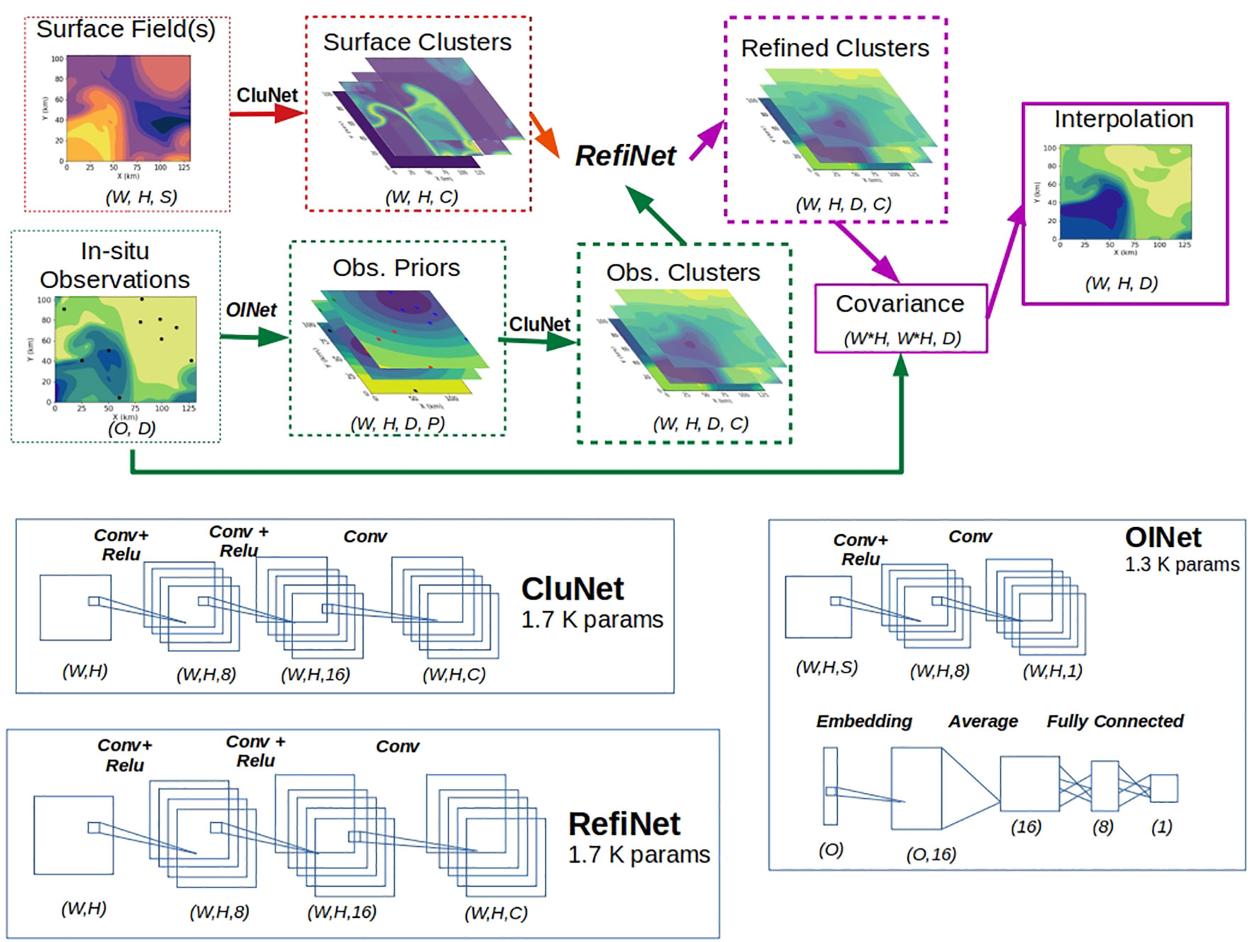
Figure 2 Flow chart of CLOINet information processing: Red and green elements (boxes and arrows) represent the processing paths for the SST input surface field and the in-situ salinity observations, respectively. Purple elements indicate the combined use of both inputs. The bold text along the arrows specifies the network module in operation. The line style and width of each box vary to represent different processing stages, ranging from thin and dashed for inputs to solid and thick for outputs. Inside each box, capital letters denote the corresponding tensor dimensions: W for field width, H for field height, S for the number of input surface fields, P for the number of OINet priors, C for the number of clusters (consistent across all modules in our tests), D for the number of depths, and O for the number of in-situ observations. Colorbars are omitted for clarity. The lower part of the image illustrates the CNN architecture of the three modules, along with the number of parameters used.

Beyond the parameter estimation this module is simply realizing an OI using the formula in Equation 4 to calculate the covariances. Notably this approach not only automates the tuning of parameters but also leverages GPU power for more efficient interpolation computations.

3.2 CLuster enhanced Optimal Interpolation Network

Ocean dynamics often display non-local and anisotropic patterns, which traditional Optimal Interpolation (OI) methods struggle to account for effectively. The main challenge with OI lies in its correlation function assumptions, which may not accurately reflect the actual physical conditions of the ocean. For instance, as seen in Equation 4 OI typically presumes that points in close proximity are strongly correlated, while distant points are not. However, oceanographic phenomena can exhibit the opposite behavior. For example, ocean fronts, characterized by narrow zones with strong horizontal density gradients, act as boundaries between water masses with distinct physical and bio-optical properties. Conversely, in dynamic ocean features like meanders and eddies, water masses can remain similar over vast distances.

Here, we aim to benefit from the wealth of information from remote sensing regarding the shape of the ocean features, whether they belong to the mesoscale or the submesoscale. The key idea is grouping a set of objects in such a way that each object is more similar to the objects belonging to its same group (called a cluster) than the rest. This procedure in statistics is called clustering. Applying this concept to reconstructing the ocean state, our approach is to reveal non-local correlations by clustering grid points that are part of the same oceanic features. This led us to develop CLOINet (Cluster-enhanced Optimal Interpolation Net), an end-to-end system designed to optimally interpolate sparse in-situ observations using available remote-sensing images. CLOINet is able to process any kind of surface fields (2D images) and in-situ observations (2D masks and observation values). Its main submodule is CLuNet, which transforms 2D fields into fuzzy clusters. While satellite images could directly been passed to this module in-situ observation profiles are initially processed by OINet, which serves as a prior, converting them into images. Finally a further submodule, RefiNet, module merges the fuzzy clusters from both surface fields and observation priors into a final cluster set. Within this latent cluster space an alternative distance could replace the euclidean distance allowing a better estimation of B and consequently obtains the reconstructed field x^s.

Our network structure allows a joint training of all modules, minimizing their specific loss function terms summed up in a global loss function. Convolutional Neural Networks (CNN) layers. Here following, we describe the details of the network submodules and how we obtained the interpolation in an end-to-end scheme also summarized in Figure 2).

3.2.1 Clusters space transformation: CluNet

The first module of our scheme, called CluNet is in charge of transform any images into a set of clusters. Piratically speaking it segments the input 2D images (like multivariate remote-sensing fields or the observations priors) into C clusters of similar points. In this context, we consider two points similar according to their positions (as in Equation 4) but also their values in the input 2D fields. In particular, we worked within the so-called “fuzzy logic”, where the membership function m_jk, which expresses how much the j point belongs to the k cluster, could assume every value between 0 and 1. Considering this continuous range means that each grid point could be part of more than one cluster as long as the following normalization holds:

$\begin{array}{ll}{\displaystyle \sum _{k=1}^C{m}_{jk}=1} \forall j& (6)\end{array}$

For its non-binary logic, this clustering technique is called “Fuzzy Clustering” or soft k-means. being this last the simpler binary case in which m_jk could be just 1 or 0. CluNet takes the remote-sensing images as input and gives the tensor composed by all the m_jk through various CNN and finally a softmax layer to guarantee Equation 6. The associated training loss, referred to as a Robust fuzzy C-means (Chen et al., 2021) loss, is composed of two terms:

$\begin{array}{ll}{ℒ}_{RFCM}(\mathbf{\text{y}};\theta )={\displaystyle \sum _{j\in \Omega }{\displaystyle \sum _{ k=1}^C{m}_{jk}^q(\mathbf{\text{y}};\theta )}}{\Vert y_j-v_k\Vert }^2+\beta {\displaystyle \sum _{j\in \Omega }{\displaystyle \sum _{ k=1}^C{m}_{jk}^q(\mathbf{\text{y}};\theta )}}{\displaystyle \sum _{l\in N_{j}m\in M_k}{\displaystyle \sum _{lm}{m}_{lm}^q}}(\mathbf{\text{y}};\theta )& (7)\end{array}$

y is the vector containing the surface field that we want to cluster with y_j its value at point j in our domain Ω. q is a parameter that satisfies q ≥ 1 and controls the amount of fuzzy overlap between clusters. Minimizing the first term achieves that points with high membership function for the k cluster should be similar to its center v_k defined as follows Equation 8:

$\begin{array}{ll}{v}_k=\frac{{\sum }_{j\in \text{Ω}}{m}_{jk}^q(\mathbf{\text{y}};\theta )y_j}{{\sum }_{j\in \text{Ω}}{m}_{jk}^q(\mathbf{\text{y}};\theta )}& (8)\end{array}$

The second term guarantees the membership function’s spatial smoothness, forcing the j point to have a similar value to its neighborhood N_j. The parameter β controls the intensity of this constraint.

In summary, to obtain the clustering, we minimize Equation 7 with respect to the parameters of the CNN layers included in CluNet, which stand in the θ vector. Since in this loss term, we do not directly provide any ground truth (i.e., the best way of clustering the inputs), this part of the network could be considered self-supervised since it learns indirectly from the rest of the loss term. As it show in Figure 2 we used this module twice, firstly for clustering surface input fields and secondly for clustering the 2D fields coming from the observations priors described hereafter. Consequently in the global loss there are two terms like Equation 7.

3.2.2 Observations priors

We have outlined the process by which CluNet segments any set of 2D fields into distinct clusters. To handle in-situ observations, which are essentially vectors of observations at different depths, we utilize OINet to convert them into a series of images that can then be clustered. As previously mentioned, OINet has the capability to autonomously determine the appropriate correlation lengths for a given set of observations and then perform a canonical Optimal Interpolation (OI). In our approach, we generate four different versions of these interpolations, each initiated with correlation lengths that are submultiples of the domain sizes. These parameters, among others, are then fine-tuned during the learning phase. This process results in four fields that CluNet subsequently clusters into areas exhibiting similar values, despite being derived using different correlation lengths. The clusters formed from these observations provide insights into the certainty we have about specific regions and the extent to which a particular depth is influenced by surface conditions. Essentially, this method allows us to address potential anisotropy in the uncertainties without having to rely on fixed length scales.

3.2.3 Data fusion in the clusters space: RefiNet

We now have a set of clusters derived from the surface fields, and an additional set for each depth of the in-situ observations. For each depth, the corresponding sets of surface and observation clusters are processed through RefiNet. The resulting clusters, along with their membership vectors, are used to compute the covariance matrix as follows Equation 9:

$\begin{array}{ll}{\mathbf{\text{B}}}_{i,j}=cov(r_i,r_j)=1-\sum _{k=1}^C{({m^{\prime }}_{ik}-{m^{\prime }}_{jk})}^2& (9)\end{array}$

In this equation, we sum the differences in the membership functions of points ii and jj across all clusters. This process, while bearing similarities to Equation 4 deviates by using subtraction instead of an exponential function since m_ik and m_jk are already bounded within the 0-1 range. This summation represents a non-local distance in the cluster space, replacing the classical Euclidean distance. Consequently, two points within the same cluster (i.e., with similar membership vectors) will be correlated, regardless of their spatial distance.

Using parametrization (9), we then compute the associated optimal interpolation as Equation 3 and then Equation 2. This forms an end-to-end architecture that uses remote sensing images and in-situ data to output regularly-gridded vertical profiles (see Figure 2 for the data flow).

The training loss combines three components: two clustering-based losses Equation 7 (one for the surface fields and one for the observations priors) and a supervised reconstruction term. So globally we minimize Equation 10:

$\begin{array}{ll}ℒ=\alpha {ℒ}_{sr{f}_{R}FCM}+\beta {ℒ}_{ob{s}_{ R}FCM}+\text{γ}{ℒ}_{MSE}& (10)\end{array}$

where α, β and γ are the weights of the three loss terms, and L_MSEis given by Equation 11:

$\begin{array}{ll}{ℒ}_{MSE}={({\mathbf{\text{x}}}^s-\mathbf{\text{x}})}^2& (11)\end{array}$

This last term is just the mean squared error with respect to the ground truth x. Within the considered supervised training strategy, self-supervised losses Equation 7 act as regularization terms to improve generalization performance and explainability. We maintain equal weights of α, β, and γ at 1, as no significant differences were observed with other values. Our network also shows relative insensitivity to other hyperparameters, such as the number of clusters. However, our cross-validation tests indicated that setting this number to 20 yielded the best results.

3.3 Performance metrics

To understand how the clusters sets were changing according to the input data we computed the associated entropy fields. In fact, given that the membership vector is normalized and thus it can be seen as a distribution, its entropy definition is Equation 12:

$\begin{array}{ll}Si=-{\displaystyle \sum _{k=1}^C{m}_{ik}^{\prime } \text{log}{m}_{ik}^{\prime }}& (12)\end{array}$

To assess the performance of the proposed approach, we first define the error between the ground truth and the estimated field value Equation 13:

$\begin{array}{ll}{\mathbf{\text{x}}}_{err}=\mathbf{\text{x}}-{\mathbf{\text{x}}}_s& (13)\end{array}$

then we easily obtain our first performance metric: the Root Mean Squared Error (RMSE) Equation 14:

$\begin{array}{ll}RMSE=\sqrt{x_{err}^2}& (14)\end{array}$

We will present this metric in percentage of the standard deviation of the ground truth fields. Now considering the standard deviation of the error over the whole N snapshot Equation 15:

$\begin{array}{ll}{\sigma }_{err}=\frac{{\sum }_{t=1}^N{\left(x_{err}(t)-\overline{x_{err}(t)}\right)}^2}{N}& (15)\end{array}$

we can compute the explained variance score dividing by the standard deviation of the ground truth Equation 16.

$\begin{array}{ll}{\sigma }_S(x,y)=1-\frac{{\sigma }_{err}}{{\sigma }_{true}}& (16)\end{array}$

To highlight the effective resolution of the different reconstruction methods we use the noise-to-signal ratio NSR (Ballarotta et al., 2019) Equation 17:

$\begin{array}{ll}NSR(\text{λ})=\frac{PSD(x_{err},\text{λ})}{PSD(x,\text{λ})}& (17)\end{array}$

the effective resolution is in fact given by the wavelength λ_s where the NSR λ_s is 0.5.

4 Results and discussion

This section first reports numerical experiments using NATL60 OSSEs to evaluate the proposed approach quantitatively. The concluding subsection presents an application to real observations.

4.1 Clusters entropy

The initial part of our analysis focuses on understanding how CLOINet, via CluNet and subsequently RefiNet, organizes clusters based on different data inputs: SST, SSH, and various sets of randomly located in-situ salinity observations. To illustrate this, we plotted some example entropy fields in Figure 3 along with statistics on how entropy changes with an increasing number of observations N. In the four panels on the left side of Figure 3 we display two clusters’ entropy fields (panels a and e) and their corresponding input fields for SSH (panel b) and SST (panel f) from a selected snapshot. In the four panels on the right side, we present the entropy associated with the in-situ observations’ clusters at two different depths z = 5 (panel c) and z = 150m (panel g) together with the correspondent refined clusters entropy (panel d and h) along with the refined clusters’ entropy (panels d and h).

Figure 3

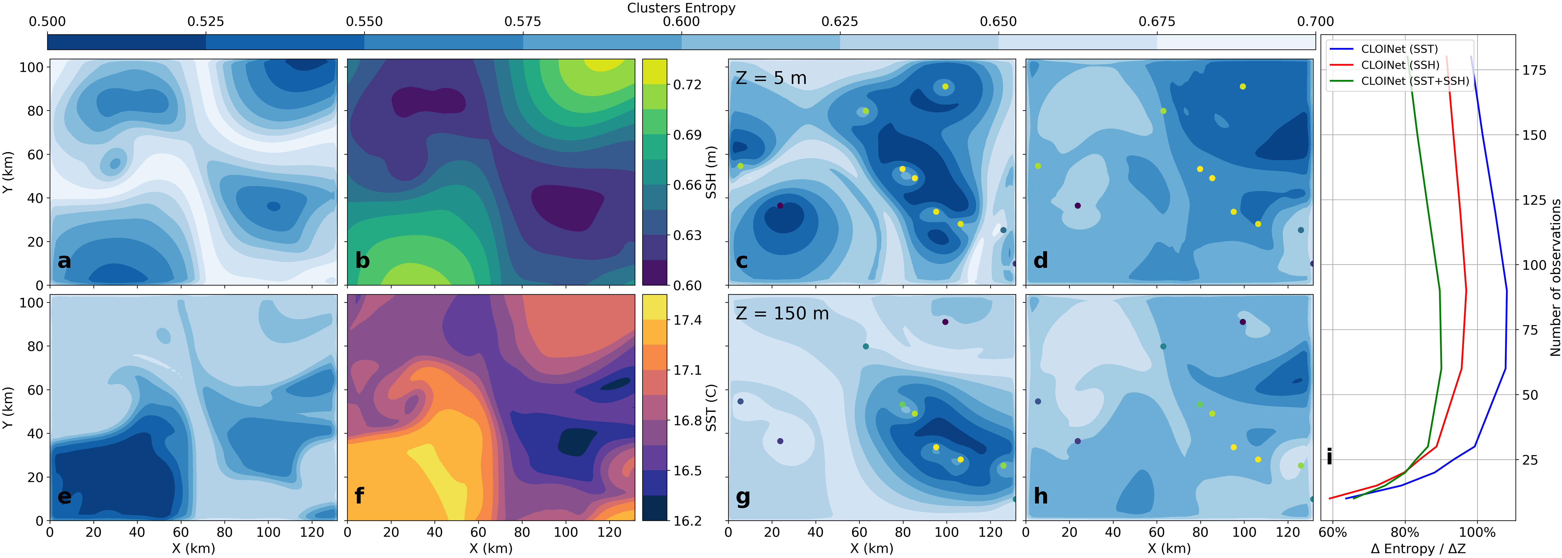
Figure 3 The entropy of the cluster sets, resulting from the input SSH and SST, is depicted in panels a and e, respectively, while the corresponding fields themselves are shown in panels b and f. Panels c and d (and g and h) display the entropy of the observation and refined cluster sets at a depth of Z = 5 m and Z = 150 m, respectively. The dots in these panels represent salinity observations at these depths, with their colors indicating the magnitude of salinity (scale not shown). Panel i illustrates the variation in the entropy of the refined cluster sets along the vertical axis, corresponding to different numbers of observations. The varying colors in this panel represent different networks.

This particular snapshot was chosen for its submesoscale features. The differences between SSH and SST-based entropy are noticeable; the SSH clusters highlight more prominent features, while SST forms smaller clusters that extend to deeper depths. The correspondence between the surface fields and their cluster entropy is relatively straightforward, but differences in other sets are more subtle. For observation clusters’ entropy, we observe lower entropy (blue regions) near points with similar observations. Areas of higher entropy occur between two observation points with differing values. This behavior varies at different depths, explaining the differences between panels c and d. The refined clusters, influenced by both observations and surface fields, exhibit subtler changes, but we can still see an increase in entropy with depth, particularly noticeable in the northeast region of panels d and h.

Beyond this specific snapshot, panel i shows the percentage change in entropy between the two depths, averaged across the entire test dataset as a function of the number of observations. When only SST data is available, the changes in clusters are more pronounced, as SST information is less directly related to the ocean’s interior compared to SSH or combined SST and SSH data. As expected, all deltas increase with the number of observations, eventually reaching a saturation point where they decrease. This occurs because the clusters’ information becomes less critical, and the field can be reconstructed relying primarily on in-situ observations.

4.2 RMSE and correlation

WWe present the outcomes of the random sampling OSSE in Figure 4. The first two rows illustrate a ground truth salinity example at two different depths, alongside the reconstructions by the baseline OINet and CLOINet with various surface input fields. Again, we chose the same snapshot from Figure 3 for its distinct submesoscale features.

Figure 4

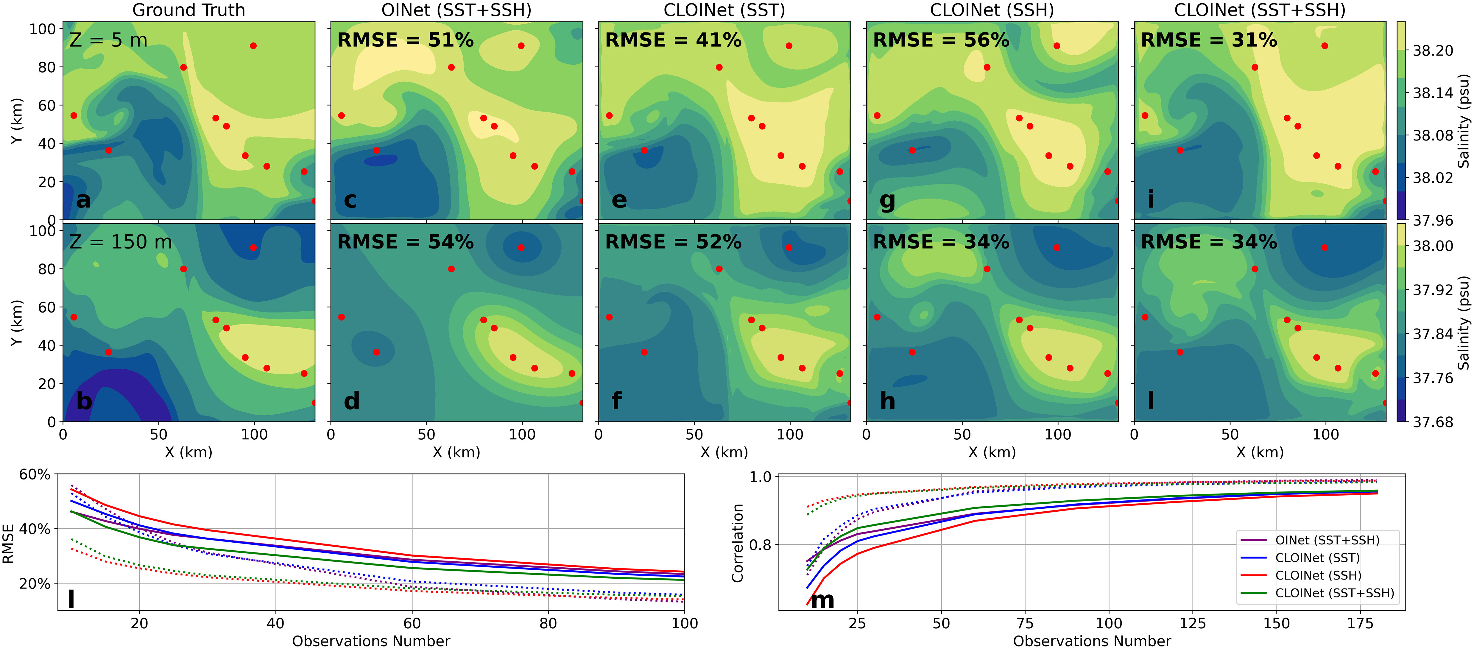
Figure 4 Example of salinity field interpolation at Z = 5m (first row, panels A, C, E, G, I) and Z = 150m (second row, panels B, D, F, H, I) with ten random observations. The first column shows the ground truth, and the subsequent columns represent various interpolation methods. The two bottom plots display the RMSE (panel L) and correlation coefficient (panel M) as functions of the number of observations in a random sampling scenario, averaged across the entire test dataset. In these plots, the solid line corresponds to Z = 5m, while the dashed line represents Z = 150m.

OINet can effectively use surface information for reconstructing the surface layer, but it struggles to propagate this information to deeper layers. We also experimented forcing a bigger correlation length in the z axis but we ended up with a reversed scenario: a well-reconstructed bottom layer but a poorly reconstructed (not shown). This limitation arises because the simple network cannot determine which surface fields to prioritize based on the in-situ observations.

In the case of CLOINet, we observe different results based on the input fields provided. SST leads to better surface interpolations, while SSH is more effective for deeper fields. This outcome aligns with our expectations, as SSH data is depth-integrated and thus more informative than SST for understanding the shape of water masses at depth. Notably, when both SST and SSH are used as inputs, the network effectively leverages their shape information to enhance both surface and interior reconstructions, leading to a reduction in RMSE by about 40% at both depths.

The results across the entire testing set show similar patterns. On panel l (m) we show how for all methods, the RMSE (correlation) decreases (increases) in proportion to the number of observations. In these plots, solid lines represent surface salinity fields, while dashed lines indicate interior fields at z = 150m. Interestingly, on average, OINet’s performance is comparable to CLOINet’s for surface reconstructions but falls short for interior reconstructions. This fact is mostly related with presence or not of submesoscale features as the next subsection analysis will show. The variation in CLOINet’s surface inputs shows minimal impact on surface results, with only slight improvements observed in the SST+SSH case. However, the introduction of the SSH field significantly enhances the interior field reconstructions. Once again, this confirms that SSH provides more comprehensive information about the entire water column compared to SST.

4.3 Resolved scales

In Figure 5, we present the results of the OSSE conducted with regular grid sampling, varying the spacing between observations to understand how different methods resolve various spatial scales. Specifically, we examined the impact of sampling resolution on the explained variance and the Power Spectral Density (PSD)-based score. The explained variance for the different reconstruction methods at a sampling resolution of 20 km is shown in panels a, c, e, and g (and panels b, d, f, and h for the interior field). When provided with the same inputs as OINet (SST and SSH), CLOINet slightly surpasses it on the surface and by about 20% in the interior. Again, we observe superior performance from CLOINet-SSH in the interior, while the inferior performance of the network relying solely on SST suggests that, on average, this field does not significantly account for salinity variability.

Figure 5

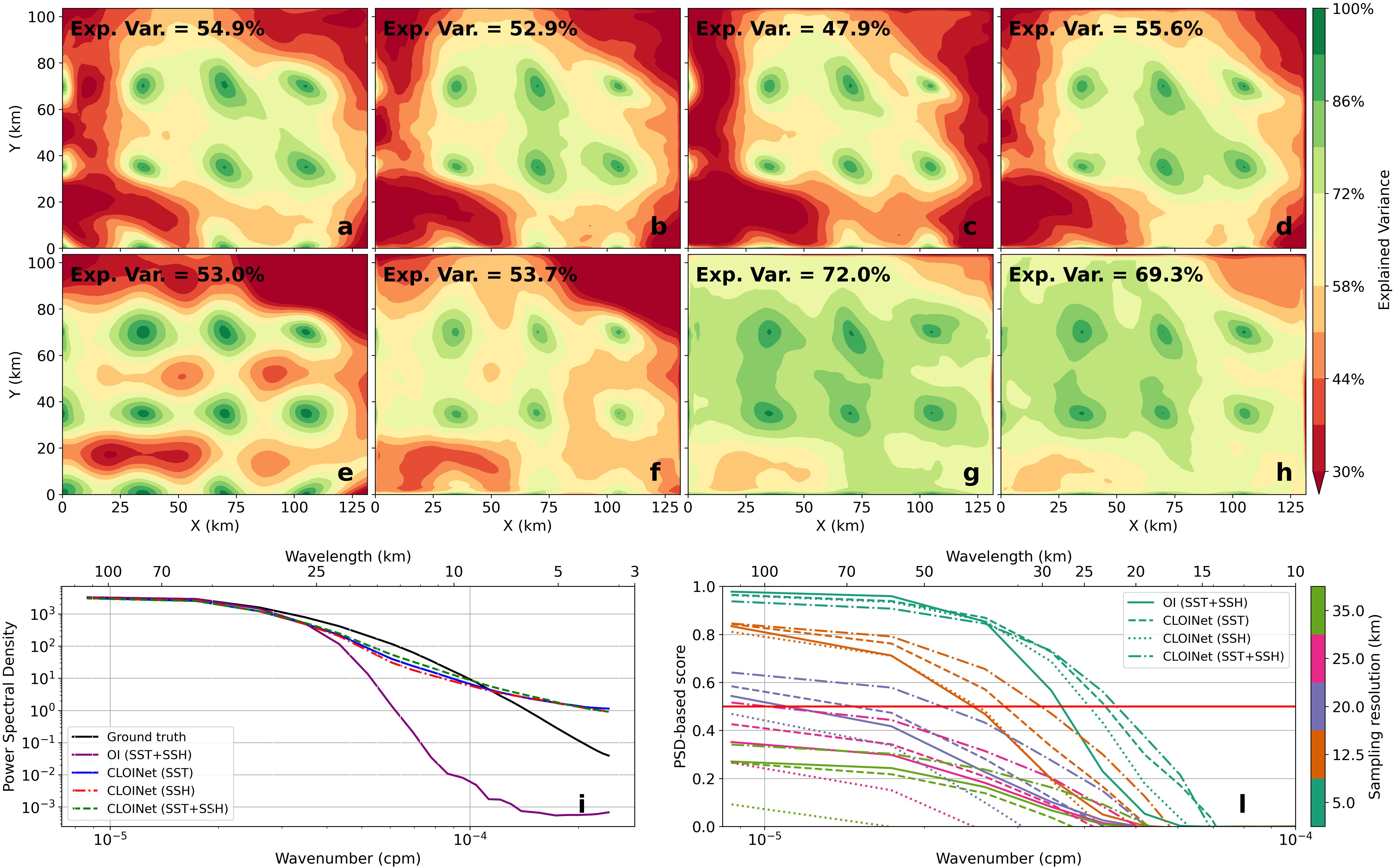
Figure 5 This figure shows the explained variance for various interpolation methods averaged across the entire test dataset, in a scenario with regular sampling at 45 km intervals. Panels (A-D) display the results at Z = 5m for OI, CLOINet-SST, CLOINet-SSH, and CLOINet-SST+SSH, respectively, panels (E-H) are instead relative to Z = 150m. Black dots mark the locations of in-situ observations while the spatial average value for each method is indicated on the corresponding subplot. Panel (I) compares the Power Spectral Density (PSD) of the different reconstruction methods with the ground truth, with each color representing a different method. Panel (L) shows the corresponding score, where the colors denote different sampling resolutions. In both panels (I, L), solid lines represent surface fields, while dashed lines correspond to fields at a depth of z = 150m. The red line across panel (L) marks the 0.5 threshold value, indicating the effective resolution of the interpolation methods.

The PSD-based score, shown in panel l, indicates the effective resolution of the reconstruction (the point at which the score falls below 0.5) demonstrating how CLOINet generally resolves smaller scales than OINet across various sampling resolutions. For higher resolutions, such as 5 and 12 km, CLOINet resolves scales approximately 1.5 times larger than OINet. The training set’s averaged spectra, depicted in panel i, reveal that OINet is typically limited to reconstructing larger scales. Indirectly, this suggests that the variability explained in the test region is predominantly due to larger scales, which even OINet can adequately account for.

4.4 Real ocean data preliminary tests

In line with many deep learning studies, our research focuses on applying neural networks, initially trained on synthetic data, to real-world observations. We evaluated CLOINet’s effectiveness in improving Sea Surface Temperature (SST) estimates using glider surface temperature observations, enhanced with shape information from a Chlorophyll (CHL) snapshot (refer to Figure 6). Both OINet and CLOINet were able to reconstruct the general SST pattern observed in reality. CLOINet demonstrated a slightly superior performance, as evidenced by higher correlation values. This improvement aligns with our qualitative observations, suggesting that CLOINet more accurately preserves submesoscale features. Notably, this achievement was realized without the networks being specifically trained on CHL data. In these preliminary tests, the CHL data was provided as if it were the SST and SSH fields, demonstrating the networks’ versatility in utilizing shape information from various types of variables. Achieving similar levels of accuracy with traditional Optimal Interpolation (OI) methods would be more complex, likely necessitating intricate, predefined multi-variate correlation functions and extensive parameter tuning.

Figure 6

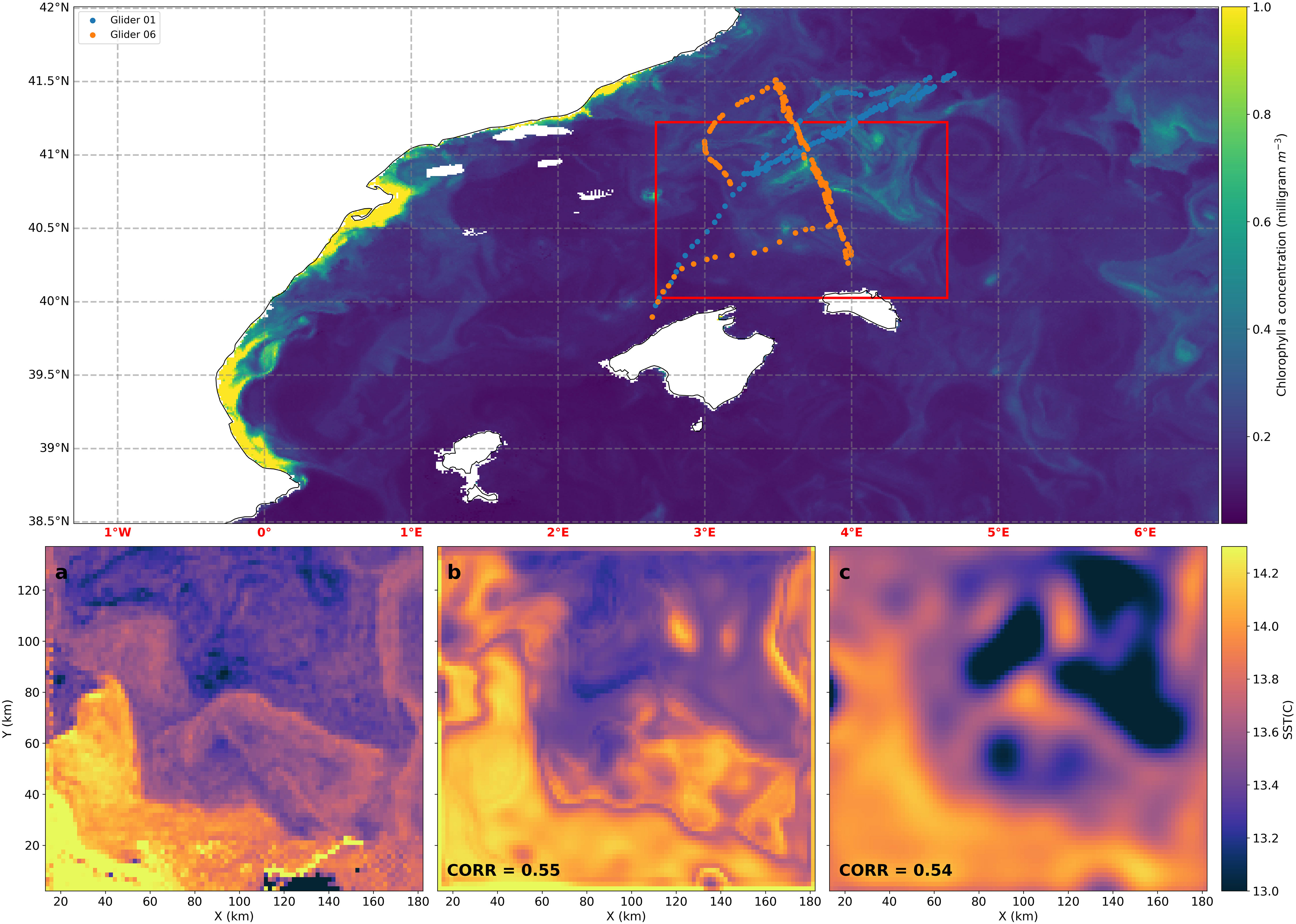
Figure 6 The top panel displays the Chlorophyll-a (CHL-a) concentration in the Western Mediterranean Sea on February 18, 2022. The dots represent temperature observations from two gliders over the preceding 48 hours, while the red box outlines the area where interpolation was performed. The bottom panels, labeled a, b, and c, show the actual Sea Surface Temperature (SST) this same day and the reconstructed SST using CLOINet and OINet, respectively. The correlation values for each reconstruction method are indicated in the corresponding plots.

5 Conclusion

In this, we presented CLOINet, a comprehensive end-to-end neural network designed to combine sparse in-situ observations into a full 3D field leveraging shape information from kind of ocean remote sensing images. We conducted end-to-end training of CLOINet within a supervised framework, using Observing System Simulation Experiments (OSSEs) based on the NEMO-derived NATL60 simulation. Our study focuses on comparing the reconstruction of 3D salinity capabilities of CLOINet with those of a data-driven version of classical Optimal Interpolation, which we have named OINet. This comparison also extends to applications involving real observational data.

Our research covered various scenarios, including both randomly and regularly spaced in-situ salinity observations, paired with different remote sensing inputs such as Sea Surface Temperature (SST), Sea Surface Height (SSH), or a combination of both. Upon creating a 3D salinity field, we thoroughly analyzed how our performance metrics responded to variations in the number and density of in-situ observations.

In dense regular sampling we showed how CLOINet was able to resolve scales 1.5 smaller scales compared to OINet while in random sampling contexts, CLOINet showed enhanced performance in terms of both RMSE and correlation, especially notable when limited observations were available. This improvement was significant in scenarios involving in-depth fields and areas rich in submesoscale features, where RMSE improvements reached as high as 40%.

Despite not incorporating simulated errors to mimic actual sampling instruments, the promising results with real data highlight the potential of our approach in operational contexts. In fact, CLOINet adeptly handled noisy CHL fields and gliders in-situ temperature and successfully reconstructed the general pattern of an unseen SST field, without specific training for this task. These outcomes also demonstrate that, apart from reconstructing salinity, the process of transforming input data into a latent space composed of clusters enables comprehensive multi-variate analysis.

Our training approach, which combined two self-supervised losses with a supervised reconstruction loss, enabled the network to generalize effectively. This was evident as it performed accurately in the Western Mediterranean test area, distinctly different from the North Atlantic training region. This suggests that our method is not limited by specific regional climatology and could potentially be scaled for global application.

Overall, the modular design of CLOINet not only enhances our understanding of its internal processes but also positions it for future enhancements. One promising direction for subsequent research is extending the model to incorporate space-time dynamics. Another intriguing possibility is employing this neural network approach for guiding an adaptive sampling multi-platform ocean campaign. Given the significant role of SSH data in assessing the reconstruction of the deeper water layers, the upcoming high-resolution SSH observations from SWOT present an exciting opportunity for further refining and applying CLOINet.

Additional requirements

For additional requirements for specific article types and further information please refer to AuthorGuidelines.

Data availability statement

The raw data supporting the conclusions of this article will be made available by the authors, without undue reservation.

Author contributions

EC, AP, SR, and RF contributed to conception and design of the study. EC developed the software CLOINet, performed the statistical analysis and wrote the first draft of the manuscript. NZ helped for writing the glider section. All authors contributed to the article and approved the submitted version.

Funding

The author(s) declare financial support was received for the research, authorship, and/or publication of this article. EC acknowledges support from the Spanish Ministerio de Ciencia e Innovacion (grant BES-2017-080763). This article is also a contribution to the PRE-SWOT and FAST-SWOT projects funded by the Spanish Research Agency and the European Regional Development Fund (AEI/FEDER, UE) under grant agreements (CTM2016-78607-P) and (PID2021-122417NB-I00) respectively. Furthermore AP and SR were funded by the CALYPSO project Office of Naval Research grant N0014-21-1-2702.

Acknowledgments

EC acknowledges the MEOM Research Group group for kindly providing the eNATL60 model outputs and all the members of the CALYPSO project for their comments and suggestions. EC acknowledges Prof. Carlos Granero Belinchon for engaging in valuable discussions that significantly enhanced the quality of the manuscript.

Conflict of interest

The authors declare that the research was conducted in the absence of any commercial or financial relationships that could be construed as a potential conflict of interest.

Publisher’s note

All claims expressed in this article are solely those of the authors and do not necessarily represent those of their affiliated organizations, or those of the publisher, the editors and the reviewers. Any product that may be evaluated in this article, or claim that may be made by its manufacturer, is not guaranteed or endorsed by the publisher.

References

Ajayi A., Le Sommer J., Chassignet E., Molines J. M., Xu X., Albert A., et al. (2020). Spatial and temporal variability of the North Atlantic eddy field from two kilometric-resolution ocean models. J. Geophys. Res.: Oceans. 125, e2019JC015827. doi: 10.1029/2019JC015827

CrossRef Full Text | Google Scholar

Alvarez A., Garau B., Caiti A. (2007). “Combining networks of drifting profiling floats and gliders for adaptive sampling of the Ocean,” in Proceedings - IEEE International Conference on Robotics and Automation, 157–162. doi: 10.1109/ROBOT.2007.363780

CrossRef Full Text | Google Scholar

Amores A., Jordà G., Arsouze T., Le Sommer J. (2018). Up to what extent can we characterize ocean eddies using present-day gridded altimetric products? J. Geophys. Res.: Oceans. 123, 7220–7236. doi: 10.1029/2018JC014140

CrossRef Full Text | Google Scholar

Arcucci R., Zhu J., Hu S., Guo Y. K. (2021). Deep data assimilation: integrating deep learning with data assimilation. Appl. Sci. 11, 1114. doi: 10.3390/APP11031114

CrossRef Full Text | Google Scholar

Arnold C. P., Dey C. H. (1986). Observing-systems simulation experiments: Past, present, and future. Bull. Am. Meteorol. Soc. 67, 687–695. doi: 10.1175/1520-0477(1986)067<0687:OSSEPP>2.0.CO;2

CrossRef Full Text | Google Scholar

Ballarotta M., Ubelmann C., Pujol M. I., Taburet G., Fournier F., Legeais J. F., et al. (2019). On the resolutions of ocean altimetry maps. Ocean. Sci. 15, 1091–1109. doi: 10.5194/OS-15-1091-2019

CrossRef Full Text | Google Scholar

Barth A., Alvera-Azcárate A., Licer M., Beckers J. M. (2020). DINCAE 1.0: A convolutional neural network with error estimates to reconstruct sea surface temperature satellite observations. Geosci. Model. Dev. 13, 1609–1622. doi: 10.5194/GMD-13-1609-2020

CrossRef Full Text | Google Scholar

Carrassi A., Bocquet M., Bertino L., Evensen G. (2018). Data assimilation in the geosciences: An overview of methods, issues, and perspectives. Wiley. Interdiscip. Rev.: Climate Change 9, e535. doi: 10.1002/WCC.535

CrossRef Full Text | Google Scholar

Charantonis A. A., Testor P., Mortier L., D’Ortenzio F., Thiria S. (2015). Completion of a sparse GLIDER database using multi-iterative self-organizing maps (ITCOMP SOM). Proc. Comput. Sci. 51, 2198–2206. doi: 10.1016/J.PROCS.2015.05.496

CrossRef Full Text | Google Scholar

Chen J., Li Y., Luna L. P., Chung H. W., Rowe S. P., Du Y., et al. (2021). Learning fuzzy clustering for SPECT/CT segmentation via convolutional neural networks. Med. Phys. 48, 3860–3877. doi: 10.1002/MP.14903

PubMed Abstract | CrossRef Full Text | Google Scholar

Contractor S., Roughan M. (2021). Efficacy of feedforward and LSTM neural networks at predicting and gap filling coastal ocean timeseries: oxygen, nutrients, and temperature. Front. Mar. Sci. 8. doi: 10.3389/FMARS.2021.637759/BIBTEX

CrossRef Full Text | Google Scholar

Cutolo E., Pascual A., Ruiz S., Johnston T. S., Freilich M., Mahadevan A., et al. (2022). Diagnosing frontal dynamics from observations using a variational approach. J. Geophys. Res.: Oceans., e2021JC018336. doi: 10.1029/2021JC018336

CrossRef Full Text | Google Scholar

Durack P. J., Gleckler P. J., Landerer F. W., Taylor K. E. (2014). Quantifying underestimates of long-term upper-ocean warming. Nat. Climate Change 4, 999–1005. doi: 10.1038/NCLIMATE2389

CrossRef Full Text | Google Scholar

Fablet R., Chapron B., Drumetz L., Mémin E., Pannekoucke O., Rousseau F. (2021). Learning variational data assimilation models and solvers. J. Adv. Modeling. Earth Syst. 13, e2021MS002572. doi: 10.1029/2021MS002572

CrossRef Full Text | Google Scholar

Fablet R., Drumetz L., Rousseau F. (2020). Joint learning of variational representations and solvers for inverse problems with partially-observed data. doi: 10.48550/arxiv.2006.03653

CrossRef Full Text | Google Scholar

Fresnay S., Ponte A. L., Le Gentil S., Le Sommer J. (2018). Reconstruction of the 3-D dynamics from surface variables in a high-resolution simulation of North Atlantic. J. Geophys. Res.: Oceans. 123, 1612–1630. doi: 10.1002/2017JC013400

CrossRef Full Text | Google Scholar

Gandin L. S. (1966). Objective analysis of meteorological fields. Translated from the Russian. Jerusalem (Israel Program for Scientific Translations), 1965. Pp. vi, 242: 53 Figures; 28 Tables. £4 1s. 0d. Q. J. R. Meteorol. Soc. 92, 447–447. doi: 10.1002/QJ.49709239320

CrossRef Full Text | Google Scholar

Gaspari G., Cohn S. E. (1999). Construction of correlation functions in two and three dimensions. Q. J. R. Meteorol. Soc. 125, 723–757. doi: 10.1002/qj.49712555417

CrossRef Full Text | Google Scholar

Gomis D., Ruiz S., Pedder M. A. (2001). Diagnostic analysis of the 3D ageostrophic circulation from a multivariate spatial interpolation of CTD and ADCP data. Deep. Sea. Res. Part I.: Oceanogr. Res. Papers. 48, 269–295. doi: 10.1016/S0967-0637(00)00060-1

CrossRef Full Text | Google Scholar

Gueye M. B., Niang A., Arnault S., Thiria S., Crépon M. (2014). Neural approach to inverting complex system: Application to ocean salinity profile estimation from surface parameters. Comput. Geosci. 72, 201–209. doi: 10.1016/J.CAGEO.2014.07.012

CrossRef Full Text | Google Scholar

Gurvan M., Bourdallé-Badie R., Chanut J., Clementi E., Coward A., Ethé C., et al. (2022). NEMO ocean engine. Tech. Rep. doi: 10.5281/ZENODO.6334656

CrossRef Full Text | Google Scholar

Hernandez-Lasheras J., Mourre B. (2018). Dense ctd survey versus glider fleet sampling: comparing data assimilation performance in a regional ocean model west of sardinia. Ocean. Sci. 14, 1069–1084. doi: 10.5194/os-14-1069-2018

CrossRef Full Text | Google Scholar

Heslop E. E., Ruiz S., Allen J., López-Jurado J. L., Renault L., Tintoré J. (2012). Autonomous underwater gliders monitoring variability at “choke points” in our ocean system: A case study in the Western Mediterranean Sea. Geophys. Res. Lett. 39. doi: 10.1029/2012GL053717

PubMed Abstract | CrossRef Full Text | Google Scholar

Jiang F., Ma J., Wang B., Shen F., Yuan L. (2021). Ocean observation data prediction for argo data quality control using deep bidirectional LSTM network. Secur. Commun. Networks 2021. doi: 10.1155/2021/5665386

CrossRef Full Text | Google Scholar

Manucharyan G. E., Siegelman L., Klein P. (2021). A deep learning approach to spatiotemporal sea surface height interpolation and estimation of deep currents in geostrophic ocean turbulence. J. Adv. Modeling. Earth Syst. 13, e2019MS001965. doi: 10.1029/2019MS001965

CrossRef Full Text | Google Scholar

Metref S., Cosme E., Le Guillou F., Le Sommer J., Brankart J. M., Verron J. (2020). Wide-swath altimetric satellite data assimilation with correlated-error reduction. Front. Mar. Sci. 6. doi: 10.3389/FMARS.2019.00822/BIBTEX

CrossRef Full Text | Google Scholar

Metref S., Cosme E., Le Sommer J., Poel N., Brankart J. M., Verron J., et al. (2019). Reduction of spatially structured errors in wide-swath altimetric satellite data using data assimilation. Remote Sens. 11, 1336. doi: 10.3390/RS11111336

CrossRef Full Text | Google Scholar

Miyoshi T., Kondo K. (2013). A multi-scale localization approach to an ensemble kalman filter. SOLA 9, 170–173. doi: 10.2151/SOLA.2013-038

CrossRef Full Text | Google Scholar

Morrow R., Fu L. L., Ardhuin F., Benkiran M., Chapron B., Cosme E., et al. (2019). Global observations of fine-scale ocean surface topography with the Surface Water and Ocean Topography (SWOT) Mission. Front. Mar. Sci. 6. doi: 10.3389/FMARS.2019.00232/BIBTEX

CrossRef Full Text | Google Scholar

Mourre B., De Mey P., Lyard F., Le Provost C. (2004). Assimilation of sea level data over continental shelves: an ensemble method for the exploration of model errors due to uncertainties in bathymetry. Dynamics. Atmospheres. Oceans. 38, 93–121. doi: 10.1016/J.DYNATMOCE.2004.09.001

CrossRef Full Text | Google Scholar

Pascual A., Macías D., Tintoré J., Turiel A., Ballabrera-Poy J., Castro C. G., et al. (2021). White Paper 13: Ocean science challenges for 2030 (Consejo Superior de Investigaciones Científicas (España).

Google Scholar

Pascual A., Ruiz S., Olita A., Troupin C., Claret M., Casas B., et al. (2017). A multiplatform experiment to unravel meso- and submesoscale processes in an intense front (AlborEx). Front. Mar. Sci. 4. doi: 10.3389/FMARS.2017.00039/BIBTEX

CrossRef Full Text | Google Scholar

Pauthenet E., Bachelot L., Balem K., Maze G., Tréguier A.-M., Roquet F., et al. (2022). Fourdimensional temperature, salinity and mixed-layer depth in the Gulf Stream, reconstructed from remotesensing and in situ observations with neural networks. Ocean. Sci. 18, 1221–1244. doi: 10.5194/OS-18-1221-2022

CrossRef Full Text | Google Scholar

Ruiz S., Claret M., Pascual A., Olita A., Troupin C., Capet A., et al. (2019). Effects of oceanic mesoscale and submesoscale frontal processes on the vertical transport of phytoplankton. J. Geophys. Res.: Oceans. 124, 5999–6014. doi: 10.1029/2019JC015034

CrossRef Full Text | Google Scholar

Ruiz S., Pascual A., Garau B., Faugère Y., Alvarez A., Tintoré J. (2009). Mesoscale dynamics of the Balearic Front, integrating glider, ship and satellite data. J. Mar. Syst. 78, S3–S16. doi: 10.1016/J.JMARSYS.2009.01.007

CrossRef Full Text | Google Scholar

Ryabinin V., Barbière J., Haugan P., Kullenberg G., Smith N., McLean C., et al. (2019). The UN decade of ocean science for sustainable development. Front. Mar. Sci. 6, 470. doi: 10.3389/fmars.2019.00470

CrossRef Full Text | Google Scholar

Sammartino M., Nardelli B. B., Marullo S., Santoleri R. (2020). An artificial neural network to infer the mediterranean 3D chlorophyll-a and temperature fields from remote sensing observations. Remote Sens. 12, 4123. doi: 10.3390/RS12244123

CrossRef Full Text | Google Scholar

Siegelman L., Klein P., Rivière P., Thompson A. F., Torres H. S., Flexas M., et al. (2019). Enhanced upward heat transport at deep submesoscale ocean fronts. Nat. Geosci. 13, 50–55. doi: 10.1038/s41561-019-0489-1

CrossRef Full Text | Google Scholar

Troupin C., Beltran J. P., Heslop E., Torner M., Garau B., Allen J., et al. (2015). A toolbox for glider data processing and management. Methods Oceanogr. 13-14, 13–23. doi: 10.1016/J.MIO.2016.01.001

CrossRef Full Text | Google Scholar

Vaswani A., Shazeer N., Parmar N., Uszkoreit J., Jones L., Gomez A. N., et al. (2017). Attention is all you need. Adv. Neural Inf. Process. Syst. 2017-December, 5999–6009. doi: 10.48550/arxiv.1706.03762

CrossRef Full Text | Google Scholar

Volpe G., Colella S., Brando V. E., Forneris V., La Padula F., Di Cicco A., et al. (2019). Mediterranean ocean colour Level 3 operational multi-sensor processing. Ocean. Sci. 15, 127–146. doi: 10.5194/OS-15-127-2019

CrossRef Full Text | Google Scholar

Wang G., Cheng L., Abraham J., Li C. (2018). Consensuses and discrepancies of basin-scale ocean heat content changes in different ocean analyses. Climate Dynamics. 50, 2471–2487. doi: 10.1007/S00382-017-3751-5/FIGURES/13

CrossRef Full Text | Google Scholar

Welch G., Bishop G. (1995). An introduction to the Kalman Filter. Tech. Rep (Chapel Hill, NC, USA: University of North Carolina at Chapel Hill), 95–041.

Google Scholar

Zarokanellos N. D., Rudnick D. L., Garcia-Jove M., Mourre B., Ruiz S., Pascual A., et al. (2022). Frontal dynamics in the alboran sea: 1. Coherent 3D pathways at the almeria-oran front using underwater glider observations. J. Geophys. Res.: Oceans. 127, e2021JC017405. doi: 10.1029/2021JC017405

CrossRef Full Text | Google Scholar

Zhu X. X., Tuia D., Mou L., Xia G. S., Zhang L., Xu F., et al. (2017). Deep learning in remote sensing: A comprehensive review and list of resources. IEEE Geosci. Remote Sens. Magazine. 5, 8–36. doi: 10.1109/MGRS.2017.2762307

CrossRef Full Text | Google Scholar