Multifidelity topology design of a maritime survey operation with UUVs

1 Introduction

Advances in autonomous and unmanned technologies, sensing technologies, communications, and networking technologies are driving new applications for unmanned underwater vehicles (UUVs). These UUVs can be equipped with a wide array of sensors and deployed in harsh ocean environments to provide greater area coverage, collect higher-quality data, and act as communication nodes. Improvements in UUV and other maritime technologies create new opportunities for performing undersea mission tasks. The United States Navy (USN) has increasingly focused on using UUVs for a variety of maritime missions including intelligence, surveillance, and reconnaissance; mine countermeasures; anti-submarine warfare; communication; navigation; and oceanography (Button et al., 2009). In the USN UUV Master Plan, four signature capabilities using UUVs were defined as maritime reconnaissance, undersea search and survey, communication/navigation aids, and submarine track and trail (Fletcher, 2000). Mission planning plays an essential role in enabling UUVs to execute assigned tasks efficiently and effectively in uncertain and challenging maritime environments. As part of the strategic mission planning process, the topology design of maritime systems provides a description of how the systems and communication links are configured to perform specific mission tasks. Optimization of topology configurations for sensors and UUVs could lead to more efficient designs, improved mission effectiveness, and overall reduced cost. This paper presents a trade-off study on several topology configuration designs for a maritime survey operation with UUVs as part of the long-term mission UUV deployment planning.

Due to their flexibility and versatility, one of the important roles of UUVs is to collect and ferry large amounts of data that provide critical information about the ocean environment battlespace to the USN. In addition to the defense sector, UUVs have found growing applications in private, commercial, and public organizations. In the oil and gas industry, UUVs are used to map the ocean floor prior to constructing underwater infrastructure (Zwolak et al., 2017). UUVs equipped with a wide array of sensors are used to monitor the health of marine environments (Vasilescu et al., 2005).

To ensure the maximum overall performance of a maritime system is achieved, it is important to perform resource and mission planning for autonomous underwater operations that are characterized by the dynamic ocean environment and physical limitations of maritime systems. Mission planning for utilizing UUVs in military operations in a dynamic maritime environment involves complex optimization problems. In the UUV mission planning area, a great deal of research focuses on the path-planning problem for aerial and underwater vehicles (Garau et al., 2005; Witt and Dunbabin, 2008; Soulignac et al., 2009; Cho and Batta, 2021). Although many path planning algorithms have been developed, incorporating the dynamic nature of ocean environments with the energy and communication limitations of physical systems has proven to be complex and challenging. Before detailed path planning can be applied, however, strategic design decisions must be made regarding the topology of the maritime data gathering system itself. This paper focuses on the topology configuration design which specifically includes the number of UUVs to be deployed and the assignment of UUVs to sensors and/or locations. The evaluation metrics target high-level measures of reliability and aggregate measures of delay.

The topology design of a maritime data gathering system utilizing UUVs must consider all the active components (sensors, UUVs, depot) and active links over which communications or data transfer occurs. Topology optimization is a long-term planning strategy that involves seeking the number of UUVs and distribution of UUVs over the survey area to support specific maritime missions. We consider the benefits of redundancy of UUVs by exploring the impact of UUV failure on overall data-gathering delays. The objective of this research is to investigate the topology configuration design of a data-gathering system by answering two key questions: How many UUVs should be utilized in the configuration? How should UUVs be assigned to visit data collection sensors or locations?

Our approach to topology configuration design is based on multifidelity modeling, including a high-fidelity simulation and three low-fidelity analytic models. The low-computation low-fidelity models are capable of being solved efficiently and are constructed to provide quick insight and information on topology design configurations at an aggregate level. We evaluate all of the configurations with up to 10 UUVs assuming load balancing. The high-fidelity simulation model implements node- and packet-level simulation of a detailed scenario with specific node locations, UUV dispatch scheduling, energy usage, failures, UUV routes, and data transfer over specified communication channels. The high-fidelity simulation is highly accurate but can be computationally expensive. The low-fidelity models are used to identify a subset of configurations (up to five UUVs) for further evaluation with the high-fidelity model.

If this analysis were to be expanded to include additional discrete decision variables, such as selection of tasks and communication modalities, and/or continuous decision variables, such as UUV velocity or energy allocation, black-box simulation optimization methods can be utilized [see Gosavi (2015) and Fu (2015)]. Algorithms for multiple objective optimization may also be needed to provide insights into topology design [for example, see Mete and Zabinsky (2014) and Huang and Zabinsky (2014)]. This work focuses on evaluating configurations for long-term strategic mission planning purposes rather than short-term or real-time operational or tactical UUV mission planning. Therefore, our high-fidelity simulation models the high-level UUV routing without additional details of UUV optimal path planning and collision avoidance.

This article builds upon our previous preliminary work in Morey et al. (2021), which considered a single data-gathering scenario in an ocean environment and calculated reliability and revisit-time metrics based on simplifying assumptions. This previous study was unable to clearly differentiate between different configuration designs with respect to the UUV assignment to data collection sensors or locations for the same number of UUVs. In this paper, we include two data-gathering scenarios, the one with UUVs posing as mobile sensors that collect data at prespecified locations as in Morey et al. (2021), and a new scenario with UUVs ferrying data to a centralized depot from stationary sensors that continuously collect data. The depot is used to recharge the UUV batteries and to serve as a central data repository. We also created additional low-fidelity models to include a measure of reliability with a few simplifying assumptions based on UUV service availability given UUV failure and repair rates and UUV utilization distribution for dedicated and full redundancy configurations. We extend the high-fidelity simulation to implement load balancing in scheduling UUVs and consider the possibility of UUV failures to evaluate the performance of various configuration designs for these two scenarios. With the additional low-fidelity analytical models and the extended high-fidelity simulation, we are able to evaluate and distinguish performance metrics between different configuration designs with the same number of UUVs. We also demonstrate the consistency between the low- and high-fidelity metrics and discuss the selection of promising topology configurations according to mission priorities.

Topology configuration design for maritime operations in uncertain and challenging maritime environments is a very complex but important mission planning process. A systematic approach to the decomposition of the topology design process is needed. In order to address the challenges and gaps in topology design evaluations for maritime systems, we make the following contributions:

• We model topology configurations for a maritime survey operation with UUVs considering energy usage, data transfer characteristics, unreliable communication channels, travel time, dispatching schedules, failure rates, and repair times. We propose a multifidelity approach to a complex topology configuration design problem that offers computational efficiency by utilizing analytical low-fidelity models and detailed high-fidelity simulations.

• We provide trade-off analyses to understand operational performance variability with respect to redundancy levels for UUV data collection. We perform sensitivity analysis using low-fidelity models, which adds model credibility by testing across a wide set of UUV reliability and repair time parameters.

The rest of the paper is organized as follows. Section 2 describes the problem statement, including the scenarios of interest and the topology design configurations. Section 3 describes the low-fidelity models and the high-fidelity simulation. Section 4 details the results for the two scenarios presented. Section 5 discusses the implications of the results for different mission types and priorities. Section 6 summarizes and presents opportunities for continued work.

2 Problem statement

This paper considers a 10-km × 10-km plot of ocean for two underwater environment survey scenario examples for developing models for numerical demonstration. In both scenarios, UUVs are used to transport data from data collection sensors or locations to a centralized depot that is located outside of the survey area. These sensors or locations are termed data collection nodes. These nodes are placed uniformly 1 km apart in a 10-by-10 grid with 100 nodes across the 100-km² area, as a reasonable and tractable example that can be easily understood. This layout could be an ocean floor mapping application, for example. This layout is shown in Figure 1. While we assume uniformly distributed sensors for purposes of the analysis, other arrangements could be modeled. Nodes are grouped into clusters. Figure 1 illustrates clusters of 20 nodes as an example and differentiates clusters with dotted lines. Each UUV starts at the depot, travels to each of the nodes in one cluster to collect data, and then returns to the depot to recharge while uploading the data collected. This combination of travel, data collection, and charging is called a trip. Figure 1 also demonstrates an example trip.

Figure 1

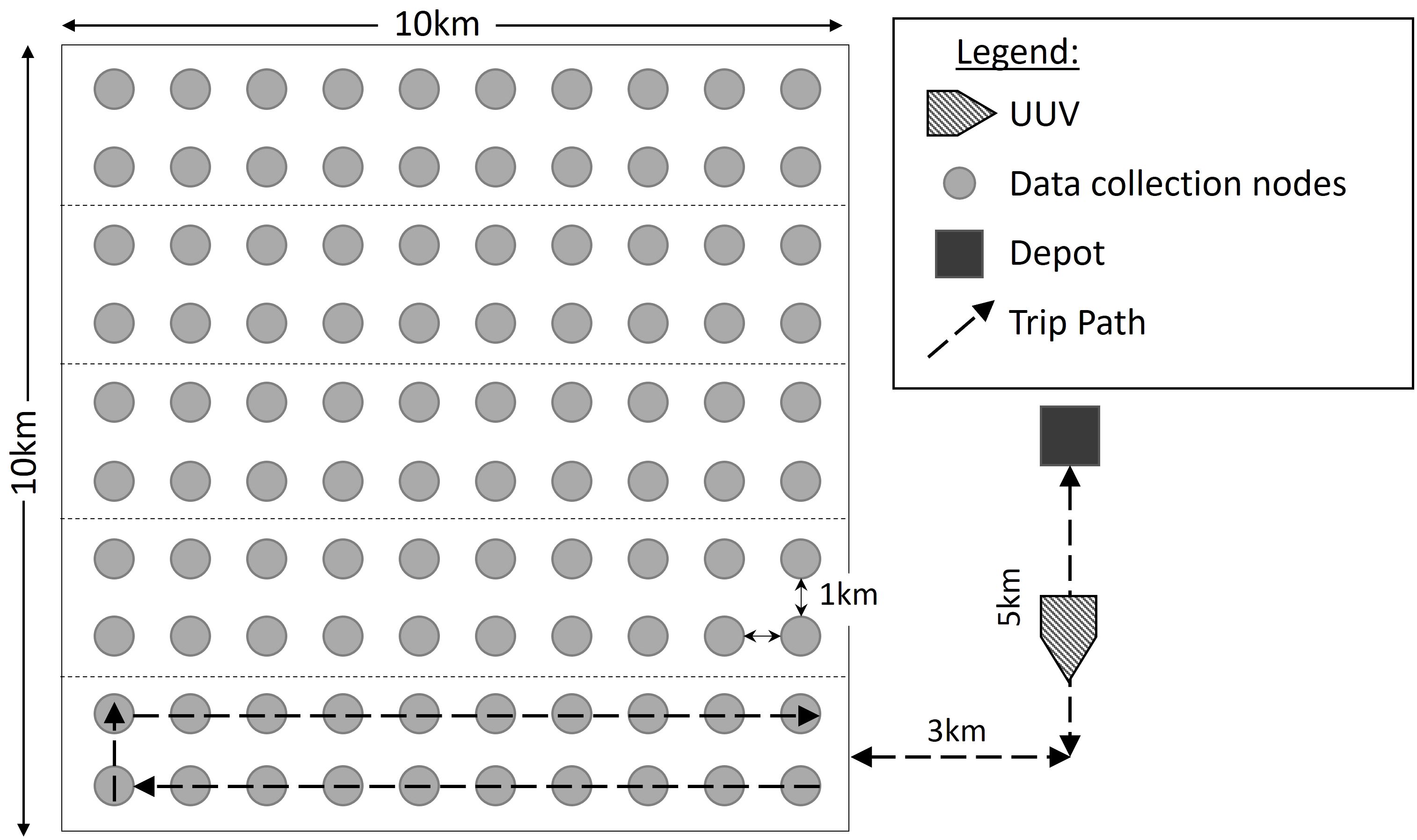
Figure 1 Data collection node layout with example city-block trip path. Figure originally published in Morey et al. (2021). Reprinted with permission from IEEE Proceedings of the 2021 Winter Simulation Conference.

Two distinct scenarios are considered in this paper that differ in how data are collected. Scenario 1 utilizes UUVs to collect a single data packet at each node location. The data packet is collected by the UUV and stored in the UUV until delivery to the depot. Scenario 2 utilizes stationary sensors as data collection nodes. These stationary sensors generate data continuously and store the data packets until a UUV arrives. Upon arrival of a UUV, all data packets generated since the arrival of a previous UUV, which is generally on the order of a thousand data packets, are transmitted to the UUV for storage and transportation to the depot. In both scenarios, the UUV ferries the data to the depot and recharges its battery while transmitting all data packets stored in the UUV to the depot. Scenario 1 could be thought of as a UUV surveying an area and collecting data, such as underwater mapping, as it travels. Scenario 2 could be thought of as a field of underwater sensors producing data, such as an environmental monitoring or surveillance application, where UUVs act as data ferries.

This research focuses on the topology design of UUVs to perform well in the above scenarios. Topology design, in this context, involves determining the configuration of assigning UUVs to visit data collection nodes. More specifically, this research aims to investigate two key questions: How many UUVs should be utilized in the configuration? How should UUVs be assigned to data collection nodes in clusters? This research inspects node/cluster revisit time, UUV failure rate, packet latency, and service distribution of UUVs to clusters as evaluation criteria. While cost is not directly measured in this analysis, as it is highly dependent on application specifics, the number of UUVs can be considered an indirect measure of cost, since UUVs are expensive and increased UUVs lead to increased miscellaneous costs, such as operational and maintenance costs.

To specify the topology design, we define a topology configuration by the number of UUVs, the assignment of UUVs to clusters, and the clustering of nodes. Table 1 contains a list of configurations considered in this paper, and Figure 2 demonstrates three example configurations. We let K represent the number of UUVs used in a configuration. We let N be the number of clusters. In the low-fidelity models, we assume five clusters consisting of 20 nodes each (i.e., N = 5). The high-fidelity simulation relaxes the assumption of fixed clusters to better represent a real-world implementation. Instead, clusters are based on predetermined routing, allowing for a layout with four clusters of 24 or 26 nodes each in two-UUV or four-UUV configurations (i.e., dividing the field into quadrants to more efficiently accommodate two or four UUVs). We let C be the number of clusters that each UUV visits, where 1 ≤ C ≤ N. By the assumption of workload balancing, C is the same for all UUVs in a configuration. For example, Figure 2A shows a configuration with K = 1, N = 5, and C = 5; Figure 2B shows a configuration with K = 2, N = 4, and C = 2; and Figure 2C shows a configuration with K = 2, N = 4, and C = 3. From the cluster perspective, we let k_i be the number of UUVs assigned to cluster i. The value of k_i is determined by the number of UUVs to assign, K; the total number of clusters, N; and the number of clusters assigned to each UUV, C. The values of K, C, and N are fixed for a configuration. We aim to have equal numbers of UUVs assigned to clusters, for load balancing, but some rounding is needed to obtain integer values of UUVs assigned to clusters. Therefore, the number of UUVs assigned to cluster i, k_i, is rounded to either the floor or the ceiling of $KC/N$ such that $\frac{1}{N}{\displaystyle {\sum }_{i=1}^N{k}_i=KC/N}$.

Table 1

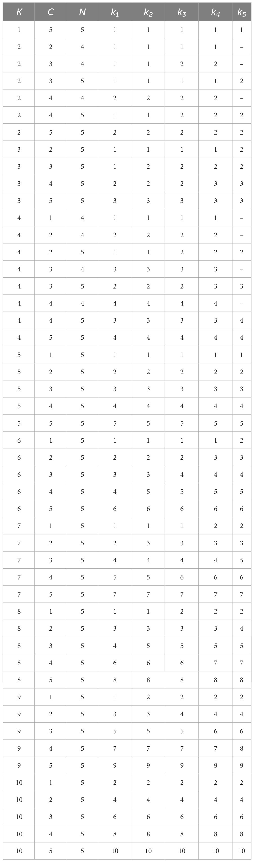
Table 1 List of topology design configurations with K UUVs, C clusters visited by each UUV, N total clusters in the configuration, and k_i UUVs assigned to cluster i.

Figure 2

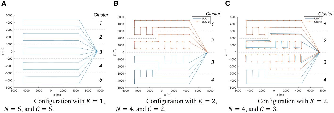
Figure 2 Example configurations with high-fidelity simulation routing. In (A) (left), a single UUV covers all clusters, visiting one cluster of 20 nodes per trip. In (B) (middle), four clusters of nodes are split evenly between two UUVs. In (C) (right), each UUV visits three clusters such that clusters 2 and 3 are visited by both UUVs. Figure originally published in Morey et al. (2021). Reprinted with permission from IEEE Proceedings of the 2021 Winter Simulation Conference.

The special case where C = N/K, which is when each cluster is serviced by exactly one UUV, is called a dedicated configuration. The special case where C = N, which is when every UUV visits every cluster, is called a full redundancy configuration. Table 1 shows the configurations evaluated for the low- and high-fidelity models. The low-fidelity models were run for the entirety of this finite decision space (i.e., each individual configuration). The insight gained from the low-fidelity models informed down-selection for high-fidelity simulation runs. While it is possible to run any of the configurations in the high-fidelity simulation, only selected configurations are presented in this paper.

Throughout the course of a mission, there is some chance that a UUV will fail and then must undergo repairs that take a finite amount of time. In a dedicated configuration, UUV failure causes no data to be collected from its assigned cluster(s) until the UUV is repaired. In a full redundancy configuration, clusters will continue to be serviced by other active UUVs in the event of UUV failure. A UUV is considered active if it is not in repair (i.e., servicing a cluster or charging).

Obtaining up-to-date information is often of critical importance in many mission scenarios. For this reason, we have identified average revisit time as a metric of interest, where revisit time is defined as the time elapsed between successive visits to a node by UUVs. By minimizing the revisit time, we ensure that the data collected are as timely as possible. Cost is another metric that is often important, but is highly uncertain. Instead of estimating cost directly, we consider the number of costly UUVs as a surrogate measure of cost. Another important metric of interest is the reliability of the system. To target reliability, we examine how UUV failures impact the proportion of time that UUVs are active and the resulting proportion of time each cluster of nodes is serviced.

3 Methods

Parameters that specify scenarios 1 and 2, which are inferred from the findings provided in a report as part of the study to support the Powering the Blue Economy Initiative by the U.S. Department of Energy (LiVecchi et al., 2019), are listed in Table 2. For modeling purposes, a UUV is assumed to travel at a constant speed and makes a round trip from the depot visiting data collection nodes without the risk of exhausting its battery. The UUV energy usage is comprised of travel energy usage, data collection energy usage at node locations, and data transmission energy usage to the depot. The UUV then delivers data to the depot via an optical link and recharges its battery at the depot.

Table 2

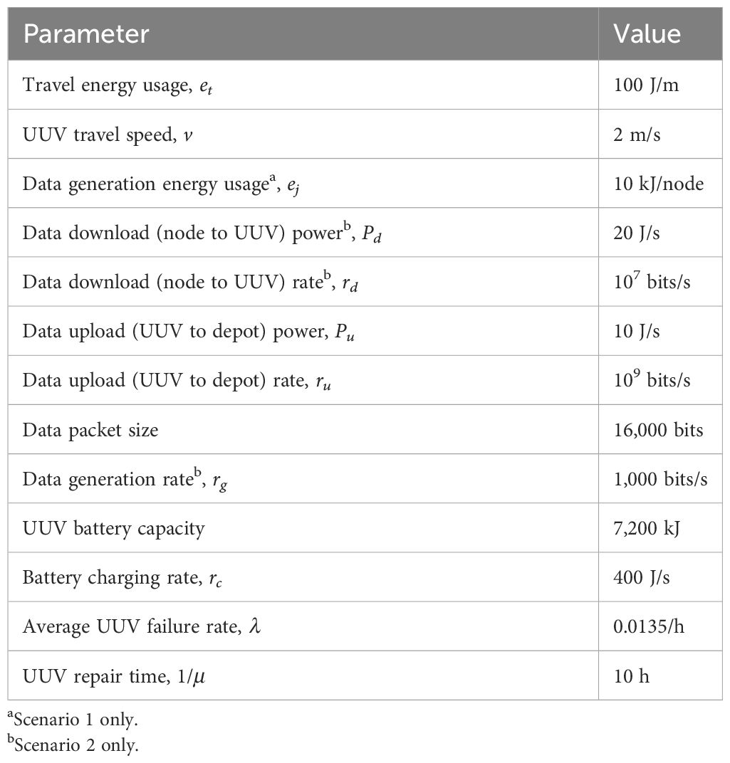
Table 2 Parameters for scenario specification.

3.1 Low-fidelity models

Three low-fidelity analytical models are developed to answer the two key questions. The first key question, regarding the number of UUVs, is examined using an average revisit time model. The second key question, regarding the assignment of UUVs to clusters, is examined using a queueing model and a utilization distribution model to characterize the service availability of UUVs for each cluster of nodes.

3.1.1 Average revisit time model

The revisit time for a node in a cluster is defined as the time between consecutive visits by any UUV. The average revisit time analytical model for a given configuration depends on the time it takes for a UUV to complete a trip in T seconds, which is given as

$\begin{array}{ll}T=\frac{d_t}{v}+\frac{e_t{d}_t+e_{ɡ}n}{r_c},& (1)\end{array}$

where d_t is the trip distance (meters), v is the UUV travel speed (m/s), e_t is the UUV travel energy (J/m), e_ɡ is the UUV energy required to gather data (J per node), n is the number of nodes per cluster (nodes), and r_c is the UUV battery charging rate (J/s). Values for v, e_t, and r_c are given in Table 2. Values for n and d_t are assumed to be fixed for the low-fidelity model, where the number of nodes per cluster is n = 20, and the trip distance is d_t = 3,600 m, which equals the worst-case city-block trip distance as illustrated in Figure 1. The value for e_g is scenario-dependent. Data are uploaded from the UUV to the depot concurrently with UUV charging, and the energy consumption to do so is negligible compared with the travel energy usage. Notice that the dominant term contributing to the trip time in Equation 1 is the travel time, d_t/v, with the parameters in Table 2.

Revisit time, $R_{k_i,C}$, for a node in cluster i with a trip time of T hours from Equation 1 is

$\begin{array}{ll}{R}_{k_i,C}=T\frac{C}{k_i}=\left(\frac{d_t}{v}+\frac{e_t{d}_t+e_{ɡ}n}{r_c}\right)\frac{C}{k_i}.& (2)\end{array}$

The UUV energy required to gather data per trip in Equation 2, e_g, depends on the scenario. For scenario 1 where there is a single data packet generated at each data collection node by the UUV, the data gather energy equals the data generation energy usage, i.e., e_g = e_j from Table 2. The revisit time, $R_{k_i,C}$, for scenario 1 of a node in cluster i is

$\begin{array}{ll}\text{Scenario} 1:R_{k_i,C}=\left(\frac{d_t}{v}+\frac{e_t{d}_t+e_{j}n}{r_c}\right)\frac{C}{k_i}.& (3)\end{array}$

For scenario 2, the energy required to gather data per trip, e_g, is a function of the revisit time, $R_{k_i,C}$, and is $e_g=R_{k_i,C}(r_g{p}_d/r_d)$, where r_g is the data generation rate at each node (bits/s), p_d is the power required to download data from a data collection node to the UUV (J/s), and r_d is the data download rate from a data collection node to the UUV (bits/s), with values given in Table 2. Manipulating Equation 2 with the expression for e_g, we solve for $R_{k_i,C}$ which yields the revisit time for scenario 2, as

$\begin{array}{ll}\text{Scenario} 2:R_{k_i,C}=\frac{C{r}_d{d}_t(r_c+e_{t}v)}{v(k_i{r}_c{r}_d-C{r}_{ɡ}{p}_{d}n)}.& (4)\end{array}$

Given $R_{k_i,C}$ in Equation 3 for scenario 1 and Equation 4 for scenario 2, the average revisit time across all N clusters is

$\begin{array}{ll}{\tilde{R}}_{K,C}=\frac{1}{N}\sum _{i=1}^N{R}_{k_i,C}.& (5)\end{array}$

3.1.2 UUV service availability queueing model

Given a configuration with K UUVs, it is beneficial to understand the proportion of time those UUVs are active rather than in repair. This is determined via a finite population queueing model of population size K (Gross and Harris, 1998).

The finite population queueing model consists of K UUVs as customers that enter the repair system when they break down and leave the system when they are repaired. The servers repair the UUVs and we assume there are at least as many servers as UUVs so that there are enough resources for UUVs to be repaired in parallel. Assume the average UUV failure rate is λ per hour and the repair rate is µ per hour (see Table 2). The state of the repair system is the number of UUVs currently in repair. The steady-state probability of i UUVs being in repair, P_i, is

$P_i=\{\begin{array}{cc}\frac{1}{{\sum }_{n=0}^K\frac{K!}{(K-n)!n!}{(\frac{\lambda }{\mu })}^n}& \text{ for }i=0\\ \frac{K!}{(K-i)!i!}{(\frac{\lambda }{\mu })}^i{P}_0& \text{ for }i=1,\dots ,K.\end{array}$

The values of P_i for K = 5 are shown in Figure 3.

Figure 3

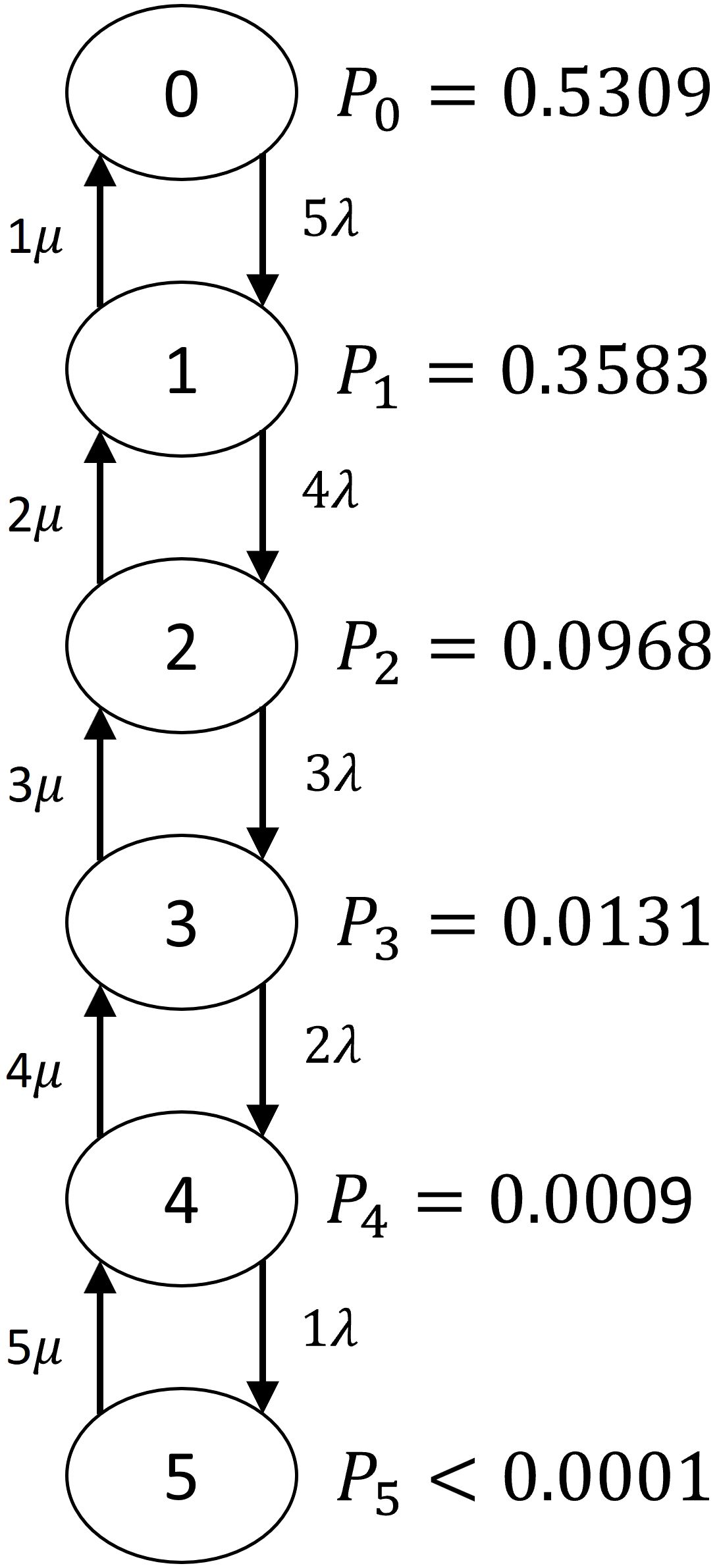
Figure 3 UUV service availability queueing model for K = 5 with λ = 0.0135 and µ = 0.1.

3.1.3 Utilization distribution model

To determine the optimal method of assigning UUVs to clusters with a given number of UUVs, a utilization distribution model is developed. This analysis focuses on two configurations: dedicated and full redundancy. A dedicated configuration is one in which each UUV visits a unique set of clusters. From the cluster perspective, a dedicated configuration can be characterized by each cluster being visited by a single UUV. A full redundancy configuration, on the other hand, has each UUV visiting every cluster.

In order to distinguish dedicated and full redundancy configurations, we must consider the situations in which some UUVs are in repair. In the case of a dedicated configuration, any cluster assigned to a UUV that is in repair is not serviced for the entire time that the UUV is in repair and all the other clusters are unaffected. In the case of full redundancy, all clusters are assigned to all UUVs. Thus, active UUVs service all clusters, effectively distributing the detriment of the loss of a UUV between all clusters. One way to visualize the difference between these two configurations is in the proportion of time a cluster has an active UUV assigned to it.

The dedicated configuration can be considered an all-or-nothing configuration. For every UUV in repair, its assigned cluster(s) will spend 0% of the time being served, while all the other clusters spend $100\frac{C}{K}\%$ of the time being served, where C is the total number of clusters in the configuration and K is the total number of UUVs. For a dedicated configuration, the percent of time that cluster i spends with its assigned UUV active, $P_i^{\text{ded}}$, is given as

$\begin{array}{ll}{P}_i^{\text{ded}}=\{\begin{array}{cc}100\frac{C}{K}\%& \text{for active UUV}\\ 0\%& \text{for UUV in repair}.\end{array}& (6)\end{array}$

The full redundancy configuration is a more balanced configuration. All clusters will split the detriment of having a UUV in repair evenly. For a full redundancy configuration, the percentage of time that cluster i spends with its assigned UUV active, $P_i^{\text{red}}$, is given as

$\begin{array}{ll}{P}_i^{\text{red}}=\frac{C}{u}\%& (7)\end{array}$

where u is the number of currently active UUVs.

3.2 High-fidelity simulation

The high-fidelity model simulates a detailed scenario with specific data collection node locations, UUV routes, schedules, energy usage, and data transfer over specified communication links. Unlike the low-fidelity models where UUV routing is modeled by their assignment to clusters with a fixed trip time, the high-fidelity simulation predefines specific routing for each trip that a UUV takes, as shown in Figure 2. A waypoint mobility model is used to define UUV movement along this predefined path and a UUV is considered to have arrived at a node once it comes within a 25-m radius of the node. Departures of UUVs from the depot are staggered at the start of the simulation to avoid packet collisions when uploading to the depot. To enforce load balancing, a departing UUV is scheduled to visit the assigned cluster that was least recently visited by a UUV.

Throughout the simulation, a battery model is used to track the energy remaining in the UUV as it travels. Energy usage leverages a built-in modem energy model that accounts for the power usage during communication events to subtract energy from the UUV’s battery. The UUV recharges at the depot until its battery is full. Parameter values are shown in Table 2.

UUV failures occur at randomly drawn times during a trip based on a prespecified probability that is consistent with the failure rate, λ, in Table 2. Packets already stored in the UUV are lost with each UUV failure. In scenario 2, packets in the clusters not yet collected remain at sensor nodes for the next UUV to arrive. Failed UUVs remain at the depot for a prespecified repair time.

The high-fidelity communication simulation model is developed using the Network Simulator NS3 (NS-3 Consortium, 2021) and utilizes the underwater acoustic network (UAN) module, as future research aims to expand the use of acoustic communications. For simplicity and rapid development, the models available within the UAN are leveraged for all links. The communications link between the UUV and the depot is a fiber-optic link available when the UUV docks physically to the depot. The properties of the link are approximated by setting the carrier frequency to 1 MHz and the data rate to 1 GHz. The sensor-to-UUV communications link in scenario 2 represents a free-space optical (FSO) link. Similarly, because no FSO model exists in NS3, the acoustic propagation models in the UAN module of NS3 are used with a high center frequency (30 kHz) and configured with a data rate of 10 Mbps to approximate an FSO link. Data upload and download rates for fiber-optic and FSO links are specified in Table 2.

There are many additional considerations and parameters that could be added and investigated in future studies but have thus far been omitted from the high-fidelity simulation for tractability. A partial list includes water currents inducing UUV drift, navigation variance due to inertial navigation error, failures at the depot preventing recharging of all UUVs/slow charging/etc., limitations on the number of UUVs that can recharge at a time, sea state impacting the ability to recover a UUV for repair/service at a given time, dynamic UUV path planning, logic for UUVs to return to the depot based on actual energy usage (varying due to currents, battery health, etc.) instead of assumed constant energy usage rate, and varying repair time based on specific UUV failure modes.

The high-fidelity simulation model tracks a variety of metrics, including UUV trip times (time elapsed between a UUV’s departure from the depot and that UUV’s next departure from the depot), node revisit times (time elapsed at a node between two visits by any UUV), individual data packet latencies (time elapsed between data packet generation and delivery to the depot), and data age of a cluster (time elapsed between delivery to the depot from a cluster until the next delivery from the same cluster). The simulation provides highly accurate results but requires a high computation cost. Thus, we perform high-fidelity simulation evaluations only for selected topology configurations based on the results of the low-fidelity models. We use common random seeds to compare configurations.

4 Results

We consider the results with respect to two different scenarios. Scenario 1 is a scenario in which a single data packet is collected at each data collection node. Each UUV is equipped with a sensor (such as a sonar system) for data collection. The UUV travels to each data collection node, which is a location to be visited rather than a physical node, to collect sensor data at that location. Scenario 2 is a scenario in which data are being generated continuously and stored at data collection nodes until a UUV arrives to download and transport the data. When a UUV arrives, the data generated since the last UUV visit are discretized into an integer number of data packets and retrieved by the UUV.

Because scenario 1 only transmits one data packet per visit and thus only requires 10−15 s to run the high-fidelity simulation via NS3 (NS-3 Consortium, 2021) on a Dell Precision 7720 with 2.9 GHz i7 processor and 32 GB RAM (i.e., a standard laptop), it is tractable to perform 20 Monte Carlo replications and average the metrics of interest. In scenario 2, on the other hand, thousands of data packets are generated and transmitted per UUV visit at each node. Each data packet transmission is modeled individually, causing the computation time to be approximately 3 h for a single simulation run. Monte Carlo replications are impractical and so metrics are recorded only for a single simulation run. The low-fidelity simulations are coded in Excel and Python and take less than a millisecond to run on an ROG Zephyrus G14 with an AMD Ryzen 9 4900HS processor and 24 GB RAM (i.e., a standard laptop).

In both scenario 1 and scenario 2, we first aim to determine how many UUVs should be utilized in the configuration and then how clusters should be assigned to those UUVs.

4.1 How many UUVs?

To determine how many UUVs should be utilized in a configuration for scenario 1, we first examine how the number of UUVs impacts the average revisit time. The parameters in Table 2 are used in the low-fidelity average revisit time model in Equations 3, 5. The averages across configurations with the same number of UUVs are plotted in Figure 4A as circles. Additionally, the lowest average revisit time calculated for each number of UUVs from the low-fidelity average revisit time model is detailed in Table 3A along with the improvement relative to the single UUV case as well as relative to the case with one fewer UUV.

Figure 4

Figure 4 Revisit time results. (A) Scenario 1. (B) Scenario 2.

Table 3

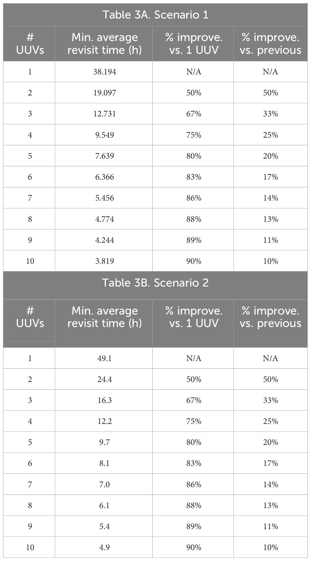
Table 3 Low-fidelity average revisit times.

High-fidelity simulation runs were performed for up to five UUVs since additional UUVs showed very little improvement in average revisit time. The high-fidelity simulation reports the revisit time experienced by each node in the simulation for each time the node is visited. The average revisit time is calculated by averaging all individual revisit times observed over the course of the 20 Monte Carlo runs for one configuration. The average across all configurations with the same number of UUVs is plotted in Figure 4A as squares. The large spread between the minimum and maximum revisit times, also shown in Figure 4A, demonstrates the variability in revisit times due to UUV failures.

The average revisit time metric for both the high- and low-fidelity models (Figure 4A) shows that more UUVs yield lower revisit times, which is beneficial in most mission contexts. However, the incremental improvement of each added UUV decreases. This provides a trade-off between the number of costly UUVs and the decrease in revisit time. Note that the high- and low-fidelity models produce consistent trends. From the average revisit time versus the number of UUVs’ trade-off curves, configurations with five UUVs are selected as a baseline solution for further analysis because each additional UUV results in less than a 20% improvement, as in Table 3A.

To explore the sensitivity of the number of active UUVs to UUV failure rate, we run the low-fidelity UUV service availability queueing model by varying the average time to failure, 1/λ, for 1,000 discrete values varying from 0 to 150 h for five UUVs and all other parameter values fixed at the values in Table 2. The results are presented in Figure 5. This figure shows, for example, that if each UUV fails every 70 h on average, then all five UUVs will be active 51% of the time, exactly four UUVs will be active 37% of the time, and four or more UUVs will be active 88% of the time.

Figure 5

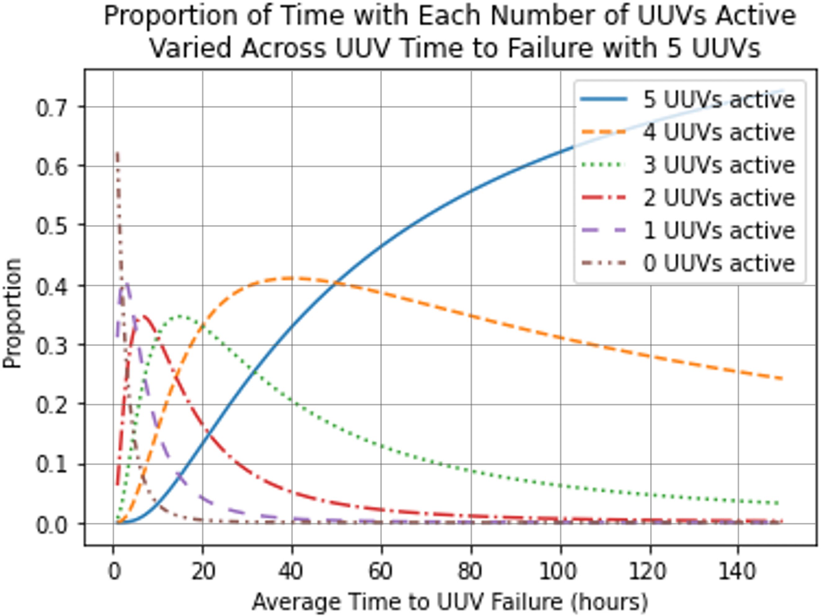
Figure 5 Sensitivity to UUV failure rate for five UUVs.

The low-fidelity average revisit time model for scenario 2 produces very similar results to those from scenario 1. The average revisit time, as given in Equation 4 and Equation 5, is averaged across configurations for the same number of UUVs and plotted in Figure 4B as circles. The lowest average revisit time for each number of UUVs and the incremental improvement from the low-fidelity average revisit time model are detailed in Table 3B. Similar to scenario 1, the incremental improvement decreases with each additional UUV.

The high-fidelity simulation reports the average of all individual node revisit times over a single simulation replication. The average across all configurations with the same number of UUVs is plotted in Figure 4B as squares. The high-fidelity simulation shows consistent trends with the low-fidelity average revisit time model. The complexity of scenario 2, however, leads to a larger difference between the average revisit time calculated by the high-fidelity simulation and the low-fidelity model (see Figure 4B). Consistent with the low-fidelity model, the high-fidelity simulation demonstrates that increasing the number of UUVs in a configuration decreases the average revisit time with decreasing incremental improvement.

Notice that the UUV service availability queueing model does not differentiate between scenario 1 and scenario 2. As such, the same results drawn from the model in scenario 1, as shown in Figure 5, apply to scenario 2.

Both scenarios elicit very similar revisit time results and, subsequently, lead to the same insight as to the number of UUVs to include in a configuration. The increased data packages in scenario 2, which take time and energy to transmit, lead to increased revisit times in comparison to scenario 1 but do not affect the overall trends in how the number of UUVs impacts the average revisit time. To summarize, an increased number of UUVs leads to lower average revisit times with decreased incremental improvement regardless of the scenario.

4.2 How to assign UUVs to clusters?

Once a number of UUVs, K, has been selected, we must determine how many clusters each UUV will visit. In order to more easily quantify the assignment of UUVs to clusters, we introduce the measure of coverage, which is defined as K ∗ C ∗ 100 and represented as a percentage. For this analysis, we consider only coverages of at least 100%, which merely ensures that all clusters are serviced. Higher percentage coverage indicates increased redundancy, or in other words, multiple UUVs servicing the same clusters.

First, we examine scenario 1. Figure 6 shows the average and variance revisit times observed by the high-fidelity simulation for different numbers of UUVs as a function of coverage. Each individual revisit time observed within a simulation run is used to calculate the average and variance, and then these metrics are averaged over the 20 Monte Carlo replications. The average revisit time indicates no impact due to coverage, while variance decreases with increased coverage.

Figure 6

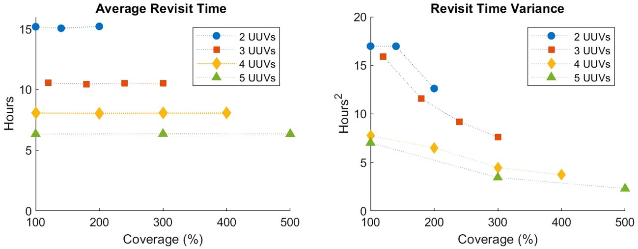
Figure 6 High-fidelity average and variance of revisit times for scenario 1 averaged over 20 Monte Carlo runs.

To interpret what this change in variance means, we examine the packet- and node-level data collected by the high-fidelity simulation. Figures 7A, B show histograms of revisit times observed for two different configurations of five UUVs. In Figure 7A, for a dedicated configuration, large revisit times of greater than 12 h are more frequently observed. In Figure 7B, for a full redundancy configuration, there are fewer revisit times of greater than 12 h and, overall, more evenly spread observations.

Figure 7

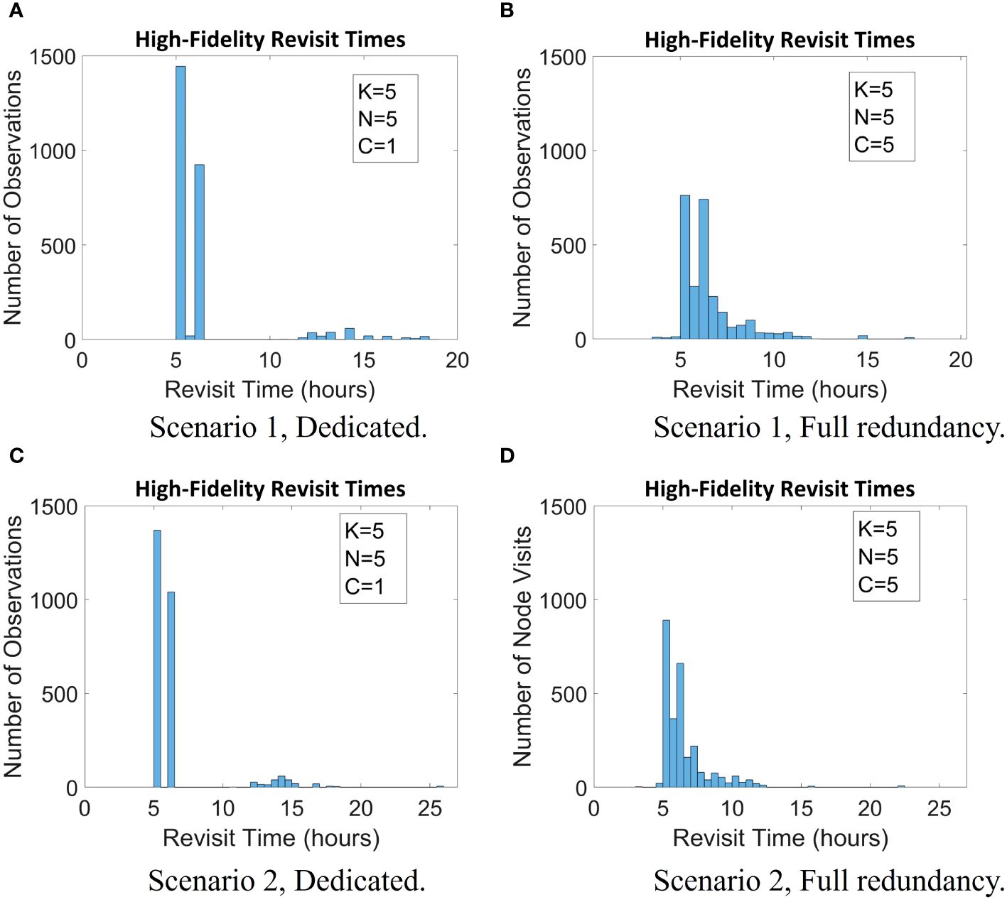
Figure 7 Histogram of revisit times for two configurations generated by the high-fidelity simulation for both scenarios 1 and 2. (A) Scenario 1, dedicate; (B) Scenario 1, Full redundancy; (C) Scenario 2, dedicate; (D) Scenario 2, Full redundancy.

For further insight into how coverage impacts the performance of a configuration, we use the low-fidelity models in conjunction with the high-fidelity results. The low-fidelity utilization distribution model defined by Equation 6 and Equation 7, which is used to distinguish between dedicated and full redundancy configurations, requires a fixed value for K. We select K = 5 UUVs because the improvement in revisit time beyond five UUVs is small (see Figures 4A, B). Notice that these equations do not depend on any data collection parameters. Rather, this low-fidelity model provides cluster-level metrics that do not vary between scenario 1 and scenario 2. Example results of the low-fidelity utilization distribution model for four of five UUVs and two of five UUVs being active are presented in Table 4.

Table 4

Table 4 Percent of time clusters having an active UUV with four or two of five UUV's active, with averages listed in bold.

As can be seen in Table 4, the average percent of time spent with an active UUV assigned to it across all clusters (the column average) is equivalent to dedicated and full redundancy configurations. The difference, then, can be seen in how the time spent with an active UUV assigned to it is distributed among each of the clusters, where full redundancy is more balanced than dedicated.

Additional detailed metrics such as UUV trip times, node revisit times, data packet latencies, and data age of a cluster are also gathered by the high-fidelity simulation. For example, the data age is analyzed and indicates that the most common data age is equal to the trip time of approximately 5 h. There are also several unusually high data ages observed due to UUV failures, which become less extreme as coverage increases.

Figures 7C, D plot the high-fidelity revisit times observed for two different configurations of five UUVs for scenario 2. Similar to the results for scenario 1, there are several observed larger revisit times for the dedicated configuration (Figure 7C), and a tighter clustering of revisit times is observed for the full redundancy configuration (Figure 7D).

The node-level average and variance of revisit times for two, three, and five UUVs are shown in Figure 8A for scenario 2. In contrast to scenario 1, where the results are averaged over Monte Carlo runs, these results are extracted from revisit times observed over a single replication of the simulation. We observe a decrease in the variance of revisit time as coverage increases except in the case of two UUV configurations and no impact on average revisit time from coverage.

Figure 8

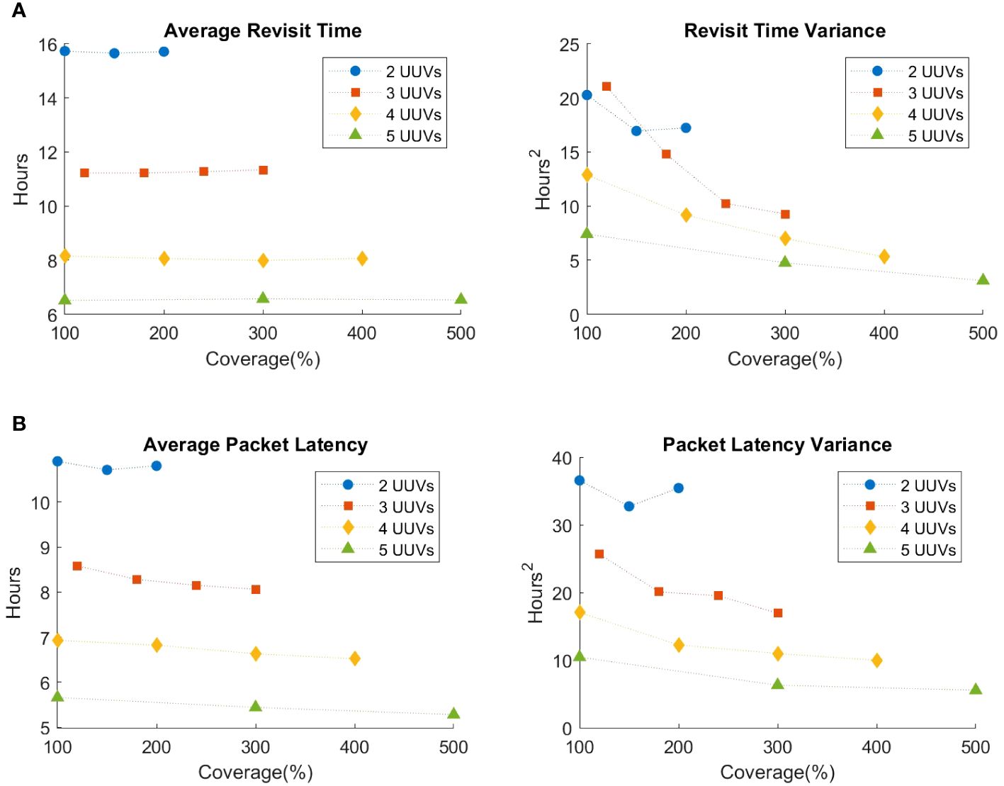
Figure 8 High-fidelity aggregate results for scenario 2 for a single run. (A) High-fidelity aggregate revisit time results for scenario 2. (B) High-fidelity aggregate packet latency results for scenario 2.

With the continuous generation of data packets in scenario 2, as opposed to a single packet collected per UUV visit in scenario 1, the high-fidelity simulation is additionally able to collect packet-level metrics, such as individual packet latencies, that further demonstrate the impact of UUV failures. Packet-level average and variance of latency are plotted in Figure 8B. Packet-level average and variance of latency also decrease as coverage increases except in the case of two UUV configurations. The inconsistent increase observed in Figures 8A, B in the case of two UUVs may be due to results obtained from only a single replication.

Figure 9 shows the individual packet latencies observed by the high-fidelity simulation for a dedicated configuration and a full redundancy configuration. The dedicated configuration (Figure 9A) shows several extremely high observed latencies (over 15 h), which are the effect of clusters not getting visited for a long period of time due to their assigned UUV failing. The full redundancy configuration (Figure 9B) shows slightly higher latencies (between 10 and 15 h) but very few extremely high latencies (over 15 h). This indicates that, while more clusters (and, subsequently, more individual packets) are impacted by UUV failure, the magnitude of the impact is lessened.

Figure 9

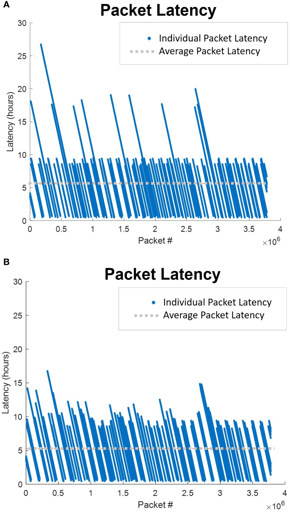
Figure 9 Individual pack latencies for two configurations with five UUVs generated by the high-fidelity simulation for scenario 2. (A) Dedicated; (B) Full Redundancy.

Overall, the results from scenario 1 and scenario 2 have the same general trends. While the assignment of UUVs to clusters does not directly influence key metrics such as the average revisit time, it does impact how UUV failures affect the configuration. More specifically, dedicated configurations isolate the impact of UUV failures, while full redundancy configurations distribute the impact. Due to the high computational expense of the scenario 2 high-fidelity simulation and the subsequent intractability to perform Monte Carlo replications, scenario 2 intuitions rely even more heavily on the low-fidelity models. The analysis at this time does not dive deeper into the subtle differences between scenarios 1 and 2, but future work could examine them jointly in terms of the optimal use of UUVs as sensors versus data ferries.

5 Discussion

Although scenarios 1 and 2 have some important differences in their structure, aggregate trends remain consistent for both. In both scenarios, there is a trade-off between the number of costly UUVs and the improved revisit times observed with a greater number of UUVs. The low-fidelity average revisit time model estimates the improvement in revisit time for a wide range of possible UUV counts. Decision makers can use high-fidelity simulation to gain a deeper and more accurate understanding of the most promising cases. Without mission-specific knowledge, such as timeliness requirements, priority of data collection clusters, and maximum UUV budget, we cannot make an exact claim as to the optimal number of UUVs. Rather, we provide insight into the trends and trade-offs.

Due to the possibility of UUV failure, every UUV in a configuration may not be operational at all times. The low-fidelity UUV service availability queueing model provides the proportion of time each UUV is active. For applications where revisit time guarantees are critical, it may be beneficial to have additional UUVs in the configuration. For example, consider scenario 2 and suppose that revisit times of less than 10 h are desirable, which occurs when there are five or more UUVs (see Figure 4B). Figure 5 shows that, with five UUVs in the configuration, the proportion of time that all five UUVs are active is only 53% of the time. Alternatively, with six UUVs in the configuration, the proportion of time that at least five UUVs are active is 95%. In such situations, for example, decision makers may determine that the cost of a sixth UUV is worthwhile to ensure five UUVs are operational at a higher proportion of time.

The low-fidelity UUV service availability queueing model can also be used to understand the impact of time to failure on the number of active UUVs. Suppose that the average time to repair a UUV is fixed at 10 h and a maximum UUV budget of five UUVs, but it is possible to alter the average time until UUV failure. If we want to ensure that all five UUVs will be operational at least 60% of the time, then based on Figure 5, it would need to be ensured that the UUVs fail no more frequently than once every 90 h. Other sensitivity analyses are also possible due to the analytic nature of the three low-fidelity models.

With a selected number of UUVs, the amount of coverage must be determined, where one extreme is a dedicated configuration (each cluster visited by a single UUV) and the other is full redundancy (all clusters visited by all UUVs). The low-fidelity utilization distribution model demonstrates how dedicated configurations isolate the impact of failed UUVs, whereas full redundancy configurations distribute the impact. Detailed metrics gathered by the high-fidelity simulation, such as node-level revisit interval and packet-level latency, support this observation.

Determining whether a dedicated configuration or a full redundancy configuration is preferable is mission-dependent. For example, consider a mission where data quickly become outdated and unusable. In this mission, a dedicated configuration would be preferable because UUV failure would only impact the data latency of a few clusters (whereas a full redundancy configuration would increase the latency of all clusters, making all the data useless). Now consider a different mission where having at least some data from all clusters at all times is critical. In this case, a full redundancy configuration would be ideal as it would ensure all clusters are being serviced as long as there is even a single active UUV.

There may be missions where timely delivery of data from some clusters is more critical than others. The findings in this paper lend themselves to a dynamic solution to this problem. For example, if one cluster is highly prioritized while the others are equally prioritized, UUVs can be dynamically assigned such that the high-priority cluster is always assigned a dedicated active UUV (if one exists) and all the other clusters share any remaining UUVs. In another example where each cluster has a different priority, UUVs can be dynamically assigned such that any active UUVs are assigned to the highest priority clusters in order and any remaining lower priority clusters are not visited.

Considerations when selecting a configuration for a mission include the importance/priority of clusters, emphasis on timeliness of data and/or variety of data, and differences between trip times to visit clusters.

6 Conclusion

Military applications have long been at the forefront of advancements in operations research. With advancements in technology come advancements in modeling techniques. One such example is the rising use of unmanned vehicles, especially in maritime environments where communications are limited. The complex systems prevalent in military applications require sophisticated modeling methods, but these models often come at the price of high computational cost. Simplified or low-fidelity models, on the other hand, reduce computational cost at the expense of accuracy.

This paper uses a multifidelity approach to analyze the trade-offs posed by different potential topology design configurations, where a configuration is defined by the number of UUVs in use (K), the number of data collection node clusters (N), and the number of clusters that each UUV services (C). We contribute to prior work through the consideration of UUV failures, the exploration of a continuous data collection scenario (scenario 2), the development of additional low-fidelity models, and the analysis of differing configurations with the same number of UUVs. Since requirements and priorities vary from application to application, the configuration that is considered optimal is application-dependent and subjective. In this way, both the low-fidelity analytical models and the high-fidelity simulation are necessary to make informed decisions. The low-fidelity models analyze aggregate-level metrics for a wide array of parameters to help determine the most promising configurations, while the high-fidelity simulation provides details for those promising configurations that are important for informed decisions.

In future work, we aim to explore topology configuration designs for scenarios with time-sensitive underwater communication and networking applications to support situational awareness and command and control capabilities. We will consider the density and placement of communication relay nodes and network control nodes and the number and routing patterns of UUVs in the topology configurations. Furthermore, additional metrics of interest, such as application-specific economic analysis or multiple communication modalities and data rates, can be considered in future work. Additionally, we will incorporate information-centric networking architectures (Jacobson et al., 2009; Burke et al., 2018) in our models to evaluate emerging and promising networking technologies that could be of great importance to future distributed maritime operations.

Data availability statement

The original contributions presented in the study are included in the article/supplementary material. Further inquiries can be directed to the corresponding author.

Author contributions

DM: Writing – review & editing, Writing – original draft, Software, Formal analysis, Conceptualization. RP: Writing – review & editing, Software, Formal analysis, Conceptualization. CW: Writing – review & editing, Funding acquisition, Formal analysis, Conceptualization. ZZ: Writing – review & editing, Supervision, Funding acquisition, Formal analysis, Conceptualization.

Funding

The author(s) declare financial support was received for the research, authorship, and/or publication of this article. This work has been supported in part by the Office of Naval Research (ONR), award number N00014-23-1-2359, and the Naval Information Warfare Center Pacific.

Conflict of interest

The authors declare that the research was conducted in the absence of any commercial or financial relationships that could be construed as a potential conflict of interest.

Publisher’s note

All claims expressed in this article are solely those of the authors and do not necessarily represent those of their affiliated organizations, or those of the publisher, the editors and the reviewers. Any product that may be evaluated in this article, or claim that may be made by its manufacturer, is not guaranteed or endorsed by the publisher.

References

Burke J., Afanasyev A., Refaei T., Zhang L. (2018). “NDN impact on tactical application development,” in 2018 IEEE Military Communications Conference, Los Angeles, CA. 640–646. doi: 10.1109/MILCOM.2018.8599725

CrossRef Full Text | Google Scholar

Button R. W., Kamp J., Curtin T. B., Dryden J. (2009). A survey of missions for unmanned undersea vehicles (Santa Monica, CA: RAND Corporation).

Google Scholar

Cho P. C., Batta R. (2021). “UAV search path optimization for recording emerging targets”. Military Operat Res. 26, 27–48. doi: 10.5711/1082598326327

CrossRef Full Text | Google Scholar

Fletcher B. (2000). “UUV master plan: a vision for Navy UUV development,” in Proceedings of the OCEANS 2000 MTS/IEEE Conference and Exhibition (IEEE Conference Comittee), Piscataway, NJ. 65–71. doi: 10.1109/OCEANS.2000.881235

CrossRef Full Text | Google Scholar

Fu M. C. (2015). Handbook of simulation optimization (New York, NY: Springer).

Google Scholar

Garau B., Alvarez A., Oliver G. (2005). “Path planning of autonomous underwater vehicles in current fields with complex spatial variability: an A* approach,” in Proceedings of the 2005 IEEE International Conference on Robotics and Automation, Barcelona, Spain. 194–198 (IEEE).

Google Scholar

Gosavi A. (2015). Simulation-based optimization. 2nd ed. (New York: Springer). doi: 10.1007/978-1-4899-7491-4

CrossRef Full Text | Google Scholar

Gross D., Harris C. M. (1998). Fundamentals of queueing theory. 3rd ed. (New York: Wiley-Interscience).

Google Scholar

Huang H., Zabinsky Z. B. (2014). “Multiple objective probabilistic branch and bound for pareto optimal approximation,” in Proceeding of the 2014 Winter Simulation Conference (Institute of Electrical and Electronics Engineers Inc.), 3916–3927. doi: 10.1109/WSC.2014.7020217

CrossRef Full Text | Google Scholar

Jacobson V., Smetters D. K., Thornton J. D., Plass M. F., Briggs N. H., Braynard R. L. (2009). “Networking named content.” In CoNEXT ^′09: Proceedings of the 5th International Conference on Emerging Networking Experiments and Technologies (New York, NY: Association for Computing Machinery), 1–12. doi: 10.1145/1658939

CrossRef Full Text | Google Scholar

LiVecchi A., Copping A., Jenne D., Gorton A., Preus R., Gill G., et al. (2019). “Powering the Blue Economy; exploring Opportunities for Marine Renewable Energy in Maritime market.” (Washington, D.C: U.S. Department of Energy, Office of Energy Efficiency and Renewable Energy).

Google Scholar

Mete H. O., Zabinsky Z. B. (2014). “Multiobjective interacting particle algorithm for global optimization.” INFORMS J. Computing 26, 500–513. doi: 10.1287/ijoc.2013.0580

CrossRef Full Text | Google Scholar

Morey D. F., Zabinsky Z. B., Wakayama C., Plate R. (2021). “Multi-fidelity modeling for the design of a maritime environmental survey network utilizing unmanned underwater vehicles,” in Proceedings of the Winter Simulation Conference. 1–12 (IEEE Press). doi: 10.1109/WSC52266.2021.9715365

CrossRef Full Text | Google Scholar

NS-3 Consortium (2021) Network simulator NS-3 consortium (Accessed Feb. 15, 2021).

Google Scholar

Soulignac M., Taillibert P., Rueher M. (2009). “Time-minimal path planning in dynamic current fields,” in Proceedings of the 2005 IEEE International Conference on Robotics and Automation. 2473–2479.

Google Scholar

Vasilescu I., Kotay K., Rus D., Dunbabin M., Corke P. (2005). “Data collection, storage, and retrieval with an underwater sensor network,” in Proceedings of the 3rd International Conference on Embedded Networked Sensor Systems, New York, New York. 154–165 (Association for Computing Machinery). doi: 10.1145/1098918.1098936

CrossRef Full Text | Google Scholar

Witt J., Dunbabin M. (2008). “Go with the flow: Optimal AUV path planning in coastal environments,” in Proceedings of the 2008 Australasian Conference on Robotics and Automation, Canberra, Australia. 1–9.

Google Scholar

Zwolak K., Simpson B., Anderson B., Bazhenova E., Falconer R., Kearns T., et al. (2017). “An unmanned seafloor mapping system: The concept of an AUV integrated with the newly designed USV SEAKIT,” in Proceedings of OCEANS 2017 - Aberdeen, Aberdeen, UK. 1–6.

Google Scholar