Variability in coastal habitat available for Longfin Smelt Spirinchus thaleichthys in the northeastern Pacific Ocean

1 Introduction

Oceanographic conditions and processes, especially those related to natural climate variability and global climate change, are well known drivers of marine animal distribution and population dynamics (Murawski, 1993; Mantua et al., 1997; Cavole et al., 2016). Understanding how these conditions and processes affect species of management concern is fundamental to the development of effective management strategies. Longfin Smelt (Spirinchus thaleichthys) is an anadromous, schooling, forage fish found in coastal waters along the Pacific coast of North America from central California to Alaska. Adults reproduce in fresh and brackish regions of estuaries, with larval fish rearing in the estuary prior to emigrating to the ocean (Merz et al., 2013). Timing of these life history events is uncertain range-wide but presumably varies with latitude. In California, most reproduction likely occurs from December to April. Emigration to the ocean is largely completed by the end of their first year of life, but some individuals may stay in large estuaries year-round (Bottom et al., 1984; Merz et al., 2013). Longfin Smelt return to the estuaries and move into spawning habitats from November to January of their second year (Moyle, 2002; Merz et al., 2013). This complex life history makes Longfin Smelt vulnerable to threats in freshwater and at sea.

Substantial long-term declines (~99%) of the southern-most reproducing population (Sommer et al., 2007) have led to Longfin Smelt being listed as a threatened species under the California Endangered Species Act (California Fish and Game Commission, 2009), protection in the state of Oregon (Oregon state rule OAR 635-004-0545), and it is currently a candidate species for protection under the United States Endangered Species Act (U.S. Fish and Wildlife Service, 2023). Understanding drivers of Longfin Smelt population trends is highly management relevant as critical freshwater habitat used for spawning and rearing is a key component of the state of California’s water supply. Water is extracted from the upper San Francisco Estuary to supply municipal water needs for millions of people in central and southern California and a multi-billion-dollar agricultural industry in California’s Central Valley (Lund, 2016). The amount of water that can be withdrawn from the ecosystem is regulated, in part, to protect at-risk species including Longfin Smelt.

There is no single driver of Longfin Smelt population abundance (Hobbs et al., 2017), and both freshwater and oceanic influences are considered important (Feyrer et al., 2015). Within the San Francisco Estuary, there are several interacting factors thought to be important contributors to Longfin Smelt decline, including changes in freshwater outflow, increased water clarity, food web alterations, degraded physical habitat, and water diversions (Rosenfield and Baxter, 2007; Sommer et al., 2007; Mac Nally et al., 2010; Thomson et al., 2010; Maunder et al., 2015; Latour, 2016; Nobriga and Rosenfield, 2016). These factors are important locally and focus on a small portion of the Longfin Smelt life cycle within a small fraction of the species’ distribution. Processes taking place in coastal marine habitats, where up to two thirds of the Longfin Smelt life cycle takes place, are poorly understood.

Variability in ocean conditions influences the abundance and condition of many species in the northeast Pacific Ocean, including many resident species within the San Francisco Estuary (Cloern et al., 2007; Cloern and Jassby, 2012; Feyrer et al., 2015) and anadromous species with life histories analogous to Longfin Smelt, Chinook Salmon (Oncorhynchus tshawytscha) (Mantua et al., 1997; Wells et al., 2016) and Eulachon (Thaleichthys pacificus) (Montgomery, 2020). Coastal marine habitats in the northeast Pacific Ocean are heavily influenced by two prevailing oceanic currents, the southward flowing California Current and the northward flowing Alaska Current, which are geographically consistent with population structure in Longfin Smelt (Sağlam et al., 2021). Coupled with seasonal variability in wind strength and direction, these currents are associated with seasonal upwelling and downwelling that influence coastal productivity and local coastal oceanographic conditions (Huyer, 1983; Royer, 1983) that may influence Longfin Smelt. These physical processes are influenced by large-scale ocean climate variability, including the Pacific Decadal Oscillation (PDO; Mantua et al., 1997), the North Pacific Gyre Oscillation (NPGO; Di Lorenzo et al., 2008), and the El Niño Southern Oscillation (ENSO; Trenberth, 2019). Feyrer et al. (2015) documented a positive relationship between the warm NPGO phase and age-0 Longfin Smelt in the San Francisco Estuary, but no other relationship between Longfin Smelt and any broad oceanographic index has been observed. Additionally, in recent years there has been substantial variability in ocean conditions in both current systems, particularly an anomalously warm water “Blob” that dominated the northeastern Pacific Ocean in 2014 and 2015, altering physical processes (including upwelling and downwelling) and many components of the oceanic food web (Cavole et al., 2016; Peterson et al., 2017).

Recent research has identified Longfin Smelt population structure within the northeast Pacific Ocean (Sağlam et al., 2021) and provided insight into Longfin Smelt use of California estuaries (Garwood, 2017; Brennan et al., 2022). However, there is need for a range-wide evaluation of Longfin Smelt distribution and an assessment of coastal habitat suitability under varying oceanographic conditions, specifically in the California Current ecosystem where Longfin Smelt have declined at the southern extent of their range. To address this knowledge gap, we compiled records of Longfin Smelt occurrence in the northeast Pacific Ocean (Young and Feyrer, 2022) and used this dataset to address three objectives: (1) establish the full range of Longfin Smelt marine distribution, (2) identify key variables that drive marine habitat suitability in the California Current ecosystem, and (3) document variability in marine habitat suitability in the California Current ecosystem over the available period of record.

2 Methods

2.1 Study region and occurrence data

The study region (Figure 1) is comprised of the northeast Pacific Ocean ranging from the southern border of California at approximately 32.5° N to the Aleutian Islands of Alaska at approximately 57° N. Coastline within the study region south of approximately 48°N is part of the California Current ecosystem, a region impacted by the California Current (Hickey and Royer, 2009), a surface current of cool, relatively low-salinity, and nutrient-rich water which flows from the north Pacific Ocean southward along the North American coast (Figure 1). Underneath the southward-flowing California Current, a bottom counter-current flows northward (the Davidson Current). Within the California Current ecosystem, prevailing northwesterly winds drive offshore Ekman transport of surface water, resulting in upwelling of deep, cool, nutrient-rich water along the coastline, contributes greatly to coastal productivity, especially in spring and summer (Black et al., 2011). The northward flowing Alaska Current similarly dominates the Pacific coastlines of Canada and Alaska, with shoreward Ekman transport of surface water resulting in seasonal downwelling (Hickey and Royer, 2009). Because there were no observations found at a depth of greater than 300 m based on the distribution of available occurrence data within the northeast Pacific Ocean, the study region was constrained to the 1000 m isobath to limit model domain.

Figure 1

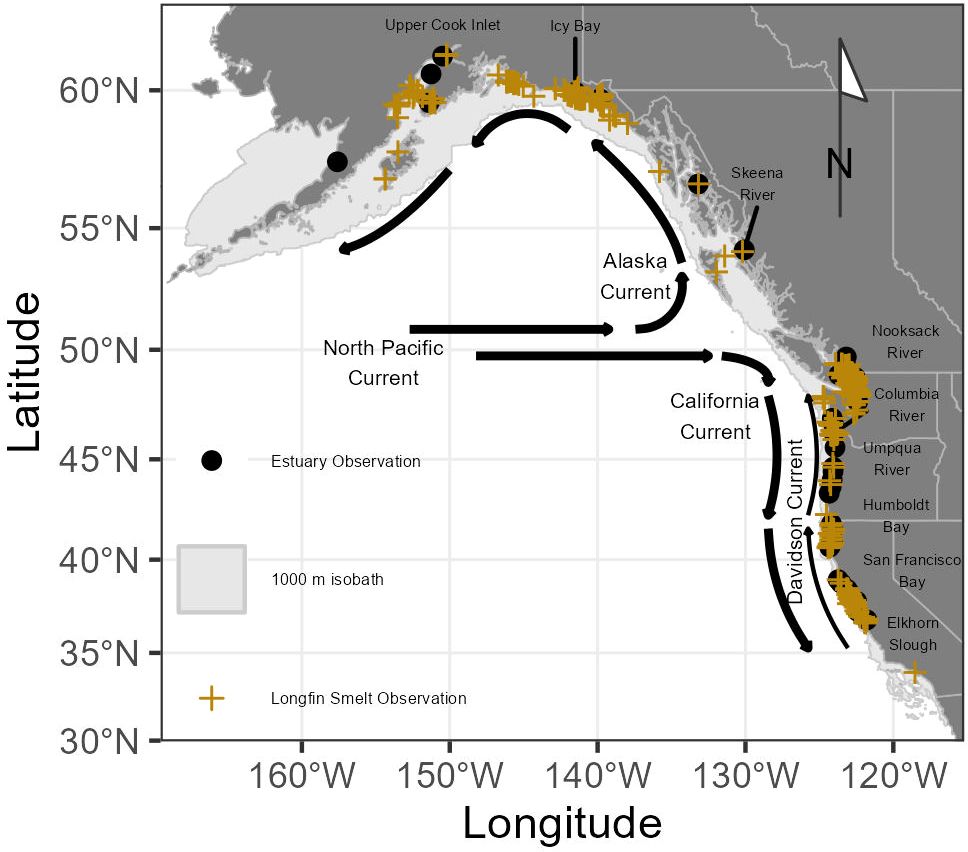
Figure 1 Map of the northeast Pacific Ocean displaying dominant ocean currents. Marine Longfin Smelt observations are shown with yellow crosses and estuaries with recorded Longfin Smelt observations within 1 km are noted with black circles and notable estuaries labeled. The 1000 m isobath is indicated by a light gray polygon.

Occurrence data for Longfin Smelt in marine habitats were compiled from a variety of regular and intermittent surveys (Figure 1; Young and Feyrer, 2022). These include oceanographic surveys conducted by National Oceanic and Atmospheric Administration (NOAA) Fisheries (https://www.fisheries.noaa.gov/) along the Pacific coast of North America, coastal observations by municipal, local, and state agencies (e.g., City of San Francisco, California Department of Fish and Wildlife), natural history museum collections, and other available records (e.g., Litz et al., 2014; Arimitsu et al., 2017; Garwood, 2017). When available, additional metadata (date, location, locality, counts) were included. In addition to compilation of all Longfin Smelt observations, we also compiled a list of estuaries where Longfin Smelt were captured within 1 km of the estuary mouth (Supplementary Table S1), suggesting the possibility that these estuaries may be spawning habitat. All data received a reliability rating, with reliability determined by consistency between site descriptions and available GPS coordinates, sample age, and spatial outliers (for further details see Young and Feyrer, 2022). Observations not deemed reliable were excluded from statistical analyses.

There were 882 unique, reliable coastal observations of Longfin Smelt, ranging from the Nushagak River estuary, Alaska, to coastal Santa Monica, California, and representing a period ranging from 1883 to 2019 (Table 1; Figure 1), with most observations (483) occurring between 1982 and 2012. Observations from the northwesternmost (Nushagak River, Bristol Bay, Alaska) and southernmost (San Pedro Channel near Santa Monica, California) locations were excluded from species distribution models because they were clear visual spatial outliers. Most coastal observations came from Washington (n = 408, ~46%), largely from Puget Sound and the San Juan Islands with coastal Alaska observations (n = 161, ~18%, largely near Cook Inlet and Icy Bay) next most frequent. Observations off the Oregon (n = 13) and British Columbia (n = 37) coasts were notably sparse, potentially due to lower sampling effort or inconsistent species identification on these coastlines. Thirty-seven estuaries had recorded Longfin Smelt presence (Figure 1; Supplementary Table S1). Sampling gear was noted for 688 observations. Of these, bottom trawls accounted for 437 observations (~64%), surface gears (surface trawls and purse seines) accounted for 228 observations (~33%), and shoreline-oriented gears (beach seines) accounted for 22 observations (3%). Due to inclement weather during winter and spring seasons there were few observations recorded north of Vancouver Island outside of the May through October period. Size data and life stage data were rarely available, so all observations were treated equally.

Table 1

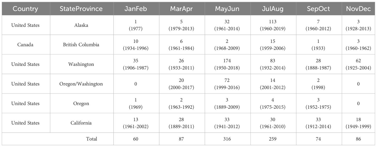
Table 1 Counts of Longfin Smelt observations summarized by region and bimonthly period, with observation data range included in parentheses.

2.2 Environmental data

Within the study region, we hypothesized that four continuous covariates were likely to influence Longfin Smelt distribution: depth (bathymetry), distance from nearest estuary, sea surface temperature, and sea surface chlorophyll concentration (Figure 2). Depth was included as a covariate because Longfin Smelt are presumed to be largely coastal, at least during part of their marine residence (Merz et al., 2013), and distance from nearest estuary was included because estuaries are known spawning habitats. Sea surface temperature and chlorophyll concentration (as a measure of ocean productivity) are both oceanographic parameters that commonly influence the distribution of forage fish (Cavole et al., 2016).

Figure 2

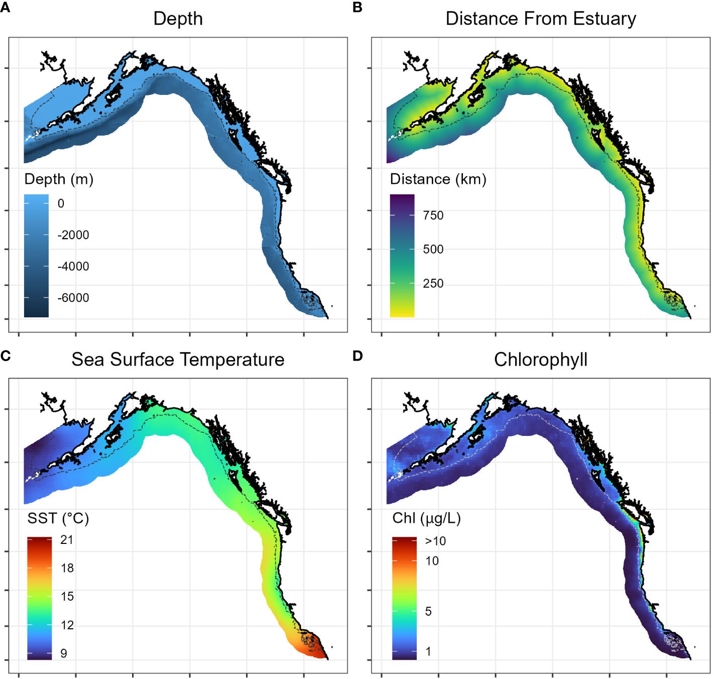
Figure 2 Representative maps of range-wide continuous covariates included in Longfin Smelt species distribution models, including (A) depth, (B) distance from estuary, (C) sea surface temperature (long-term mean 1981-2010), and (D) sea surface chlorophyll concentration (long-term mean 1981-2010). Gray dotted line denotes model domain boundary for species distribution model. See Methods for description of data sources.

We retrieved bathymetric depth data at the scale of at least 3 arc-seconds from NOAA’s bathymetry repository including the Pacific coast (NOAA National Geophysical Data Center, 2003a, 2003b, 2003c), southeast Alaska (NOAA National Geophysical Data Center, 2009), and British Columbia (Carignan et al., 2013). Retrieved bathymetry rasters were combined using commercial GIS software (ArcGIS Pro 2.5.0). To calculate distance from nearest estuary, we first extracted hydrographic data for the entire study region from the hydrographic dataset HydroRIVERS (Lehner and Grill, 2013) obtained from the repository HydroSHEDS (hydrosheds.org). Using HydroRIVERS, we extracted the mean annual discharge (1971-2000) from every estuary where Longfin Smelt were captured (Supplementary Table S1) and used the smallest of these discharges as a threshold (~ 10 m³ s^-1) to exclude smaller watersheds. We then calculated the covariate “Distance from Estuary” as the distance of each point in the sampling region to the nearest estuary that exceeded this discharge threshold as a continuous raster.

For range-wide distribution (Objective 1) and habitat suitability in the California Current ecosystem (Objective 2) oceanographic data were obtained from the World Ocean Atlas (Boyer et al., 2018, www.nodc.noaa.gov/OC5/woa13/). We extracted mean monthly ocean surface temperature (Locarnini et al., 2013) at the highest resolution grid available (0.25°) based on 1981-2010, a period encompassing most observations and for which data were already compiled. Satellite-derived mean monthly chlorophyll densities were obtained from NOAA’s COPEPOD project (National Oceanographic and Atmospheric Administration CoastWatch Program, 2022) toolkit at the same resolution and year range. For interannual analyses (Objective 3), we focused on the years 2002 through 2021, when high resolution sea surface chlorophyll data were available and to focus on how habitat suitability may have recently changed. Oceanographic data were obtained from NOAA’s ERDDAP server (National Oceanographic and Atmospheric Administration, 2022a) using the packages ‘rerrdap’ (Chamberlain et al., 2022) and ‘rerddapXtracto’ (Mendelssohn, 2021) in Program ‘R’ (R Core Team, 2022). Monthly composites of sea surface temperature (Saha et al., 2018) and sea surface chlorophyll concentration (National Oceanographic and Atmospheric Administration CoastWatch Program, 2022) were downloaded for the period between May 1 and June 30, and the period from July 1 and August 31, for every year from 2002 to 2021 at a 4 km grid and averaged to account for missing data. All pixels still missing data were interpolated using thin spline regression (function ‘Tsp’) from the package ‘fields’ (Nychka et al., 2022) in Program R. All physical and oceanographic covariates were overlaid on a 5 km spatial grid of the entire study region, spatially joined to the nearest grid point, and then converted to continuous raster files for subsequent statistical analysis.

2.3 Species distribution models

We used species distribution models to identify the range-wide distribution of Longfin Smelt and important environmental drivers of habitat suitability within the California Current ecosystem. Longfin Smelt occurrence data included primarily presence-only records, and thus we needed to use an analytical approach that was capable of drawing inference from presence-only data. By definition there is no verifiable absence in presence-only data, making it assess whether a lack of observation in a given area is due to real absence, a failure to detect, or no effort. Maximum entropy models have been developed as a prominent tool to address this type of data (Elith et al., 2011; Valavi et al., 2022). We developed Longfin Smelt distribution models using a maximum entropy approach (Phillips et al., 2006) with the package ‘MIAmaxent’ (Vollering et al., 2019) in program ‘R’ (R Core Team, 2022). Generally, maximum entropy models compare probability distribution in covariate space based on the conditional density of covariates at presence sites and the marginal density of covariates across the study area. These marginal densities are obtained from ‘pseudo-absences’ consisting of background points randomly chosen from the extent of the study region (see Figure 1). MIAmaxent uses subset selection to reduce the number of predictors to account for collinear covariates, reduce the need for prescreening variables, and develop ecologically interpretable models (Vollering et al., 2019).

We included physical and oceanographic environmental covariates to explain Longfin Smelt distribution and evaluate the relative contribution of each variable to model fit. To assess rangewide distributional drivers (Objective 1), we focused on the entire study region located between the northern and southernmost recorded observations (Figure 1), while for the California Current ecosystem (Objectives 2 and 3) we focused on the study region south of 50° N. For rangewide distribution (Objective 1), we developed Longfin Smelt distribution models for three bimonthly periods (May/June, July/August, and September/October), excluding months where data from the northern extent of the range were sparse or absent. For California Current distribution (Objective 2), we built Longfin Smelt distribution models within the California Current ecosystem for six bimonthly periods (January/February, March/April, May/June, July/August, September/October, November/December) using Longfin Smelt occurrence data south of 50° N. Bimonthly models were implemented to account for variation in environmental relationships that might be due to life history; for example, ‘Distance from Estuary’ may be more important during periods where Longfin Smelt are migrating toward or staging near spawning estuaries. For assessing interannual variability within the California Current ecosystem (Objective 3), we quantified Longfin Smelt habitat suitability in May/June and July/August for the years 2002-2021 by applying the species distribution model built in Objective 2 to year-specific oceanographic conditions. We evaluated May/June and July/August because these periods had the most observations within the California Current ecosystem. Habitat suitability results were presented for the entirety of the California Current and separately for the southern portion of their range (southward of Cape Blanco, Oregon, USA). Predicted habitat suitability was then compared to major oceanographic climate indices (i.e., PDO, NPGO, ENSO) using linear regression.

Maximum entropy analysis with MIAmaxent fits multiple derived variables (i.e., transformations, including linear, deviation, spline, and threshold transformations) of explanatory variables against occurrence data and pseudo-absences to allow for flexibility in quantifying non-linear relationships between species and habitat. Models were selected using forward stepwise selection using two steps (Halvorsen et al., 2015; Vollering et al., 2019). First, the best-fitting derived variable (i.e., transformation) for each explanatory variable (e.g., depth, temperature) is selected. Second, combinations of the best-fitting derived variables are compared to identify the best-fitting model.

Variable transformation was implemented using default MIAmaxent settings. Six transformation types were applied to continuous variables: linear, monotonous, deviation, forward hinge, reverse hinge, and threshold, with automatic transformation selection based on maximizing variation explained (Halvorsen et al., 2015). Models were selected based on the fraction of null deviance explained by each model during the selection process (Mazzoni et al., 2015).

Model performance was evaluated using the area under the curve (AUC) of the receiver operating characteristic. Model predictions were generated across the model domain in probability ratio output (PRO). PRO represents the “relative suitability of one place versus another” (Vollering et al., 2019). PRO has a range from 0 to ∞, with PRO = 1 representing the “average” suitability of the data. Values above 1 indicate higher-than-average probability of presence and values below 1 indicate lower-than-average probability of presence. Because “average” suitability may not be sufficient to quantify habitat, we categorized habitat suitability as weakly suitable (PRO between 0.5 and 1.5), moderately suitable (PRO between 1.5 and 5), and highly suitable (PRO > 5).

3 Results

3.1 Objective 1 – range-wide distribution of Longfin Smelt

Range-wide maximum entropy models constructed for all three bimonthly periods (May-June, July-August, September-October) identified suitable Longfin Smelt habitat within the study region. Average area under the curve (AUC) values based on the calibration data for the best-fitting models from all three bimonthly periods exceeded 0.9 (Table 2). As determined by model selection, ocean depth and sea surface temperature were important covariates in the best-fitting models for all bimonthly periods, distance from estuary was an important covariate in May-June and July-August, and sea surface chlorophyll was an important covariate in May-June and September-October (Figure 3, see Supplementary Table S2 for full model selection). Sea surface temperature had the highest fraction of total variation accounted (FTVA) in May-June (0.654), distance from estuary had the highest FTVA in July-August (0.717), and sea surface chlorophyll had the highest FTVA in September-October (0.760). The range of suitable Longfin Smelt habitat, as defined by PRO > 0.5 during any of the three modeled bimonthly periods, was contracted toward shore relative to the range described by the online repository FishBase (Froese and Pauly, 2023; Figure 4). In particular, the range of suitable habitat extended farther north and south than indicated by FishBase, and our models indicated that Longfin Smelt were closely tied to coastal shelf and nearshore waters. For model validation, range-wide models were repeated using only observations between 1982 and 2012, which directly correspond to the temporal period covered by oceanographic data. Predicted habitat suitability was similar (Supplementary Figure S1).

Table 2

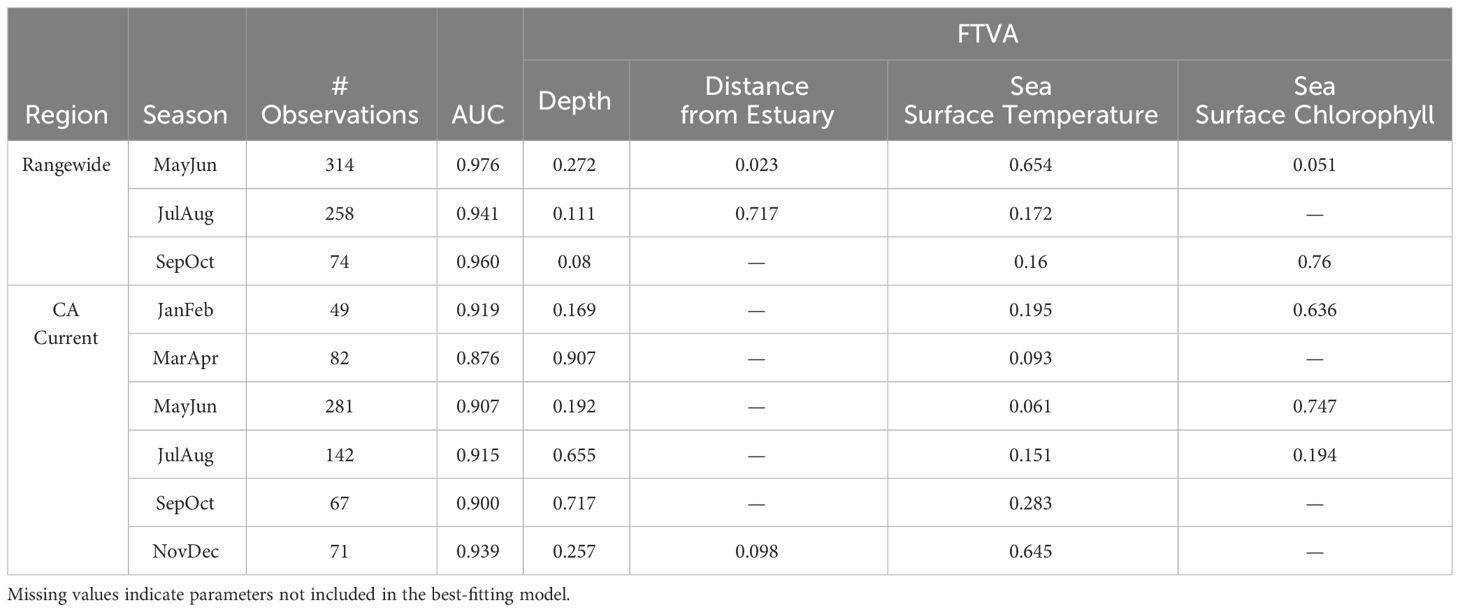
Table 2 Summary of best-fitting species distribution models by region and season. Includes area-under-the-curve (AUC) for each model, plus the fraction of the total variation accounted (FTVA) for each parameter included in the best-fitting model.

Figure 3

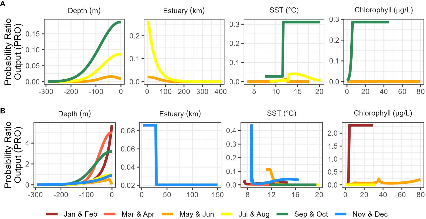
Figure 3 Marginal response curves for best-fitting range-wide (A) and California Current (B) species distribution models.

Figure 4

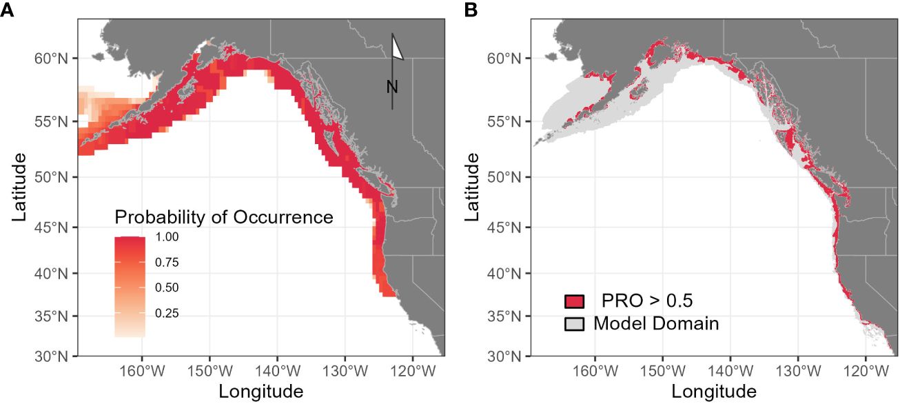
Figure 4 Range-wide distribution of Longfin Smelt as estimated by Fishbase (A; fishbase.org) and by species distribution models from this analysis (B), where potentially suitable habitat is defined as model probability ratio output greater than 0.5 from any of the three modeled seasons (May-June, July-August, September-October). Gray shading (B) indicates total model domain. Although direct comparisons with probability of occurrence are not possible, PRO = 1 is approximately equivalent to 50% probability of occurrence.

3.2 Objective 2 – California Current ecosystem habitat drivers

Maximum entropy models for the California Current ecosystem adequately identified suitable Longfin Smelt habitat in all bimonthly periods (AUC > 0.87; Table 2). As determined by model selection, ocean depth and sea surface temperature were important covariates in the best-fitting models for all bimonthly periods, distance from estuary was an important covariate in November-December, and sea surface chlorophyll was an important covariate in January-February, May-June, and July-August (Figure 3, see Supplementary Table S3 for full model selection). Sea surface chlorophyll was the most influential covariate in January-February (FTVA = 0.636) and May-June (FTVA = 0.747). Depth was the most influential covariate in March-April (FTVA = 0.907), July-August (FTVA = 0.655) and September-October (FTVA = 0.717), and sea surface temperature was the most influential covariate in November-December (0.645). Availability of suitable habitat (PRO > 0.5) across the California Current ecosystem (Table 3) was lowest in November-December (26.6% of modeled domain) and highest in September-October (39.0%). Habitat suitability at the southern extent of the range of Longfin Smelt (the coast of the State of California, south of 42° N) was lowest in March-April (19.1% of modeled domain) and highest in November-December (29.1%). This seasonal variability in predicted habitat suitability at the southernmost extent of the model domain was used to target model predictions for interannual variability in habitat suitability.

Table 3

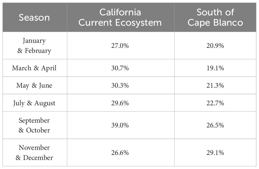
Table 3 Percent of modeled domain (see Figure 2) that is potentially suitable habitat for Longfin Smelt (Probability Ratio Output > 0.5) for each modeled season and sub-domain (the entire California Current ecosystem, and the coast south of Cape Blanco).

3.3 Objective 3 – habitat suitability over time

We predicted habitat suitability for Longfin Smelt for the years 2002-2021 for May/June and July/August, with habitat suitability varying across years (Figure 5). Average predicted suitable habitat in the entirety of the California Current ecosystem across all years was 35.8% of the modeled domain in May/June and 35.3% of the modeled domain in July/August, ranging between 10.5% (2005) and 35.8% (2007) in May/June, and ranging between 32.8% (2019) and 39.5% (2014) in July/August. Across the entire California Current ecosystem in May/June, there were frequent strong fluctuations (~10-20%), with more frequent positive values prior to 2010 and more frequent negative values after, except for 2014 which had a notable positive habitat expansion. For the entire California Current ecosystem in July/August, predicted suitable habitat was above average prior to 2009 and generally below average after, with a prominent exception in 2014 when the extent of predicted suitable habitat was the highest in the time series (an expansion of 9.9% suitable habitat relative to average). Despite observed variability in July/August, fluctuations never exceeded changes greater than 10% relative to average.

Figure 5

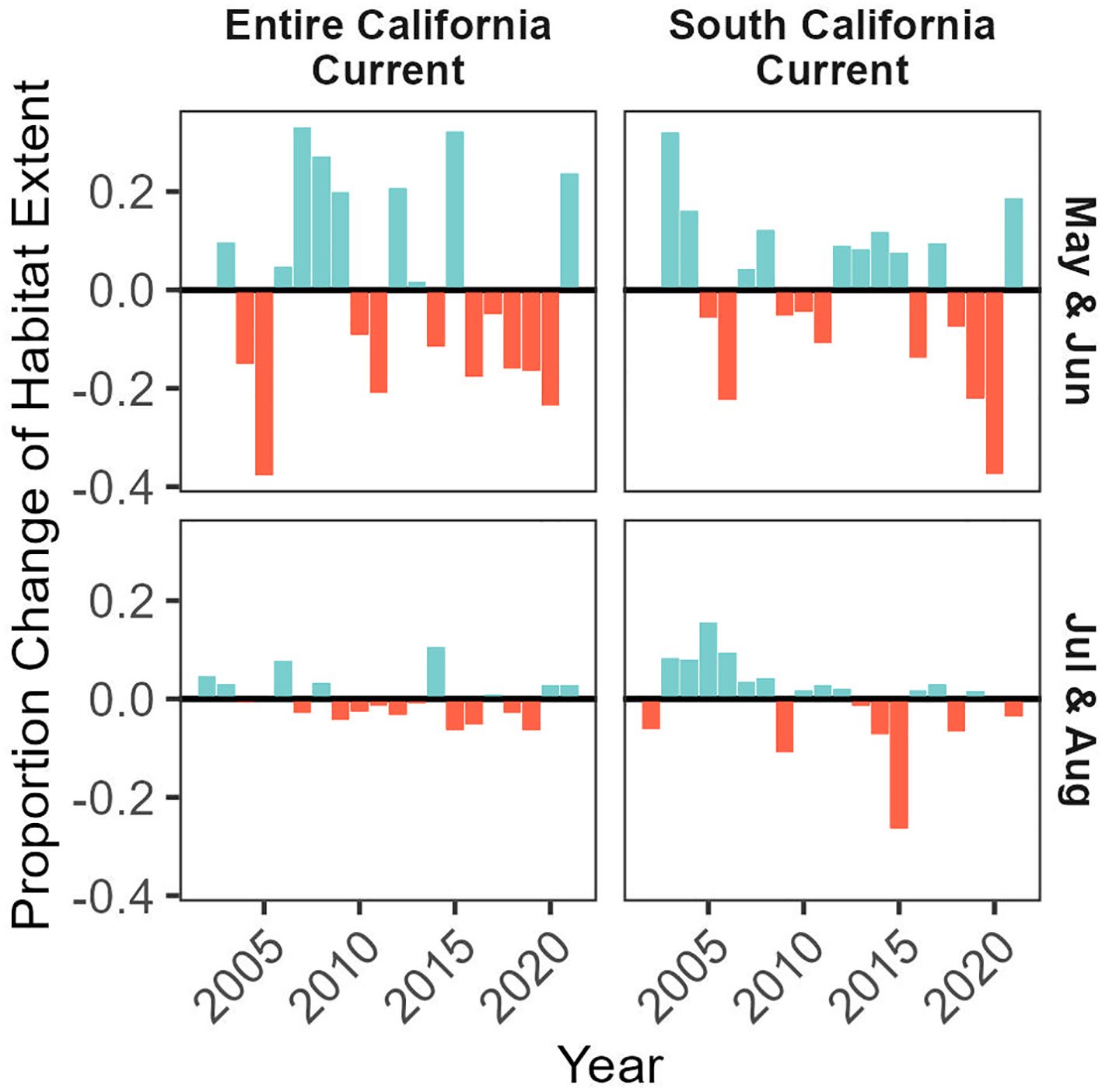
Figure 5 Proportion of potentially suitable habitat (probability ratio output > 0.5) within the modeled domain of the entire California Current ecosystem (top panel) and the southern California Current ecosystem including the California coastline (bottom panel). Values are expressed relative to mean habitat extent (from 2002-2021), and habitat expansions are colored blue and contractions are colored red.

In contrast, predicted suitable habitat along the California coast averaged 18.9% of the model domain in May/June, ranging between 8.5% (2020) and 27.8% (2003), and 25.6% of the model domain, ranging between 17.6% (2015) and 30.2% (2005). In May/June, the southern extent of the California Current (including the California coast), exhibited less variability than the entire California Current ecosystem, but habitat contractions were most consistent from 2015-2020 (Figure 6). Overall, predicted habitat suitability was lower along the California coast than the entirety of the California Current ecosystem, and exhibited similar (May/June) or higher (July/August) variability in the extent of suitable habitat.

Figure 6

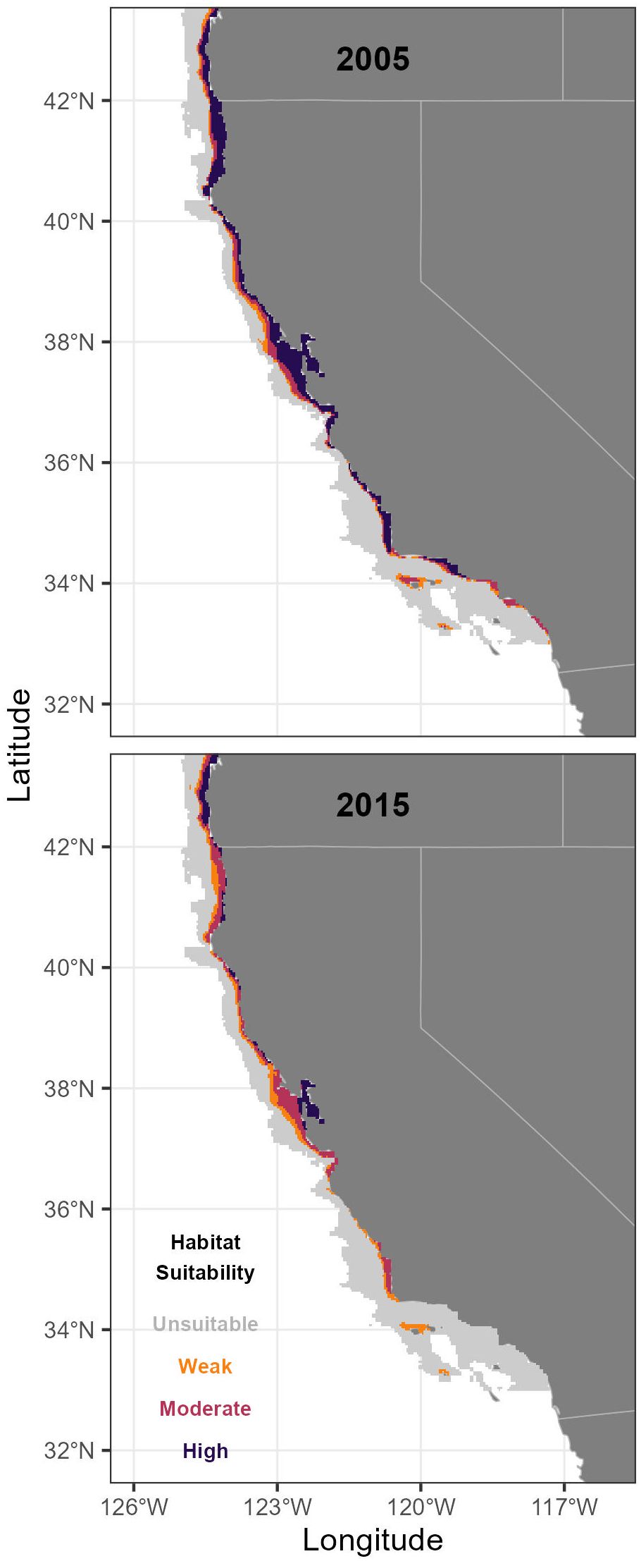
Figure 6 Longfin Smelt habitat suitability along the southern California Current ecosystem including the California coast for the highest (2005) and lowest (2015) habitat suitability years (see Figure 3). Unsuitable habitat had a modeled probability ratio output (PRO) of <0.5, weakly suitable had a PRO between 0.5 and 1.5, moderately suitable had a PRO between 1.5 and 5, and highly suitable had a PRO > 5.

After correcting for multiple tests there were no statistically significant relationships between climate indices and predicted habitat suitability (Supplementary Figure S2), although there was evidence that PDO and NPGO may have some influence on habitat suitability. Generally, variability in climate indices had stronger associations with habitat suitability in May and June, with no associations between climate indices and habitat suitability in July and August. A positive NPGO index associated with improved habitat suitability across both the entire California Current ecosystem and the southern extent (California coast). Positive ENSO and PDO values were negatively associated with habitat suitability across the entire California Current, but associations were weaker in the southern extent.

4 Discussion

Understanding the environmental conditions and processes that affect species of management concern can be especially difficult for species that encompass broad latitudinal and environmental gradients such as Longfin Smelt. We used sparse observational data to identify coarse habitat drivers across the entire range of Longfin Smelt, gain insight into how habitat suitability has changed over time, and enhance existing knowledge of Longfin Smelt habitat in the northeast Pacific Ocean. Many fish species that are not the subject of targeted monitoring efforts are similarly data limited, and this approach could provide a model for other fish species with limited data.

4.1 Longfin Smelt marine habitat

Longfin Smelt were predominately associated with coastal, shallow habitat throughout the entirety of its range. These habitat associations are generally consistent with those of other osmerid species in the northeast Pacific Ocean, particularly the anadromous Eulachon (Allen and Smith, 1988; Montgomery, 2020). Notably, in regions and surveys where data from benthic and surface trawls were available (e.g., Puget Sound; coastal habitats within the California Current ecosystem), Longfin Smelt observations from benthic trawls were more prevalent. This indicates the potential for Longfin Smelt to spend more time closer to the ocean bottom than the surface, similar to Eulachon (Hay and McCarter, 2000). Collectively, this presents Longfin Smelt as a species tightly tied to shallow coastal waters, with potential habitat ranging from the Southern California Bight, California, in the south to Bristol Bay, Alaska, in the north, with the core, higher probability habitat ranging from Monterey Bay, California, in the south to Cook Inlet, Alaska, in the north.

There was evidence for use of estuaries of varying size and structure, including large, river-dominated estuaries (e.g., San Francisco Estuary, Columbia River Estuary, Fraser River Estuary, Skeena River Estuary), embayments (e.g., Humboldt Bay, California; upper Cook Inlet, Alaska), lagoons (e.g., Lake Earl and Russian River, California), and the network of fjords, bays, and river mouths comprising Puget Sound, Washington. We found evidence for Longfin Smelt use of large glacial fjords (e.g., Kachemak Bay, Icy Bay, Yakutat Bay; Alaska), but the extent to which Longfin Smelt are broadly associated with fjord-like systems is unknown. Few Longfin Smelt were observed in the Alexander Archipelago, an approximately 480-km long archipelago in southeast Alaska, which is dominated by narrow fjords with steep coastlines and deep channels, or from the coast between the Skeena and Fraser Rivers, which is similarly fjord-dominated. This lack of observations may result from bias in data availability or may indicate that these habitats are suboptimal for Longfin Smelt. Notably, Eulachon are frequently encountered in offshore research surveys and are known to spawn in many rivers feeding these fjords (Hay and McCarter, 2000; Sutherland et al., 2021), but Longfin Smelt have not been reported.

In many instances, routine coastal fish community surveys and commercial bycatch monitoring do not consistently distinguish Longfin Smelt from similar species in the family Osmeridae (e.g., Night Smelt Spirinchus starksi, Whitebait Smelt Allosmerus elongatus, Surf Smelt Hypomesus pretiosus). This lack of distinction among species limits our understanding of the distribution of osmerid fishes in the northeast Pacific Ocean because verifiable absences cannot be distinguished; therefore, our dataset is compiled of documented positive observations only. The consistent identification of Eulachon by fish surveys and bycatch monitoring has provided substantial information on the distribution of that species across a wide array of habitats and locations (Wargo et al., 2014), which may indicate that Longfin Smelt occupy more habitats than recognized by this dataset.

Although the presence-only dataset in this study has limitations, maximum entropy models used here provide substantial insights into the nuances of Longfin Smelt distribution in the Pacific Ocean. In particular, this analysis identified potential suitable habitat closer to shore, and the suitable habitat extends farther north and south than was indicated by FishBase (Froese and Pauly, 2023). Refined estimates of suitable habitat have implications for conservation of appropriate habitat at the southern extent of its range and the potential for northward expansion of Longfin Smelt habitat as oceanic conditions change (Canning-Clode and Carlton, 2017). These results indicate the importance of using intentionally chosen modeling approaches to assess fish distribution, particularly for data-limited species with broad distributions.

4.2 The California Current ecosystem

The California Current ecosystem is highly productive, heterogeneous, and relatively consistent habitat for Longfin Smelt. Throughout both the Alaska and California currents, most Longfin Smelt observations occurred in regions with ocean depths less than 200 m, and few Longfin Smelt were observed in areas with ocean depths greater than 400 m. However, the California Current ecosystem is a narrow continental shelf of the coastline. This means that the spatial footprint of suitable habitat is relatively narrow in the California Current, especially south of Cape Blanco, Oregon.

Within the California Current ecosystem, sea surface temperature consistently affected Longfin Smelt distribution across all seasons. The California Current ecosystem encompasses the California coast, which is the southern extent of Longfin Smelt range. The importance of sea surface temperature to Longfin Smelt is consistent with many organisms observed at the edge of their range. Fluctuations in important clinal habitat elements that vary with latitude can exceed physiological preferences and/or tolerances and can drive poleward migrations (Murawski, 1993) or equatorial habitat contractions as oceans warm nearer the equator. These relationships can be complicated because not every equator-ward contraction is offset by poleward expansions. Although little is known about ideal temperature ranges in the ocean, in fresh waters of the San Francisco Estuary, post-larval and juvenile Longfin Smelt are generally found in temperatures less than 18°C (Moyle, 2002; Jeffries et al., 2016). This temperature threshold can be approached or exceeded in coastal marine habitats south of Point Conception (Santa Barbara County, California) and at points north during warm years (like those often observed when the El Niño Southern Oscillation index is positive) or when coastal upwelling is otherwise curtailed (Locarnini et al., 2013).

Relationships between oceanographic indices and habitat suitability were not statistically significant based on linear regression coefficients, but this lack of statistical significance does not mean that oceanographic indices do not influence predicted habitat suitability. Oceanographic conditions along the California coast have been highly variable over the past several decades, with commensurate variability in the distribution of forage fish and crustaceans in the California Current (Muhling et al., 2020; Phillips et al., 2022). The ENSO index is an important driver of California coastal conditions and has varied from the highest on record in 2015-2016 (El Niño conditions, typically warmer than average) to very low in 2007-2008 and 2010-2011 (La Niña conditions, typically cooler than average). The PDO, which historically would fluctuate from “warm” to “cool” phases on decadal time scales, has exhibited higher-frequency variability since 1999 (National Oceanographic and Atmospheric Administration, 2022b), as has the NPGO (Di Lorenzo, 2008). Generally, variability in climate indices had a stronger impact on habitat suitability in May and June, suggesting that conditions in the ocean immediately upon migration from estuarine habitats may be a key factor driving Longfin Smelt recruitment success, consistent with both Eulachon (Montgomery, 2020) and Chinook Salmon (Duffy and Beauchamp, 2011; Tomaro et al., 2012).

In addition to these modes of oceanographic variability, an anomalously warm water “Blob” heavily influenced the northeastern Pacific Ocean, including the California Current ecosystem, from 2013-2015. This persistent and extreme marine heatwave was at times characterized by ENSO-, NPGO-, and PDO-like variability (Di Lorenzo and Mantua, 2016), and was associated with dramatic shifts in distribution and abundance of many taxa (Cavole et al., 2016), including forage fish such as Pacific Sardine Sardinops sagax and Northern Anchovy Engraulis mordax (Muhling et al., 2020).

It is likely that the Blob and the strong El Niño of 2015-2016, which represented the warmest 3-year period dating back to at least 1920 (Jacox et al., 2018), had significant negative impacts on Eulachon (Gustafson et al., 2012) and corresponds to the lowest extent of habitat suitability for Longfin Smelt along the California coast in July and August. Possible mechanisms for this reduction in habitat could include direct temperature effects, whereby temperatures would exceed preferences or tolerances, or they could be indirect effects, whereby temperature mediates other oceanographic factors. For example, coastal productivity in this region is heavily influenced by upwelling strength (Black et al., 2011; Jacox et al., 2014), and changes in prey availability or composition tied to coastal upwelling may be associated with Longfin Smelt habitat suitability.

4.3 The black box of Longfin Smelt life history

Forage fish productivity in coastal ecosystems is heavily influenced by interactions between zooplankton production and piscivore predation on forage fishes and, for species which require low-salinity environments, variation in freshwater flow rates. Extensive exploration of the Longfin Smelt life cycle has documented the importance of freshwater outflow to Longfin Smelt production in the San Francisco Estuary (Jassby et al., 1995; Kimmerer, 2002; Rosenfield and Baxter, 2007; Nobriga and Rosenfield, 2016) and Lake Washington (Chigbu, 2000). Ocean conditions have had demonstrable impacts on Longfin Smelt recruitment (Feyrer et al., 2015), but mechanisms are poorly understood. There is strong density dependence and declining survival during the transition from age 0 fish in the San Francisco Estuary to age 2 fish that have returned to the San Francisco Estuary (Nobriga and Rosenfield, 2016), and these density-dependent relationships can be caused by food-web-related mechanisms (Walters and Juanes, 1993). Because San Francisco Estuary Longfin Smelt are in the ocean between ages 0 and 2, the mechanisms that are causing density-dependent survival and declines in overall survival are likely tied to ocean conditions and possible bottom-up effects; however, additional data would be needed to confirm this hypothesis. This could include many possible mechanisms, as changing environmental conditions can affect prey availability for Longfin Smelt, but also the potential for prey-switching by possible predators, as seen for Chinook Salmon Oncorhychus tshawytscha (Wells et al., 2017).

There is strong evidence for variability in Longfin Smelt habitat suitability associated with fluctuating environmental conditions, but recent oceanographic conditions have been outside of the range of historical measurements. These extreme events have led to notable reductions in predictive capacity for Pacific Sardine and Northern Anchovy species distribution models trained on historical data (Muhling et al., 2020). Our models likely have similar limitations that are further exacerbated by the lack of Longfin Smelt data relative to Pacific Sardines or Northern Anchovy. Despite this constraint, these analyses indicate substantive variability in Longfin Smelt ocean habitat, with additional work needed to clearly identify mechanisms and contextualize further environmental change. Most importantly, additional data collection would increase opportunities for inference.

Presence-only methods (such as maximum entropy analysis) are unable to definitively address occupancy or population characteristics (such as abundance). Consistent identification of Longfin Smelt by ongoing marine fisheries surveys would provide recent and reliable presence-absence and count data, improving species distribution models and allowing for a wider array of statistical techniques that could be used to address additional facets of Longfin Smelt distributional drivers in the Pacific Ocean. While Longfin Smelt presumably forage largely on zooplankton and euphausiids while in the ocean, a comprehensive assessment of diet, condition, and distribution of subadult Longfin Smelt would help identify mechanisms by which oceanographic conditions and bottom-up influences control marine drivers of Longfin Smelt population dynamics. The Longfin Smelt life cycle is complex, and comprehensive assessment of all phases could help inform appropriate management of the species.

Data availability statement

The datasets presented in this study can be found in online repositories. The names of the repository/repositories and accession number(s) can be found below: https://doi.org/10.5066/P9Z9FASJ.

Ethics statement

Ethical approval was not required for the study involving animals in accordance with the local legislation and institutional requirements because this study compiled already existing observations of a vertebrate in the wild, and did not require physical capture or handling of organisms.

Author contributions

MY: Writing – review & editing, Writing – original draft, Project administration, Methodology, Investigation, Formal analysis, Data curation, Conceptualization. FF: Writing – review & editing, Supervision, Project administration, Investigation, Funding acquisition, Data curation, Conceptualization. SL: Writing – review & editing, Conceptualization. DH: Writing – review & editing.

Funding

The author(s) declare financial support was received for the research, authorship, and/or publication of this article. Funding was provided by the State Water Contractors.

Acknowledgments

Numerous individuals exchanged correspondence to help interpret data included in the underlying distribution dataset, including J. Blaine, A. Chang, A. Chappell, J. Cleary, C. Flannery, L. Flostrand, L. Granum, C. Greene, J. Harding, T. McKinley, C. Morgan, D. Neff, J. Phillips, K. Somers, W. Wakefield, and L. Weitkamp. The authors would like to thank three reviewers and Caitlin Marsteller for providing feedback that greatly improved this manuscript. Any use of trade, firm, or product names is for descriptive purposes only and does not imply endorsement by the U.S. Government.

Conflict of interest

The authors declare that the research was conducted in the absence of any commercial or financial relationships that could be construed as a potential conflict of interest.

The reviewer CG declared a shared affiliation with the author DH to the handling editor at the time of review.

Publisher’s note

All claims expressed in this article are solely those of the authors and do not necessarily represent those of their affiliated organizations, or those of the publisher, the editors and the reviewers. Any product that may be evaluated in this article, or claim that may be made by its manufacturer, is not guaranteed or endorsed by the publisher.

Supplementary material

The Supplementary Material for this article can be found online at: https://www.frontiersin.org/articles/10.3389/fmars.2024.1282286/full#supplementary-material

References

Allen M. J., Smith G. B. (1988) Atlas and zoogeography of common fishes in the Bering Sea and northeastern Pacific. Available online at: https://repository.library.noaa.gov/view/noaa/5807/noaa_5807_DS1.pdf. doi: 10.5962/bhl.title.62517

CrossRef Full Text | Google Scholar

Arimitsu M. L., Piatt J. F., Heflin B. (2017). Influence of Glacier Run Off on Ecosystem Structure in Gulf of Alaska Fjords 2004-2011: U.S. Geological Survey data release. Anchorage, Alaska, USA: U.S. Geological Survey. doi: 10.5066/F7K072DR

CrossRef Full Text | Google Scholar

Black B. A., Schroeder I. D., Sydeman W. J., Bograd S. J., Wells B. K., Schwing F. B. (2011). Winter and summer upwelling modes and their biological importance in the California Current Ecosystem. Glob. Change Biol. 17, 2536–2545. doi: 10.1111/j.1365-2486.2011.02422.x

CrossRef Full Text | Google Scholar

Bottom D. L., Jones K. K., Herring M. J. (1984). Fishes of the Columbia River estuary. Or. Dep. Fish Wildl. Columbia River Estuary Data Dev. Program Corvallis Or. 113. Available at: https://www.estuarypartnership.org/sites/default/files/resource_files/12%20-%20FISHES%20OF%20THE%20COLUMBIA%20RIVER%20ESTUARY.pdf.

Google Scholar

Boyer T. P., Garcia H. E., Locarnini R. A., Zweng M. M., Mishonov A. V., Reagan J. R., et al. (2018). World Ocean Atlas 2018. Available online at: https://www.ncei.noaa.gov/archive/accession/NCEI-WOA18 (Accessed June 1, 2022).

Google Scholar

Brennan C. A., Hassrick J. L., Kalmbach A., Cox D. M., Sabal M. C., Zeno R. L., et al. (2022). Estuarine recruitment of longfin smelt (Spirinchus thaleichthys) north of the San Francisco estuary. San Franc. Estuary Watershed Sci. 20. doi: 10.15447/sfews.2022v20iss3art3

CrossRef Full Text | Google Scholar

California Fish and Game Commission. (2009). Notice of findings: longfin smelt (Spirinchus thaleichthys). Available online at: https://web2.co.merced.ca.us/boardagenda/2009/MG145708/AS145762/AI146032/DO146079/all_pages.pdf (Accessed February 11, 2024).

Google Scholar

Canning-Clode J., Carlton J. T. (2017). Refining and expanding global climate change scenarios in the sea: Poleward creep complexities, range termini, and setbacks and surges. Divers. Distrib. 23, 463–473. doi: 10.1111/ddi.12551

CrossRef Full Text | Google Scholar

Carignan K. S., Eakins B. W., Love M. R., Sutherland M. G., McLean S. J. (2013) Bathymetric Digital Elevation Model of British Columbia, Canada: Procedures, Data Sources, and Analysis. Prepared for NOAA, Pacific Marine Environmental Laboratory (PMEL) by the NOAA National Geophysical Data Center (NGDC). Available online at: https://www.ngdc.noaa.gov/mgg/dat/dems/regional_tr/british_columbia_3_msl_2013.pdf.

Google Scholar

Cavole L. M., Demko A. M., Diner R. E., Giddings A., Koester I., Pagniello C. M., et al. (2016). Biological impacts of the 2013–2015 warm-water anomaly in the Northeast Pacific: winners, losers, and the future. Oceanography 29, 273–285. doi: 10.5670/oceanog

CrossRef Full Text | Google Scholar

Chamberlain S., Tupper B., Mendelssohn R. (2022). rerddap: General Purpose Client for “ERDDAP” Servers. Available online at: https://github.com/ropensci/rerddap (Accessed April 15, 2022).

Google Scholar

Chigbu P. (2000). Population biology of longfin smelt and aspects of the ecology of other major planktivorous fishes in Lake Washington. J. Freshw. Ecol. 15, 543–557. doi: 10.1080/02705060.2000.9663777

CrossRef Full Text | Google Scholar

Cloern J. E., Jassby A. D. (2012). Drivers of change in estuarine-coastal ecosystems: Discoveries from four decades of study in San Francisco Bay. Rev. Geophys. 50. doi: 10.1029/2012RG000397

CrossRef Full Text | Google Scholar

Cloern J. E., Jassby A. D., Thompson J. K., Hieb K. A. (2007). A cold phase of the East Pacific triggers new phytoplankton blooms in San Francisco Bay. Proc. Natl. Acad. Sci. 104, 18561–18565. doi: 10.1073/pnas.0706151104

CrossRef Full Text | Google Scholar

Di Lorenzo E. (2008) North Pacific Gyre Oscillation. Available online at: http://www.o3d.org/npgo/index.html (Accessed August 1, 2022).

Google Scholar

Di Lorenzo E., Mantua N. (2016). Multi-year persistence of the 2014/15 North Pacific marine heatwave. Nat. Clim. Change 6, 1042–1047. doi: 10.1038/nclimate3082

CrossRef Full Text | Google Scholar

Di Lorenzo E., Schneider N., Cobb K. M., Franks P., Chhak K., Miller A. J., et al. (2008). North Pacific Gyre Oscillation links ocean climate and ecosystem change. Geophys. Res. Lett. 35. doi: 10.1029/2007GL032838

PubMed Abstract | CrossRef Full Text | Google Scholar

Duffy E. J., Beauchamp D. A. (2011). Rapid growth in the early marine period improves the marine survival of Chinook salmon (Oncorhynchus tshawytscha) in Puget Sound, Washington. Can. J. Fish. Aquat. Sci. 68, 232–240. doi: 10.1139/F10-144

CrossRef Full Text | Google Scholar

Elith J., Phillips S. J., Hastie T., Dudík M., Chee Y. E., Yates C. J. (2011). A statistical explanation of MaxEnt for ecologists. Divers. Distrib. 17, 43–57. doi: 10.1111/ddi.2010.17.issue-1

CrossRef Full Text | Google Scholar

Feyrer F., Cloern J. E., Brown L. R., Fish M. A., Hieb K. A., Baxter R. D. (2015). Estuarine fish communities respond to climate variability over both river and ocean basins. Glob. Change Biol. 21, 3608–3619. doi: 10.1111/gcb.12969

CrossRef Full Text | Google Scholar

Froese R., Pauly D. (2023). FishBase. Available online at: www.fishbase.org.

Google Scholar

Garwood R. S. (2017). Historic and contemporary distribution of Longfin Smelt (Spirinchus thaleichthys) along the California coast. Calif. Fish Game 103, 96–117. Available at: https://nrm.dfg.ca.gov/FileHandler.ashx?DocumentID=152480.

Google Scholar

Gustafson R. G., Ford M. J., Adams P. B., Drake J. S., Emmett R. L., Fresh K. L., et al. (2012). Conservation status of eulachon in the California Current. Fish Fish. 13, 121–138. doi: 10.1111/j.1467-2979.2011.00418.x

CrossRef Full Text | Google Scholar

Halvorsen R., Mazzoni S., Bryn A., Bakkestuen V. (2015). Opportunities for improved distribution modelling practice via a strict maximum likelihood interpretation of MaxEnt. Ecography 38, 172–183. doi: 10.1111/ecog.00565

CrossRef Full Text | Google Scholar

Hay D., McCarter P. (2000). Status of the eulachon Thaleichthys pacificus in Canada (Nanaimo, B.C., CA: Canadian Stock Assessment Secretariat, Fisheries and Oceans Canada).

Google Scholar

Hickey B. M., Royer T. C. (2009). “California and Alaska currents,” in Ocean Currents Encycolopedia of Ocean Sciences (Oxford, UK: Elsevier).

Google Scholar

Hobbs J., Moyle P. B., Fangue N., Connon R. E. (2017). Is extinction inevitable for Delta Smelt and Longfin Smelt? An opinion and recommendations for recovery. San Franc. Estuary Watershed Sci. 15. doi: 10.15447/sfews.2017v15iss2art2

CrossRef Full Text | Google Scholar

Huyer A. (1983). Coastal upwelling in the California Current system. Prog. Oceanogr. 12, 259–284. doi: 10.1016/0079-6611(83)90010-1

CrossRef Full Text | Google Scholar

Jacox M. G., Alexander M. A., Mantua N. J., Scott J. D., Hervieux G., Webb R. S., et al. (2018). Forcing of multi-year extreme ocean temperatures that impacted California Current living marine resources in 2016. Bull. Amer. Meteor Soc. 99, S27–S33. doi: 10.1175/BAMS-D-17-0119.1

CrossRef Full Text | Google Scholar

Jacox M., Moore A., Edwards C., Fiechter J. (2014). Spatially resolved upwelling in the California Current System and its connections to climate variability. Geophys. Res. Lett. 41, 3189–3196. doi: 10.1002/2014GL059589

CrossRef Full Text | Google Scholar

Jassby A. D., Kimmerer W. J., Monismith S. G., Armor C., Cloern J. E., Powell T. M., et al. (1995). Isohaline position as a habitat indicator for estuarine populations. Ecol. Appl. 5, 272–289. doi: 10.2307/1942069

CrossRef Full Text | Google Scholar

Jeffries K. M., Connon R. E., Davis B. E., Komoroske L. M., Britton M. T., Sommer T., et al. (2016). Effects of high temperatures on threatened estuarine fishes during periods of extreme drought. J. Exp. Biol. 219, 1705–1716. doi: 10.1242/jeb.134528

PubMed Abstract | CrossRef Full Text | Google Scholar

Kimmerer W. (2002). Effects of freshwater flow on abundance of estuarine organisms: physical effects or trophic linkages? Mar. Ecol. Prog. Ser. 243, 39–55. doi: 10.3354/meps243039

CrossRef Full Text | Google Scholar

Latour R. J. (2016). Explaining patterns of pelagic fish abundance in the Sacramento-San Joaquin Delta. Estuaries Coasts 39, 233–247. doi: 10.1007/s12237-015-9968-9

CrossRef Full Text | Google Scholar

Lehner B., Grill G. (2013). Global river hydrography and network routing: baseline data and new approaches to study the world’s large river systems. Hydrol. Process. 27, 2171–2186. doi: 10.1002/hyp.9740

CrossRef Full Text | Google Scholar

Litz M. N., Emmett R. L., Bentley P. J., Claiborne A. M., Barceló C. (2014). Biotic and abiotic factors influencing forage fish and pelagic nekton community in the Columbia River plume (USA) throughout the upwelling season 1999–2009. ICES J. Mar. Sci. 71, 5–18. doi: 10.1093/icesjms/fst082

CrossRef Full Text | Google Scholar

Locarnini M., Mishonov A., Baranova O., Boyer T., Zweng M., Garcia H., et al. (2013). World Ocean Atlas 2018, Volume 1: Temperature. Available online at: https://www.ncei.noaa.gov/data/oceans/woa/WOA13/DOC/woa13_vol1.pdf.

Google Scholar

Lund J. R. (2016). California’s agricultural and urban water supply reliability and the Sacramento–San Joaquin Delta. San Franc. Estuary Watershed Sci. 14. doi: 10.15447/sfews.2016v14iss3art6

CrossRef Full Text | Google Scholar

Mac Nally R., Thomson J. R., Kimmerer W. J., Feyrer F., Newman K. B., Sih A., et al. (2010). Analysis of pelagic species decline in the upper San Francisco Estuary using multivariate autoregressive modeling (MAR). Ecol. Appl. 20, 1417–1430. doi: 10.1890/09-1724.1

PubMed Abstract | CrossRef Full Text | Google Scholar

Mantua N. J., Hare S. R., Zhang Y., Wallace J. M., Francis R. C. (1997). A Pacific interdecadal climate oscillation with impacts on salmon production. Bull. Am. Meteorol. Soc 78, 1069–1080. doi: 10.1175/1520-0477(1997)078<1069:APICOW>2.0.CO;2

CrossRef Full Text | Google Scholar

Maunder M. N., Deriso R. B., Hanson C. H. (2015). Use of state-space population dynamics models in hypothesis testing: advantages over simple log-linear regressions for modeling survival, illustrated with application to longfin smelt (Spirinchus thaleichthys). Fish. Res. 164, 102–111. doi: 10.1016/j.fishres.2014.10.017

CrossRef Full Text | Google Scholar

Mazzoni S., Halvorsen R., Bakkestuen V. (2015). MIAT: Modular R-wrappers for flexible implementation of MaxEnt distribution modelling. Ecol. Inform. 30, 215–221. doi: 10.1016/j.ecoinf.2015.07.001

CrossRef Full Text | Google Scholar

Mendelssohn R. (2021) rerddapXtracto: Extracts Environmental Data from “ERDDAP” Web Services. Available online at: https://github.com/rmendels/rerddapXtracto (Accessed April 15, 2022).

Google Scholar

Merz J. E., Bergman P. S., Melgo J. F., Hamilton S. (2013). Longfin smelt: spatial dynamics and ontogeny in the San Francisco Estuary, California. Calif. Fish Game 99, 122–148. Available at: https://nrm.dfg.ca.gov/FileHandler.ashx?DocumentID=75568.

Google Scholar

Montgomery S. A. (2020). Eulachon (Thaleichthys pacificus) marine ecology: applying ocean ecosystem indicators from salmon to develop a multi-year model of freshwater abundance (Seattle, WA: University of Washington). Available at: https://digital.lib.washington.edu/researchworks/bitstream/handle/1773/46088/Montgomery_washington_0250O_21907.pdf?sequence=1.

Google Scholar

Moyle P. B. (2002). Inland fishes of California: revised and expanded (Berkeley, CA: University of California Press).

Google Scholar

Muhling B. A., Brodie S., Smith J. A., Tommasi D., Gaitan C. F., Hazen E. L., et al. (2020). Predictability of species distributions deteriorates under novel environmental conditions in the California Current System. Front. Mar. Sci. 7. doi: 10.3389/fmars.2020.00589

CrossRef Full Text | Google Scholar

Murawski S. (1993). Climate change and marine fish distributions: forecasting from historical analogy. Trans. Am. Fish. Soc 122, 647–658. doi: 10.1577/1548-8659(1993)122<0647:CCAMFD>2.3.CO;2

CrossRef Full Text | Google Scholar

National Oceanographic and Atmospheric Administration (2022a) ERDDAP. Available online at: https://coastwatch.pfeg.noaa.gov/erddap/index.html (Accessed August 1, 2022a).

Google Scholar

National Oceanographic and Atmospheric Administration (2022b) Pacific Decadal Oscillation. Available online at: https://www.ncei.noaa.gov/access/monitoring/pdo/ (Accessed August 1, 2022b).

Google Scholar

National Oceanographic and Atmospheric Administration CoastWatch Program (2022) High Resolution Chlorophyll-a concentration from MODIS/Aqua. Available online at: https://coastwatch.pfeg.noaa.gov/infog/MW_chla_las.html (Accessed August 1, 2022).

Google Scholar

NOAA National Geophysical Data Center (2003a). U.S. Coastal Relief Model Vol.6 - Southern California. doi: 10.7289/V500001J

CrossRef Full Text | Google Scholar

NOAA National Geophysical Data Center (2003b). U.S. Coastal Relief Model Vol.7 - Central Pacific. doi: 10.7289/V50Z7152

CrossRef Full Text | Google Scholar

NOAA National Geophysical Data Center (2003c). U.S. Coastal Relief Model Vol.8 - Northwest Pacific. doi: 10.7289/V5H12ZXJ

CrossRef Full Text | Google Scholar

NOAA National Geophysical Data Center (2009). Southern Alaska Coastal Relief Model. (NOAA National Centers for Environmental Education). doi: 10.7289/V58G8HMQ

CrossRef Full Text | Google Scholar

Nobriga M. L., Rosenfield J. A. (2016). Population dynamics of an estuarine forage fish: disaggregating forces driving long-term decline of Longfin Smelt in California’s San Francisco Estuary. Trans. Am. Fish. Soc 145, 44–58. doi: 10.1080/00028487.2015.1100136

CrossRef Full Text | Google Scholar

Nychka D., Furrer R., Paige J., Sain S., Gerber F., Iverson M. (2022) fields: Tools for Spatial Data. Available online at: https://github.com/ropensci/rerddap (Accessed August 15, 2022).

Google Scholar

Peterson W. T., Fisher J. L., Strub P. T., Du X., Risien C., Peterson J., et al. (2017). The pelagic ecosystem in the Northern California Current off Oregon during the 2014–2016 warm anomalies within the context of the past 20 years. J. Geophys. Res. Oceans 122, 7267–7290. doi: 10.1002/2017JC012952

PubMed Abstract | CrossRef Full Text | Google Scholar

Phillips S. J., Anderson R. P., Schapire R. E. (2006). Maximum entropy modeling of species geographic distributions. Ecol. Model. 190, 231–259. doi: 10.1016/j.ecolmodel.2005.03.026

CrossRef Full Text | Google Scholar

Phillips E. M., Chu D., Gauthier S., Parker-Stetter S. L., Shelton A. O., Thomas R. E. (2022). Spatiotemporal variability of euphausiids in the California Current Ecosystem: insights from a recently developed time series. ICES J. Mar. Sci. 79, 1312–1326. doi: 10.1093/icesjms/fsac055

CrossRef Full Text | Google Scholar

R Core Team (2022). R: A Language and Environment for Statistical Computing (Vienna, Austria: R Foundation for Statistical Computing). Available online at: https://www.R-project.org (Accessed February 21, 2022).

Google Scholar

Rosenfield J. A., Baxter R. D. (2007). Population dynamics and distribution patterns of longfin smelt in the San Francisco Estuary. Trans. Am. Fish. Soc 136, 1577–1592. doi: 10.1577/T06-148.1

CrossRef Full Text | Google Scholar

Royer T. C. (1983). “Observations of the Alaska coastal current,” in Coastal Oceanography (Springer, Boston, MA: Springer), 9–30. doi: 10.1007/978-1-4615-6648-9_2

CrossRef Full Text | Google Scholar

Sağlam İ.K., Hobbs J., Baxter R., Lewis L. S., Benjamin A., Finger A. J. (2021). Genome-wide analysis reveals regional patterns of drift, structure, and gene flow in longfin smelt (Spirinchus thaleichthys) in the northeastern Pacific. Can. J. Fish. Aquat. Sci. 78, 1793–1804. doi: 10.1139/cjfas-2021-0005

CrossRef Full Text | Google Scholar

Saha K., Zhao X., Zhang H.-M., Casey K., Zhang D., Baker-Yeboah S., et al. (2018). AVHRR Pathfinder version 5.3 level 3 collated (L3C) global 4km sea surface temperature for 1981-Present. [1 July 2002 - 31 Aug 2021]. NOAA Natl. Cent. Environ. Inf. doi: 10.7289/v52j68xx

CrossRef Full Text | Google Scholar

Sommer T., Armor C., Baxter R., Breuer R., Brown L., Chotkowski M., et al. (2007). The collapse of pelagic fishes in the upper San Francisco Estuary: El colapso de los peces pelagicos en la cabecera del Estuario San Francisco. Fisheries 32, 270–277. doi: 10.1577/1548-8446(2007)32[270:TCOPFI]2.0.CO;2

CrossRef Full Text | Google Scholar

Sutherland B. J., Candy J., Mohns K., Cornies O., Jonsen K., Le K., et al. (2021). Population structure of eulachon (Thaleichthys pacificus) from Northern California to Alaska using single nucleotide polymorphisms from direct amplicon sequencing. Can. J. Fish. Aquat. Sci. 78, 78–89. doi: 10.1139/cjfas-2020-0200

CrossRef Full Text | Google Scholar

Thomson J. R., Kimmerer W. J., Brown L. R., Newman K. B., Nally R. M., Bennett W. A., et al. (2010). Bayesian change point analysis of abundance trends for pelagic fishes in the upper San Francisco Estuary. Ecol. Appl. 20, 1431–1448. doi: 10.1890/09-0998.1

PubMed Abstract | CrossRef Full Text | Google Scholar

Tomaro L. M., Teel D. J., Peterson W. T., Miller J. A. (2012). When is bigger better? Early marine residence of middle and upper Columbia River spring Chinook salmon. Mar. Ecol. Prog. Ser. 452, 237–252. doi: 10.3354/meps09620

CrossRef Full Text | Google Scholar

Trenberth K. E. (2019). “El Niño southern oscillation (ENSO),” in Encycopledia of Ocean Sciences. (Academic Press) 420–432. doi: 10.1016/B978-0-12-409548-9.04082-3

CrossRef Full Text | Google Scholar

U.S. Fish and Wildlife Service (2023). Endangered Species Status for the San Francisco Bay-Delta Distinct Population Segment of the Longfin Smelt (Washington, D.C: U.S. Fish and Wildlife Service). Available at: https://www.govinfo.gov/content/pkg/FR-2023-02-27/pdf/2023-03916.pdf#page=1.

Google Scholar

Valavi R., Guillera-Arroita G., Lahoz-Monfort J. J., Elith J. (2022). Predictive performance of presence-only species distribution models: a benchmark study with reproducible code. Ecol. Monogr. 92, e01486. doi: 10.1002/ecm.1486

CrossRef Full Text | Google Scholar

Vollering J., Halvorsen R., Mazzoni S. (2019). The MIAmaxent R package: Variable transformation and model selection for species distribution models. Ecol. Evol. 9, 12051–12068. doi: 10.1002/ece3.5654

PubMed Abstract | CrossRef Full Text | Google Scholar

Walters C. J., Juanes F. (1993). Recruitment limitation as a consequence of natural selection for use of restricted feeding habitats and predation risk taking by juvenile fishes. Can. J. Fish. Aquat. Sci. 50, 2058–2070. doi: 10.1139/f93-229

CrossRef Full Text | Google Scholar

Wargo L. L., Ryding K. E., Speidel B. W., Hinton K. E. (2014) Marine Life Stage of Eulachon and the Impacts of Shrimp Trawl Operations. Available online at: https://www.dfw.state.or.us/fish/OSCRP/CRI/docs/section_6_eulachon_final_Report_2014_0922cm.pdf#page=92 (Accessed September 15, 2022).

Google Scholar

Wells B. K., Santora J. A., Henderson M. J., Warzybok P., Jahncke J., Bradley R. W., et al. (2017). Environmental conditions and prey-switching by a seabird predator impact juvenile salmon survival. J. Mar. Syst. 174, 54–63. doi: 10.1016/j.jmarsys.2017.05.008

CrossRef Full Text | Google Scholar

Wells B. K., Santora J. A., Schroeder I. D., Mantua N., Sydeman W. J., Huff D. D., et al. (2016). Marine ecosystem perspectives on Chinook salmon recruitment: a synthesis of empirical and modeling studies from a California upwelling system. Mar. Ecol. Prog. Ser. 552, 271–284. doi: 10.3354/meps11757

CrossRef Full Text | Google Scholar

Young M. J., Feyrer F. V. (2022). Marine Observations of Longfin Smelt Spirinchus thaleichthys in the northeast Pacific Ocean: U.S. Geological Survey data release. (U.S. Geological Survey: Sacramento, California, USA) doi: 10.5066/P9Z9FASJ

CrossRef Full Text | Google Scholar