A machine learning model-based satellite data record of dissolved organic carbon concentration in surface waters of the global open ocean

1 Introduction

Dissolved Organic Carbon (DOC) is the largest pool of organic carbon in the ocean at around ∼662 Pg C (Hansell and Carlson, 2013). DOC is implicated in the physical transport of carbon from the surface to intermediate or deep waters through circulation, and in the metabolism of heterotrophic organisms. It is possible to classify DOC based on its reactivity as refractory or labile. The labile pool, accounting for ∼0.2 Pg C, is biologically available and has a high production rate of ∼14–25 Pg C y⁻¹ (Hansell and Carlson, 2013). The refractory pool is the largest pool at ∼662 Pg, but has a much lower production rate of 0.043 Pg C y⁻¹ and an average turnover time exceeding 1000 years (Williams and Druffel, 1987; Hansell and Carlson, 2013).

Observing DOC from space is challenging because the combined fractions of the DOC pool do not have a strong optical signature. A seasonally and temporally varying part of the DOC pool consisting of chromophoric substances known as Coloured Dissolved Organic Matter (CDOM), which can be directly monitored by ocean-colour remote sensing (Mannino et al., 2008). Satellite-based models of the spectral absorption by CDOM have performed reasonable well in validation studies (Siegel et al., 2013; Loisel et al., 2014; Mannino et al., 2014; Brewin et al., 2015) and their products are routinely produced by space agencies. The total DOC pool can be monitored from satellites by using its empirical relationship with CDOM absorption, which has been found to work well in coastal and shelf seas and the Arctic Ocean, but not in the open ocean where the relationship breaks down (Fichot and Benner, 2012; Nelson and Siegel, 2013; Matsuoka et al., 2017).

Given the various components of DOC, their respective timescales and vertical distribution, photo-bleaching processes, and the influence of biotic and abiotic factors on DOC processes (Hansell et al., 2009; Hansell and Carlson, 2013; Aurin et al., 2018), it is possible to develop indirect methods to estimate open ocean DOC. These methods can be based on conceptual, empirical or statistical relationships, incorporating multiple chemical, physical and biological variables. For example, Roshan and DeVries (2017) used an artificial neural network model to estimate global DOC concentrations using depth, temperature, nutrients, chlorophyll-a and the depth of the euphotic zone as input data. In combination with a data-constrained ocean circulation model, they produced the first observation-based global-scale assessment of DOC production and export. Because many of these physical and biological products are available from remote sensing observations, there is scope for similar satellite-driven approaches to estimate DOC in the global ocean. Recently, Bonelli et al. (2022) used a neural network approach to map DOC in oligotrophic and mesotrophic open ocean waters using sea surface temperature and the absorption of CDOM two weeks prior to the target date; and added chlorophyll-a concentration one week prior to the target date to the DOC model in more productive waters.

In this study, we develop a machine learning regression model to infer a time series of open ocean DOC from satellite-derived quantities and other inputs that are available globally over the ocean. We use the data from the European Space Agency’s (ESA) Climate Change Initiative (CCI) in combination with a global in situ database of DOC concentrations (Hansell et al., 2021). Several empirical modelling approaches of the machine learning type were tested, in which the available in situ data are used to train the models and to find empirical relationships between DOC and variables available from remote sensing. The best performing random forest regression model is used to produce a global data set of open ocean satellite-derived DOC concentrations at 9 km spatial and monthly temporal resolution between 2010–2018. Independent validation is done against time series at two measuring sites: Bermuda Atlantic Time-Series study site (BATS, 31°40’N, 64°10’W) and Hawaii Ocean Time-series Aloha site (HOT, 22°45’N, 158°W).

2 Data and methods

For modelling of DOC using satellite-based remote sensing, we experimented with machine learning regression approaches to map these global observations to in situ DOC. The tested methods were 1) multiple linear regression, 2) gradient boosting regression, and 3) random forest regression. The aim was to provide a time series of global, monthly averaged maps of DOC using satellite data only. While the spatial and temporal coverage of in situ data that is available for training of the models caused challenges, the results presented here are promising. This study compares and validates the models using cross validation approach.

2.1 Satellite data

As input data to the satellite-based DOC model, we used remote-sensing reflectances at six different wavelengths (412, 443, 490, 510, 555 and 670 nm), phytoplankton primary production and sea surface salinity and temperature (Table 1). In addition, distance-to-shore, bathymetry, and latitude were used as geographical regressors. Remote-sensing reflectances were obtained from the Ocean Colour Climate Change Initiative (OC-CCI) v4.2 (Sathyendranath et al., 2019)¹ for 1997–2019 and the associated global satellite-based primary production data for 1998–2018 was estimated as in Kulk et al. (2020), available from the Centre for Environmental Data Analysis (CEDA)². Sea Surface Salinity was obtained from the Sea Surface Salinity Climate Change Initiative (SSS-CCI) for 2010–2019 (Boutin et al., 2020)³, and Sea Surface Temperature (SST) data for 2007–2020 were adapted and reprojected from versions of daily 1/25°.

Table 1

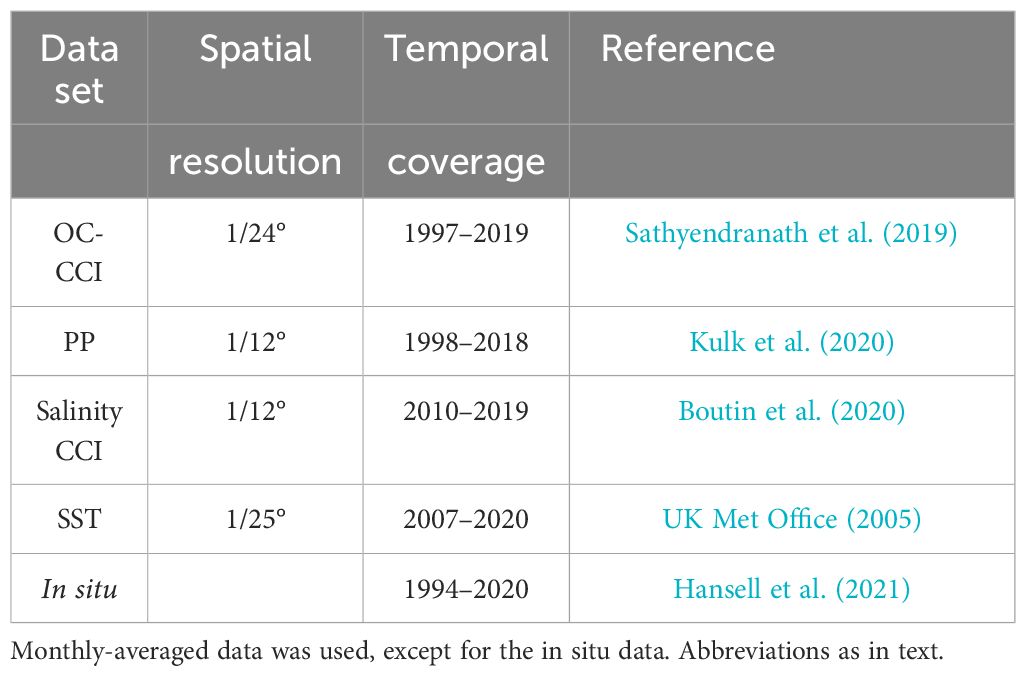
Table 1 Overview of the data sets used in this study.

OSTIA foundation SST (UK Met Office, 2005; Fiedler et al., 2019). All data was obtained at ∼9 km (1/12°) or better spatial resolution – or reprojected to that resolution – and monthly temporal resolution. Figure 1 shows examples of the global satellite data sets for June 2018.

Figure 1

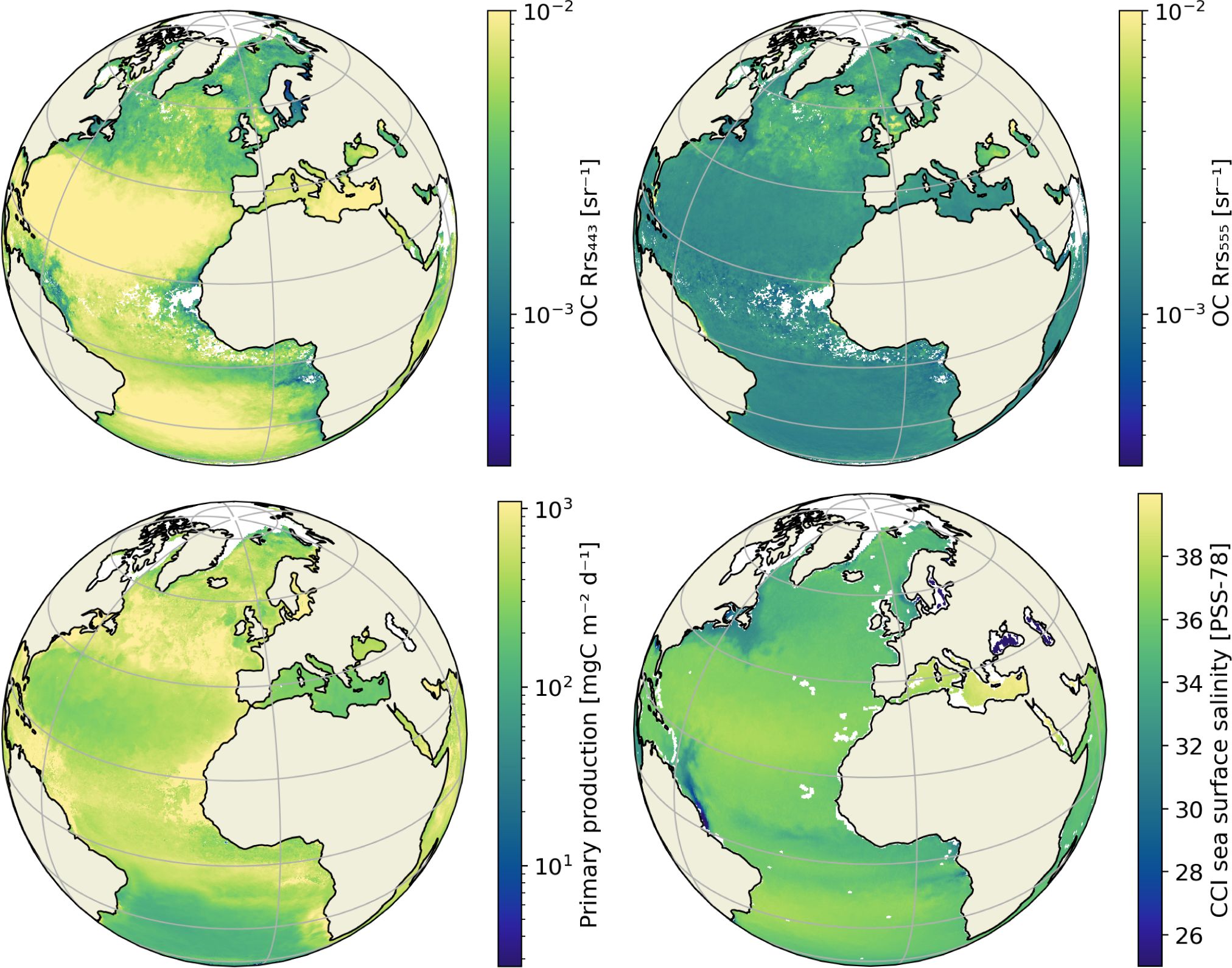
Figure 1 Examples of the satellite datasets with. Top left: the remote sensing reflectance (Rrs) at 443 nm. Top right: Rrs at 555 nm. Bottom left: primary production. Bottom right: sea surface salinity. All represent June 2018 mean values. Rrs and primary production are given in log scale. Light grey areas over the oceans are missing data.

2.2 In situ data

To train the global DOC model, i.e. to calibrate the model parameters, and validate model predictions, in situ DOC observations were used (Table 1). The global in situ data set from Hansell et al. (2021) (1994– 2020) was used, which include DOC concentrations and ancillary data from different field campaigns worldwide (Figure 2). From these datasets, we removed any duplicates, and we selected those in situ observations where the concentration of DOC was reported and its value was greater than zero. In addition, we chose only near surface measurements, with criteria ‘CTD PRESSURE’ ≤ 30 dbar, corresponding approximately to 30 metres.

Figure 2

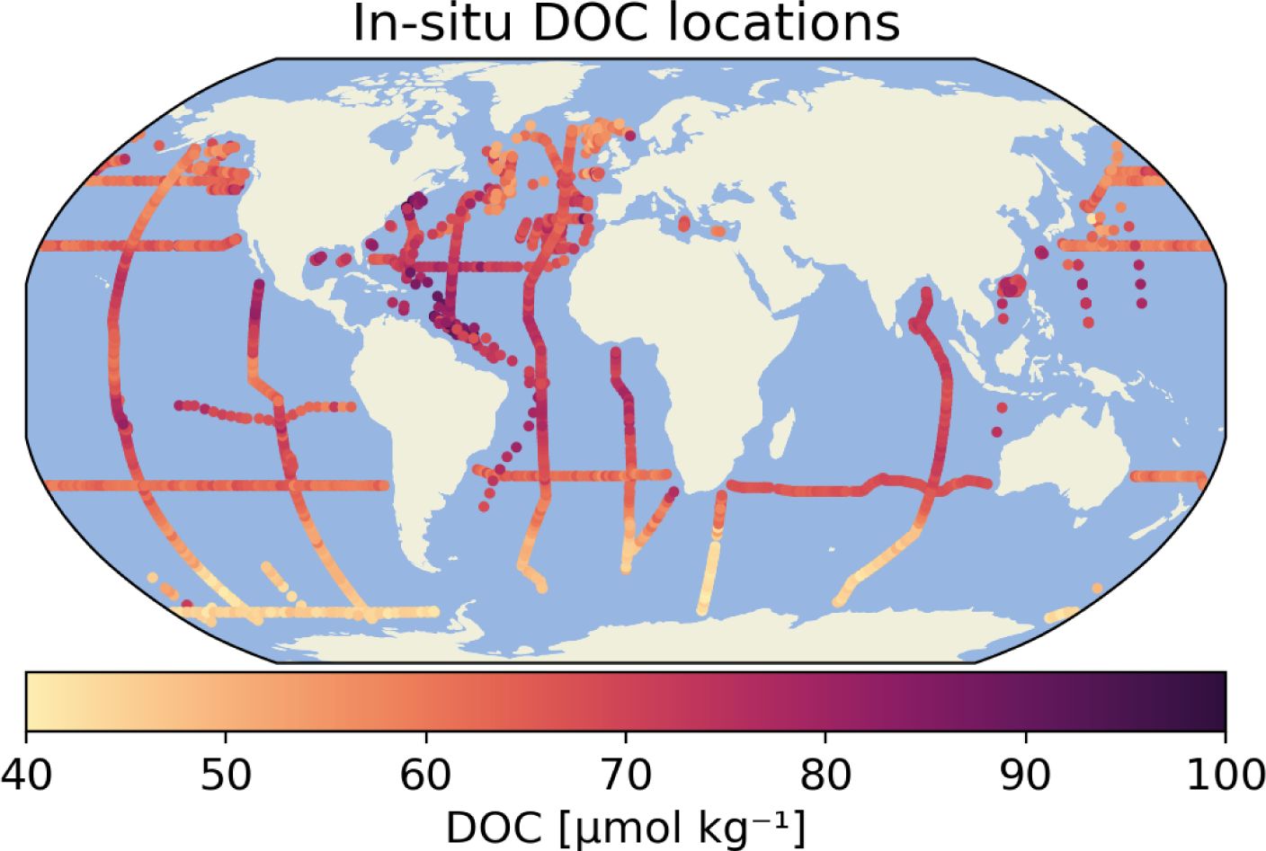
Figure 2 Locations of the in situ Dissolved Organic Carbon measurements, collected around the world on various field campaigns (Hansell et al., 2021). The original data have been aggregated to monthly means in 1/24° x 1/24° grid boxes.

After data selection of near-surface in situ DOC, we had a total of 12,910 in situ observations available for further analysis. The in situ data was matched-up with the satellite data at the time and location of each in situ observation and a total of 8,796 data points were available for all regression variables, which forms the maximum size of the training data set for model calibration. However, we further decided to aggregate the in situ data to the same spatial and temporal resolutions as our monthly satellite data. After calculating monthly means and means over 1/24° spatial grid, we were left with 1,339 data points. We note that the overlapping period of in situ and satellite data is 2010–2018, as this is the time period for which sea surface salinity from CCI and the satellite-based primary production data were available.

2.3 Machine learning models

Linear regression and visual inspection of pair-wise correlation between variables was used to set a baseline for modelling of DOC using other machine learning methods and to make an initial selection of regression variables. The initial multiple linear regression model used here is similar to that of Aurin et al. (2018). We have a total of 13 candidate regressors to predict surface water DOC in μmol kg⁻¹. The regressors, or features in machine learning terminology, are listed in Table 2. As satellite derived quantities, we are using normalised remote-sensing reflectance at wavelength 412, 443, 490, 510, 555 and 670 nm from the OC-CCI as Rrs_nnn, primary production from Kulk et al. (2020) as PP. Other globally available regressors include sea surface temperature and salinity. The geographical variables used were water depth and distance to shore. All these regressors are available at the in situ locations together with the observed DOC to train the model to be used globally over the open ocean. For satellite-based data we used monthly averages interpolated to the location and time of in situ data. Scatter plots of in situ DOC vs. various regressors are given in the auxiliary material (Supplementary Figure 1).

Table 2

Table 2 Regressors used in the models.

For advanced machine learning we use random forest and gradient boosting algorithms. Both are ensemble machine learning methods that use random subsamples of the training data set and builds decision trees or regression models for each sample, with the final model being a combination of the individual models. The book by Murphy (2012) gives an introduction to both methods as well as other similar machine learning approaches. In this study, we have used the Python package scikit-learn (Pedregosa et al., 2011) and its functions LinearRegression, RandomForestRegressor and GradientBoostingRegressor as well as several feature selection and cross validation tools available in the package. To illustrate random forest, Figure 3 shows an example of what an individual decision tree might look like. The actual trees are usually much larger.

Figure 3

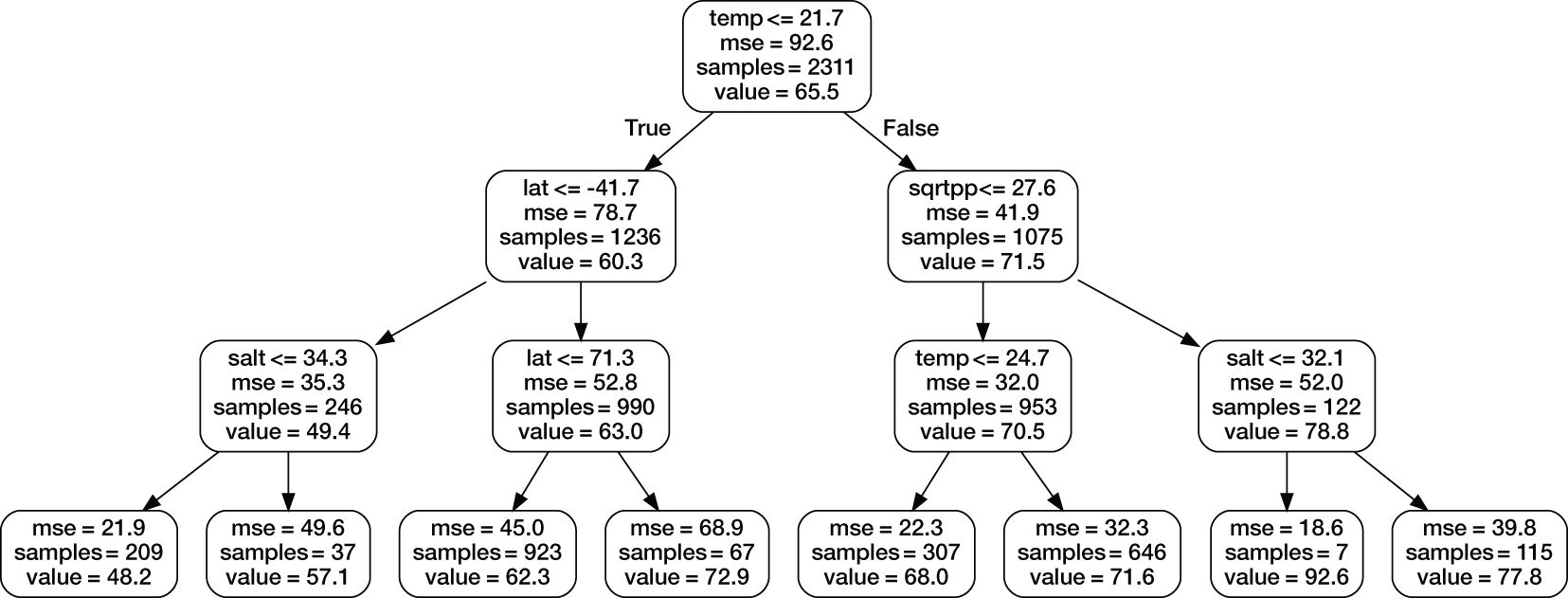
Figure 3 A simplified illustration of one random forest decision tree. The actual trees used in the model are much larger. The top line in each box shows branch selection criteria, “mse” is mean squared error in the test data set, “samples” is the size of the sample in the branch, and “value” is the estimated value of DOC.

2.4 Model and hyper-parameter selection

An important step in model building is the selection of explanatory variables. Including all or too many regressors will make the model perform better for the training data set, but typically causes over-fitting, i.e., the model is not able to predict beyond the data used in training. This is the reason why most machine leaning models use a separate and independent parts of the observational data to evaluate the model’s performance. Although there are automatic methods to select explanatory variables, or features, some hand-tuning is necessary. In the case of DOC, the amount of in situ data is still limited, both spatially and temporally (Figure 2).

We ended up comparing 6 models: multiple linear regression with full and reduced set of predictors, and random forest model and gradient boosting model with L2 (least squares) and L1 (least absolute deviation) optimisation criteria. The models use all available regressors given in Table 2, except for the reduced linear model, which used variables SST, $\sqrt{\text{PP}}$, Rrs₄₄₃, Rrs₅₁₀, Rrs₄₉₀, and Rrs₅₅₅, which were receiving largest Lasso scores when using L1 Lasso cross validation feature selection criteria available in the scikit-learn (Pedregosa et al., 2011) package (shown later in Figure 4).

Figure 4

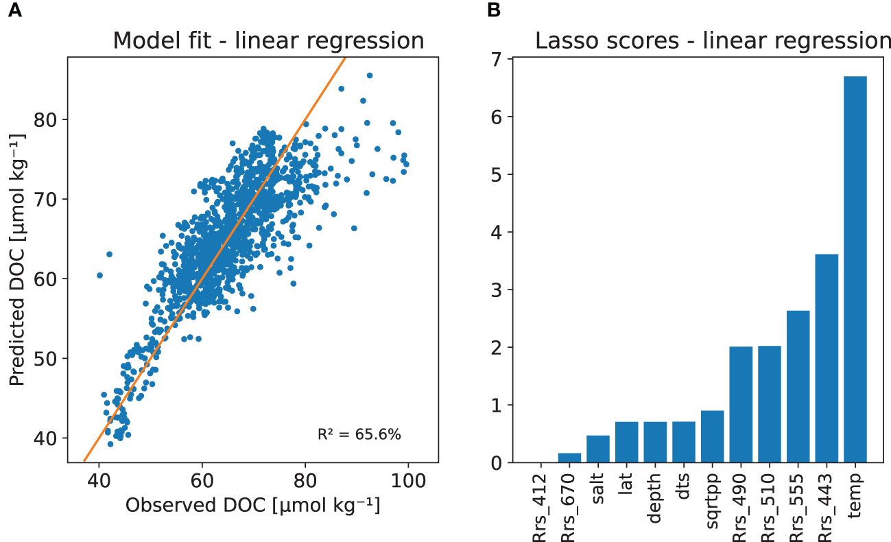
Figure 4 DOC multiple linear regression model with (A) Predicted versus observed Dissolved Organic Carbon (DOC) concentrations (in μmol kg⁻¹, and (B) LassoCV scores for the model parameters.

Tuning and verification of the DOC model is challenging due to relative small number of data points for building a global model that depends on seasonally varying covariates. Due to sequential nature of the in situ sampling (Figure 2), simple leave-one-out cross validation is not optimal, as even an over-fitted model will easily predict a data points that are very close in time and place to values used in training. Here we decided to do cross-validation and model hyper-parameter tuning by leaving out individual years of the training data and then predicting DOC at the in situ location of these left-out years. The main cross validation criteria used for model selection and tuning of the boosting algorithms was R² coefficient of determination of the prediction, called Q² in the following. Other cross validation criteria used were root mean squared error (RMSE) of prediction and mean absolute error (MAE) of prediction. For random forest and gradient boosting, the cross validation was performed 30 times to calculate the mean Q² and other criteria mentioned above. For the multiple linear regression model similar cross validation was performed 100 times. The optimisation was done using package Optuna (Akiba et al., 2019). The both machine learning regression models turned out to be quite robust to overfit. We found out that the best performance was achieved when allowing full model with all available predictors and letting the hyper-parameter optimisation algorithm tune the models using cross validated predictive ability. The three hyper-parameters that were tuned in the process were max_depth, n_estimators, and max_features (Pedregosa et al., 2011). The best performance was achieved by the random forest model and L1 criteria. Table 3 shows the result of model validation and comparison.

Table 3

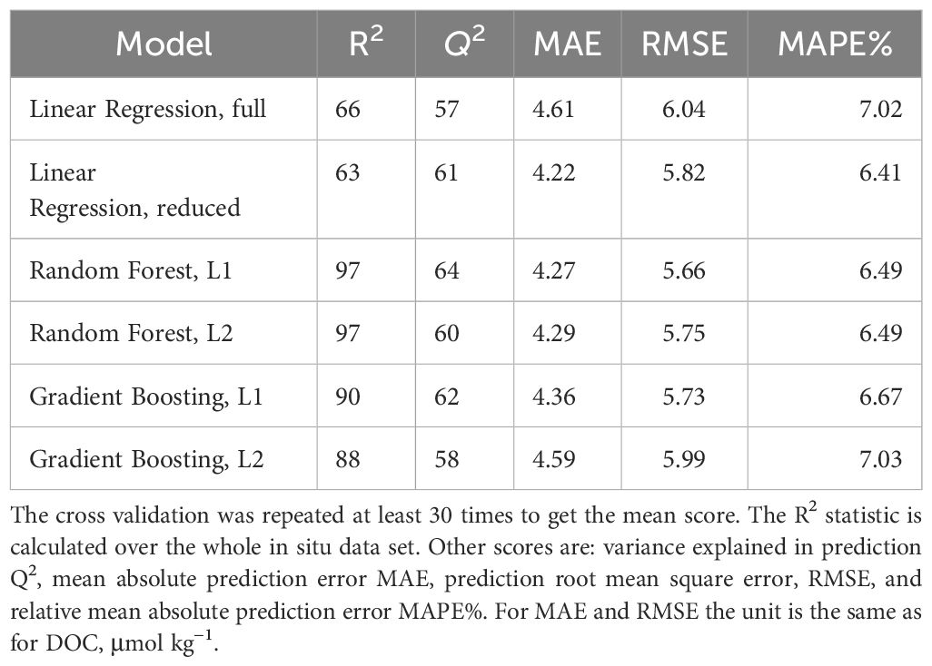
Table 3 Validation of different models using stratified cross validation.

In addition to the above cross validation based model tuning, we further evaluated the models using the same year-by-year cross validation as in the tuning, whose results are shown in Table 3. The results for two years, 2010 and 2011, are given in Figure 5, showing estimated vs. observed DOC for the given year with a model that is using all the years as well as cross-validation results where the year has been left out from the training set. Similar figures for all years are given in auxiliary material as Supplementary Figure 5. For the random forest model, the Q² values for prediction ranged from 20% to 77% for different years. This is an indication that the available training data might not be adequate, or at least that we do need to use all available data to be able to make reasonable predictions. However, the low values for some years in predictive variance explained is not only the property of random forest model. For the multiple linear regression models experimented, the yearly Q² values were much worse, also including negative values, which indicate that the linear model is performing worse in predicting new observations than just using the observed average.

Figure 5

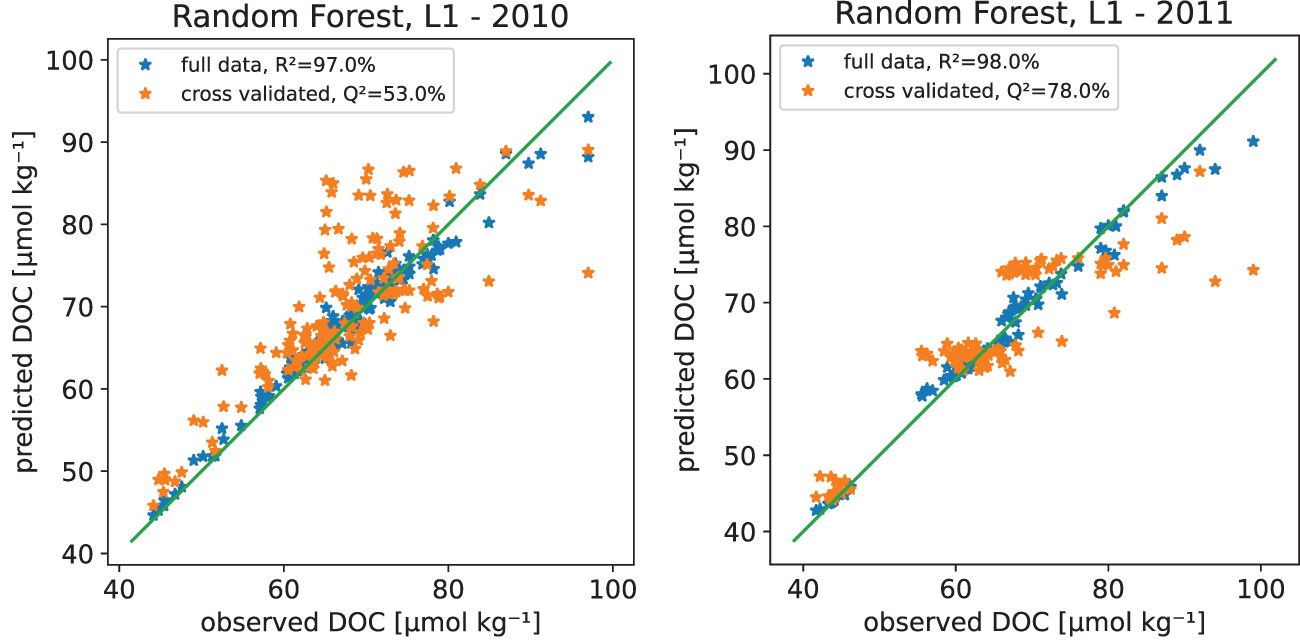
Figure 5 Observed versus predicted Dissolved Organic Carbon (DOC) in μmol kg⁻¹ from the random forest model in years 2010 and 2011 with the 1:1 line. The panel shows model fitted with all available data as well as the version where the given year has been left out of the training data set. All the estimated years are shown in Supplementary Figure 16 in the Supplementary Material.

2.5 Uncertainty in the predictions

The problem with many machine learning tools is that they do not provide uncertainty estimates for the predicted values. To estimate the predictive ability of the DOC random forest regression model and the uncertainty in predictions, we evaluated model residuals and their dependency on external variables, such as distance-to-shore and SST. In Figure 4 DOC estimations errors, i.e., the difference between in situ values and the corresponding model predicted values, are plotted against distance to shore. Panel on left shows absolute errors and panel on right shows relative errors interpolated spatially over the globe using regression kriging. Concentrations of DOC nearshore that are close to river and land discharges will be controlled heavily by factors that do not directly depend on the global variables available from space. For this reason, the data used for the DOC random forest model training include only those data points with distance-to-shore (e.g., variable dts) greater than 300 km. We chose this distance based on model performance and uncertainty analysis as described above. We note that the global predictions of DOC (section 3.2) are calculated also for near shore points where the accuracy is not optimal and only reflects the background DOC not affected by inland fluxes.

2.6 Other machine learning methods

There are other machine learning methods that have been used successfully when predicting natural phenomena. The use of artificial neural networks (ANN) has grown enormously in recent years and they have shown to have good performance in complicated modelling situations. An ANN model is even more dependent on good training data than the machine learning methods experimented here. We did experiment with ANN for DOC estimation, but at least with tests utilising dense network layer structure with different number of layers and layer widths, we were not able to build models that would have enough predictive performance with the Q² criteria. The full development of a neural network model, given the rapid development of the field in recent years, would need much more work than was available for this study. We refer to Bonelli et al. (2022) and earlier Roshan and DeVries (2017) for interesting experiments using ANN for modelling DOC.

3 Results

Figures 6, 7 show random forest and gradient boosting models fitted to the whole in situ training data set. Both models can provide very good fit to the whole in situ data and from the feature importance analysis we can infer that all the regressors used can provide some extra information to the procedure. The most important predictors being sea surface temperature and latitude of the observation. If we compare this to Figure 8 of multiple linear regression and Lasso cross validation based scores we see that the fit is much better and the effect of latitude is not so strong, which is natural as the effect is not linear on the value of the latitude. We could have tried to use different transformations to achieve linearity, so this comparison is not totally fair against a more simple model that only includes linear effects.

Figure 6

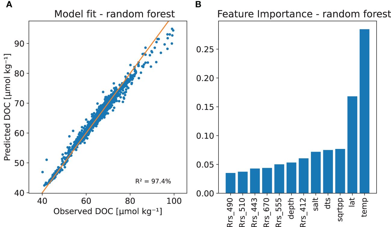
Figure 6 The DOC random forest model with (A) Model fit with the observed versus predicted DOC and (B) The relative importance of the regressor variables based on a permutation method.

Figure 7

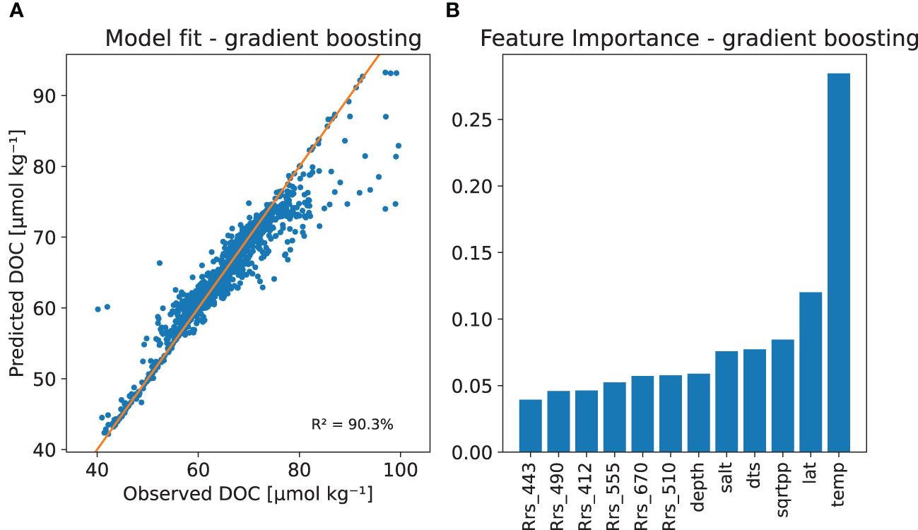
Figure 7 The DOC gradient boosting model with (A) Model fit with the observed versus predicted DOC and (B) The relative importance of the regressor variables based on a permutation method.

Figure 8

Figure 8 Uncertainty in the DOC random forest model. Left: the estimation error in all in situ locations compared against distance-to-shore. Right: the relative mean absolute error interpolated globally using regression kriging method and distance to shore as predictor. The dots show relative model residual error at in situ locations.

As seen in Figure 6A, the random forest DOC model can produce a good fit to the training data with an R² and Q² values of 97% and 64%, respectively (see Table 3). Variable importance, or feature importance in machine learning terminology, based on a permutation method, is shown in Figure 6B. The SST and latitude being the most important features. From ocean colour the reflectance at 412 nm was the most important, salinity and primary production bringing both about equally amount of predictive power to the model. There is a tendency to over-fit, but still we conclude, that machine learning DOC models provide relatively robust behaviour in cross validation. Supplementary Figure 3 in supplementary shows observed vs. predicted DOC scatter plots for individual years.

We used model residuals and their dependency on external variables to estimate the predictive ability of the model and the uncertainty in predictions. This analysis showed that a rough estimate of the relative uncertainty in the estimated DOC is on average 5% or less when in open ocean waters, i.e., more than 1,000 km from the shore, and the error stays smaller than 10% when the distance is more than 300 km, see Figure 4.

3.1 Validation against measurement sites

There are few open ocean stations that measure DOC in systematic manner. As an independent validation, we used in situ data from two sites. The first time series was obtained at the Hawaii Ocean Time-series HOT-DOGS application⁴. We compared model estimates to the in situ measurements from station Aloha (22°45’N, 158°W), which were not part of the data used in the model calibration. Figure 9 shows the estimated DOC with observations. In this case, all our global models show similar seasonal pattern that does not fully match to that in the observations. There is an average bias of 1–3 µmol kg⁻¹ for both machine learning models. The multiple linear regression model has larger bias. The seasonal pattern is not so noticeable in the observation, perhaps due to sampling and representation issues. Overall the match is quite good and within the anticipated estimation error.⁴

Figure 9

Figure 9 Time series from globally estimated DOC with gradient boosting and random forest models (both using L1 error criteria) and reduced linear regression model at a location of Aloha HOT-DOGS station compared to observations available from that stations for 2010–2018.

Figure 10 shows similar time series of data from Bermuda Atlantic Time-Series study (BATS, 31°40’N, 64°10’W) station. This is the same data set as was used by Bonelli et al. (2022), who kindly provided the data they used. We used daily averages of first 30 metres depth, whereas Bonelli et al. (2022) used 50 m. Here the observational data shows much clearer seasonal variability, which is also present in all the models. From year 2014, the variability of the observation changes, again perhaps due to some changes in sampling. The bias in the model results is up to 7% during some years. There were only three observations in Hansell et al. (2021) data set close to BATS that are used to train the model for years 2010–2018. Those are shown separately in the figure.

Figure 10

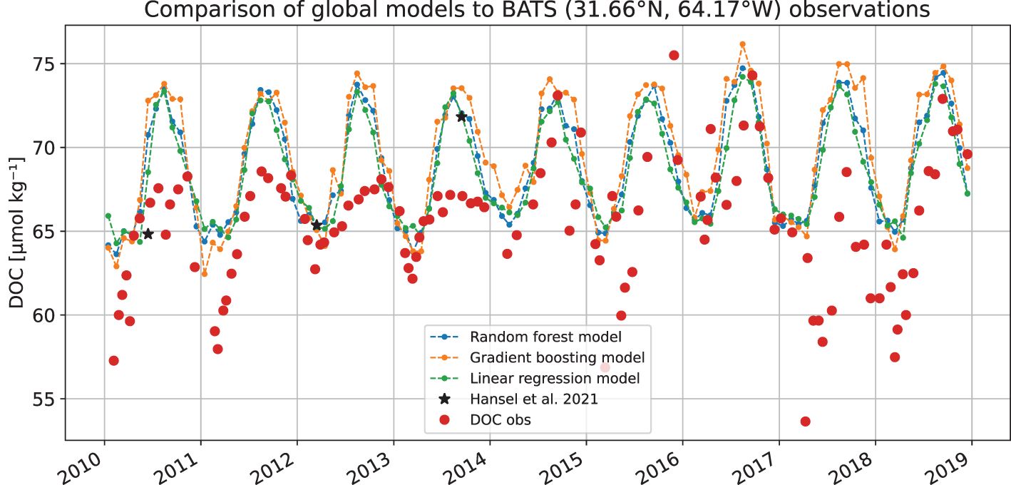
Figure 10 Time series from globally estimated DOC with gradient boosting and random forest models (both using L1 error criteria) and reduced linear regression model at a location of BATS station compared to observations available from that stations for 2010–2018.

3.2 Global satellite-based DOC time series

Using our DOC model for open water, we generated a global monthly time series of DOC for 2010– 2018, for which time period, all global input data were available. The output data have a spatial resolution of 9 km (1/12°) in an uniform longitude-latitude grid, and the data contains the estimated monthly DOC concentrations in μmol kg⁻¹. Data were generated only for those locations where remote sensing reflectance, primary production, salinity and SST data were available. We used the open ocean model even for near shore pixels. As examples, Figure 11 shows the mean climatology for years (2010–2018), with more maps provided in the supplementary material (Supplementary Figure 4). The entire data set is freely available online through the UK Centre for Environmental Data Analysis (CEDA).

Figure 11

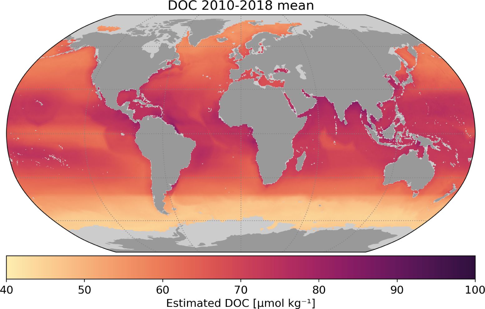
Figure 11 Climatology of Dissolved Organic Carbon (DOC) for 2010–2018. The light grey areas represent missing pixels for which input satellite data from CCI was not available. Climatologies of each year in the time series are provided in the Supplementary Material.

4 Discussion

Thanks to the comprehensive collections of in situ DOC data by (Hansell et al., 2021), it is now possible to apply machine-learning-based methods to estimate DOC in the surface waters of the global ocean. This is, nevertheless, a challenging task (Brewin et al., 2021). The current work explored modelling surface DOC from satellite data using multiple linear regression, gradient boosting and random forest. They are all designed to map the output variable of interest from the input variables in such a way that the model would have some explanatory power on predicting values outside the training data set. Extended validation of the models is still essential to establish confidence in the model predictions. This study shows that there are promising possibilities, but also room for more work.

In this study, we presented a machine learning approach to develop a global time series of DOC from observations of remote-sensing reflectance values at OC_CCI provided wavelengths (412, 443, 490, 510, 555, and 670 nm) phytoplankton primary production, sea surface temperature and salinity, as well as geographical variables. Other studies have used similar predictor variables, notably sea surface temperature and salinity, but also other variables such as nutrient concentrations and the absorption of Colour Dissolved Organic Matter (a_CDOM) (Siegel et al., 2002; Roshan and DeVries, 2017; Aurin et al., 2018; Bonelli et al., 2022). The selection of predictor variables is in part driven by domain-knowledge, but also by the type of data available. We have chosen to use only those predictor variables that are available from remote sensing observations, while other studies have used a combination of data available from in situ observations, satellite observations and biogeochemical models (Siegel et al., 2002; Aurin et al., 2018; Bonelli et al., 2022). In the DOC model presented here, sea surface temperature and latitude had the highest relative importance in predicting DOC, followed by primary production, distance to shore, sea surface salinity, and the remote sensing reflectance at 412 nm, (Figure 6). The importance of temperature and salinity in estimating DOC has been demonstrated in other studies: for example, the empirical model of Siegel et al. (2002) is based on relationships between temperature and in situ DOC that are parameterised per ocean basin; and the empirical model of Aurin et al. (2018) is based on the relationship between sea surface salinity and satellite-derived a_CDOM. While phytoplankton biomass has been used in other global DOC models (Roshan and DeVries, 2017; Bonelli et al., 2022), phytoplankton primary production is not commonly used, maybe in part because in situ observations of primary production are not available in sufficient numbers. Here, satellite-based primary production is seen to add to the predictive power of the gradient boosting and random forest models. It is important that internally consistent datasets based on the Ocean Colour Climate Change Initiative (remote sensing reflectances and primary production) were used in this study.

The DOC values estimated from our model compared well with in situ observations used in training the model (Figure 6). Leave-one-year-out cross validation (Figure 5) showed varying consistency across the years, but still provided reasonable results. Distance from shore (dts) appeared as a key determinant of outliers (Figure 4). Validation against in-situ measurements at Station Aloha and at BATS (Section 3.1) revealed biases that were in agreement with the assumed errors, and also showed challenges in reproducing seasonal variability at a local scale. The globally-mapped climatology (Figure 11) can be compared visually with the results of Bonelli et al. (2022), who recently published a 10-year DOC climatology based on a neural network approach that incorporated sea surface temperature, absorption of CDOM and chlorophyll-a. The two models showed a high level of qualitative agreement in spite of the differences in the AI methods employed, and in the satellite input data sets used. Though we did not use absorption by CDOM in our analysis, it is interesting to note that one of the key regressor variables in our study is the remote-sensing reflectance at 412 nm, the wavelength were the absorption by CDOM is the highest, compared with longer wavelengths that were included in the model.

All the tested machine learning models suffer from the tendency to over-fit. Their ability to model and find non-linear relationships between explanatory variables and the variable of interests (DOC in our case) is their strength. At the same time, it can be a weakness, if not enough representative in situ and satellite observations are used. The validation of predictions by independent observations is not always possible and the second best option is to cross validate by leaving out a part of the already scarce data. Doing cross validation and studying errors in the predictions can also help on the second problematic feature of many machine learning models, namely the lack of uncertainty estimates in model outputs. The tested approaches showed similar performance. Machine learning models require careful tuning of the parameters of the methods as they are prone to perform well on the data set that is used for training the model, but have worse results on independent new data. The ability to predict new observations and extrapolate spatially and temporally is usually the main reason to use machine learning models. In our case having a single collection of in situ observations, the problem of over-fitting is handled by using model scoring based on repeated cross validation by stratified random sampling. The final results will necessarily have some dependency on the choice of model’s tuning parameters and other estimation strategies. This is a common feature in advanced machine learning models.

Against the background of the complex biogeochemistry of DOC and in the absence of a clear optical signal that can unequivocally be related to DOC, our study has focused on exploring indirect methods to estimate DOC using proxy variables selected on the basis of our understanding of the biogeochemistry of DOC. Using an in situ database and satellite observations of primary production, sea surface temperature and salinity as well as remote sensing reflectances, a series of empirical and machine-learning approaches were tested to map global DOC in open ocean waters. This resulted in the selection of a satellite-based random forest model to map the total pelagic DOC on a monthly basis between 2010–2018. Due to spatially and temporally limited in situ data, it is still unclear how well the model can represent the seasonal patterns and trends in the global ocean DOC. One future approach might be to include dynamical processes, such as advection by ocean currents in satellite-based DOC models to improve our understanding of the temporal dynamics and spatial correlation structures of DOC. Undoubtedly, further progress must rely on parallel improvement in our understanding of the biogeochemical processes that underpin DOC dynamics in the ocean, as well as in improvements to the in situ data on DOC, with respect to both geographical and seasonal coverage.

Data availability statement

The datasets presented in this study can be found in online repositories. The names of the repository/repositories and accession number(s) can be found below: https://catalogue.ceda.ac.uk/uuid/372375fff81e44428ed62dacd562a5f2.⁵. The code used in the analysis is available from https://github.com/mjlaine/ESA-BICEP-DOC which is now public repository.

Author contributions

ML: Methodology, Software, Visualization, Writing – original draft, Writing – review & editing. GK: Methodology, Visualization, Writing – review & editing. BJ: Conceptualization, Data curation, Software, Writing – review & editing. SS: Conceptualization, Funding acquisition, Project administration, Resources, Supervision, Validation, Writing – review & editing.

Funding

The author(s) declare financial support was received for the research, authorship, and/or publication of this article. This research was funded by European Space Agency’s project BICEP - Biological Pump and Carbon Exchange Processes and the Simons Foundation grant Computational Biogeochemical Modeling of Marine Ecosystems (CBIOMES, number 549947, SS). ML was partly supported by Research Council of Finland grant n:o 321890. This work is a contribution to the activities of the National Centre of Earth Observation of the UK.

Acknowledgments

We would like to thank Ana Bonelli for providing details of her analysis of the time series data at BATS, for comparison with the results presented in this study.

Conflict of interest

The authors declare that the research was conducted in the absence of any commercial or financial relationships that could be construed as a potential conflict of interest.

The author(s) declared that they were an editorial board member of Frontiers, at the time of submission. This had no impact on the peer review process and the final decision.

Publisher’s note

All claims expressed in this article are solely those of the authors and do not necessarily represent those of their affiliated organizations, or those of the publisher, the editors and the reviewers. Any product that may be evaluated in this article, or claim that may be made by its manufacturer, is not guaranteed or endorsed by the publisher.

Supplementary material

The Supplementary Material for this article can be found online at: https://www.frontiersin.org/articles/10.3389/fmars.2024.1305050/full#supplementary-material

Footnotes

1. ^ https://catalogue.ceda.ac.uk/uuid/99348189bd33459cbd597a58c30d8d10
2. ^ https://dx.doi.org/10.5285/69b2c9c6c4714517ba10dab3515e4ee6
3. ^ https://catalogue.ceda.ac.uk/uuid/7813eb75a131474a8d908f69c716b031
4. ^ University of Hawai’i at Mānoa. National Science Foundation Award # 1756517 https://hahana.soest.hawaii.edu/hot/hot-dogs/bextraction.html
5. ^ https://catalogue.ceda.ac.uk/uuid/372375fff81e44428ed62dacd562a5f2

References

Akiba T., Sano S., Yanase T., Ohta T., Koyama M. (2019). “Optuna: A next-generation hyperparameter optimization framework,” in Proceedings of the 25th ACM SIGKDD International Conference on Knowledge Discovery and Data Mining. (New York, NY, USA: Association for Computing Machinery), 2623–2631. doi: 10.1145/3292500

CrossRef Full Text | Google Scholar

Aurin D., Mannino A., Lary D. J. (2018). Remote sensing of CDOM, CDOM spectral slope, and dissolved organic carbon in the global ocean. Appl. Sci. 8. doi: 10.3390/app8122687

CrossRef Full Text | Google Scholar

Bonelli A. G., Loisel H., Jorge D. S. F., Mangin A. (2022). Odile Fanton d’Andon, and Vincent Vantrepotte. A new method to estimate the dissolved organic carbon concentration from remote sensing in the global open ocean. Remote Sens. Environ. 281, 113227. doi: 10.1016/j.rse.2022.113227

CrossRef Full Text | Google Scholar

Boutin J., Vergely J.-L., Reul N., Catany R., Koehler J., Martin A., et al. (2020) ESA Sea Surface Salinity Climate Change Initiative (Sea_Surface_Salinity_cci): Monthly sea surface salinity product, v2.31, for 2010 to 2019. Available at: https://catalogue.ceda.ac.uk/uuid/7813eb75a131474a8d908f69c716b031.

Google Scholar

Brewin R. J. W., Sathyendranath S., Müller D., Brockmann C., Deschamps P. Y., Devred E., et al. (2015). The ocean colour climate change initiative: Iii. a round-robin comparison on in-water bio-optical algorithms. Remote Sens. Environ. 162, 271–294. doi: 10.1016/j.rse.2013.09.016

CrossRef Full Text | Google Scholar

Brewin R. J. W., Sathyendranath S., Platt T., Bouman H., Ciavatta S., Dall’Olmo G., et al. (2021). Sensing the ocean biological carbon pump from space: A review of capabilities, concepts, research gaps and future developments. Earth-Science Rev. 217, 103604. doi: 10.1016/j.earscirev.2021.103604

CrossRef Full Text | Google Scholar

Fichot C. G., Benner R. (2012). The spectral slope coefficient of chromophoric dissolved organic matter (s275–295) as a tracer of terrigenous dissolved organic carbon in river-influenced ocean margins. Limnol. Oceanogr. 57, 453–1466. doi: 10.4319/lo.2012.57.5.1453

CrossRef Full Text | Google Scholar

Fiedler E. K., McLaren A., Banzon V., Brasnett B., Ishizaki S., Kennedy J., et al. (2019). Intercomparison of long-term sea surface temperature analyses using the GHRSST multi-product ensemble (GMPE) system. Remote Sens. Environ. 222, 18–33. doi: 10.1016/j.rse.2018.12.015

CrossRef Full Text | Google Scholar

Hansell D. A., Carlson C. A. (2013). Localized refractory dissolved organic carbon sinks in the deep ocean. Global Biogeochemical Cycles 27, 705–710. doi: 10.1002/gbc.20067

CrossRef Full Text | Google Scholar

Hansell D. A., Carlson C. A., Repeta D. J., Schlitzer R. (2009). Dissolved organic matter in the ocean: A controversy stimulates new insights. Oceanography 22, 202–211. doi: 10.5670/oceanog.2009.109

CrossRef Full Text | Google Scholar

Hansell D. A., Carlson R. M.W., Amon C. A., Álvarez-Salgado X. Antón, Yamashita Y., Romera-Castillo C., et al. (2021). Compilation of dissolved organic matter (DOM) data obtained from the global ocean surveys from 1994 to 2020 (NCEI accession 0227166). doi: 10.25921/s4f4-ye35

CrossRef Full Text | Google Scholar

Kulk G., Platt T., Dingle J., Jackson T., Jönsson B. F., Bouman H. A., et al. (2020). Primary production, an index of climate change in the ocean: Satellite-based estimates over two decades. Remote Sens. 12. doi: 10.3390/rs12050826

CrossRef Full Text | Google Scholar

Loisel H., Vantrepotte V., Dessailly D., Meriaux X. (2014). Assessment of the colored dissolved organic matter in coastal waters from ocean color remote sensing. Opt. Express 22, 13109. doi: 10.1364/OE.22.013109

PubMed Abstract | CrossRef Full Text | Google Scholar

Mannino A., Novak M. G., Hooker S. B., Hyde K., Aurin D. (2014). Algorithm development and validation of cdom properties for estuarine and continental shelf waters along the northeastern us coast. Remote Senssing Environ. 152, 567–602. doi: 10.1016/j.rse.2014.06.027

CrossRef Full Text | Google Scholar

Mannino A., Russ M. E., Hooker S. B. (2008). Algorithm development and validation for satellite-derived distributions of DOC and CDOM in the U.S. Middle Atlantic Bight. J. Geophysical Res.: Oceans 113. doi: 10.1029/2007JC004493

CrossRef Full Text | Google Scholar

Matsuoka A., Boss E., Babin M., Karp-Boss L., Hafez M., Chekalyuk A., et al. (2017). Pan-arctic optical characteristics of colored dissolved organic matter: Tracing dissolved organiccarboninchangingarcticwatersusingsatelliteoceancolordata. RemoteSensingofEnvironment 200, 89–101. doi: 10.1016/J.RSE.2017.08.009

CrossRef Full Text | Google Scholar

Murphy K. P. (2012). Machine Learning A Probabilistic Perspective (Cambridge, MA: The MIT Press). Available at: https://probml.github.io/pml-book/book0.html.

Google Scholar

Nelson N. B., Siegel D. A. (2013). The global distribution and dynamics of chromophoric dissolved organic matter. Annu. Rev. Mar. Sci. 5, 20.1–20.3. doi: 10.1146/annurev-marine-120710-100751

CrossRef Full Text | Google Scholar

Pedregosa F., Varoquaux G., Gramfort A., Michel V., Thirion B., Grisel O., et al. (2011). Scikit-learn: machine learning in python. J. Mach. Learn. Res. 12, 2825–2830. Available at: http://jmlr.org/papers/v12/pedregosa11a.html.

Google Scholar

Roshan S., DeVries T. (2017). Efficient dissolved organic carbon production and export in the oligotrophic ocean. Nat. Commun. 8, 2036. doi: 10.1038/s41467-017-02227-3

PubMed Abstract | CrossRef Full Text | Google Scholar

Sathyendranath S., Brewin R. J. W., Brockmann C., Brotas V., Calton B., Chuprin A., et al. (2019). An ocean-colour time series for use in climate studies: The experience of the Ocean-Colour Climate Change Initiative (OC-CCI). Sensors 19. doi: 10.3390/s19194285

CrossRef Full Text | Google Scholar

Siegel D. A., Behrenfeld M. J., Maritorena S., McClain C. R., Antoine D., Bailey S. W., et al. (2013). Regional to global assessments of phytoplankton dynamics from the SeaWiFS mission. Remote Senssing Environ. 135, 77–91. doi: 10.1016/j.rse.2013.03.025

CrossRef Full Text | Google Scholar

Siegel D. A., Maritorena S., Nelson N. B., Hansell D. A., Lorenzi-Kayser M. (2002). Global distribution and dynamics of colored dissolved and detrital organic materials. J. Geophys. Res. Oceans 107, 1–14. doi: 10.1029/2001JC000965

CrossRef Full Text | Google Scholar

UK Met Office (2005) GHRSST Level 4 OSTIA global foundation sea surface temperature analysis.doi: 10.5067/GHOST-4FK01.

CrossRef Full Text | Google Scholar

Williams P. M., Druffel E. R.M. (1987). Radiocarbon in dissolved organic matter in the central North Pacific Ocean. Nature 330, 246–248. doi: 10.1038/330246a0

CrossRef Full Text | Google Scholar