A learnable full-frequency transformer dual generative adversarial network for underwater image enhancement

1 Introduction

Underwater image enhancement is a complex and challenging endeavor aimed at enhancing the visual quality of underwater images to suit specific application scenarios. This technology finds extensive utility in domains like marine scientific research, underwater robotics, and underwater object recognition. Owing to the unique characteristics of the underwater environment, underwater images typically suffer from significant noise and color deviation, adding to the complexity of the enhancement process. Consequently, enhancing the quality of underwater images remains a daunting task, necessitating ongoing exploration and innovation to cater to the demands for high-quality underwater imagery across diverse application scenarios.

Traditional methods for underwater image enhancement often rely on manually designed features and shallow learning algorithms, which struggle to handle the inherent variability and complexity of underwater images. To tackle these challenges, recent research has shifted towards leveraging advanced deep learning techniques to enhance underwater image quality performance. Deep neural networks (Zhang et al., 2021a; Li et al., 2022) have exhibited remarkable capabilities in learning intricate patterns and representations directly from raw data, enabling them to adapt to the degraded and noisy nature of underwater images. One approach involves the direct development of complex deep network models, where researchers aim to create intricate deep structures to enhance underwater image quality. However, this approach often leads to issues of high model complexity. Another strategy explores leveraging characteristics from other domains to enhance images. This method allows for better processing of image details, structure, and frequency information, thereby improving clarity, contrast, and overall image quality. Although these methods have made strides in image enhancement, they sometimes overlook local feature differences. As illustrated in Figure 1, frequency domain techniques are employed to investigate the issue of perceptual quality distortion in degraded underwater images alongside their corresponding authentic reference images. The task of image enhancement is carried out by computing the one-dimensional power spectrum information (indicative of image information quantity) between the images. This involves an analysis of frequency domain variability across the images. Upon closer examination of different stages depicted in the figure, it is evident that there exists a discernible variance in the frequency domain power spectrum values between the original underwater image and the reference image at each stage, as presented across the entire frequency spectrum. Hence, employing a frequency domain decoupling method to separately learn and approximate the authentic labels proves to be a highly rational approach. By addressing these challenges, researchers can pave the way for more effective underwater image enhancement techniques, meeting the demands of various application scenarios effectively.

Figure 1

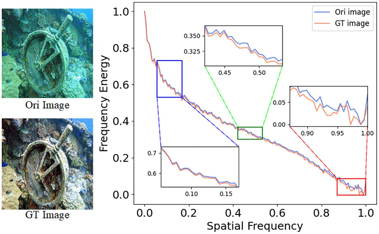
Figure 1 Frequency domain difference analysis between the original image and the ground-truth image, with the amount of image information represented as a 1D power spectral density image. The calculation method of 1D power spectrum image can be found in Appendix 1.1.

To cope with the above problems, we propose a novel underwater image enhancement method using the learnable full-frequency transformer dual generative adversarial network (LFT-DGAN). Specifically, we first design an image frequency domain decomposition without natural information loss based on a reversible convolutional neural network structure. Reversible convolutional networks allow us to apply the advantageous high-frequency texture enhancement approach explicitly and separately to the high-frequency branch, which greatly alleviates the problem of frequency conflicts in the optimization objective. In addition, an interactive transformer structure has been designed to ensure improved information consistency and interactivity across multiple frequency bands. Finally, we develop an efficient and robust dual-domain discriminator to further ensure high-quality underwater image generation. The main innovations of this article are as follows:

1. We present a novel approach to image frequency domain decomposition, implemented using reversible neural networks. This marks the first instance of introducing reversible neural networks to the domain of underwater image frequency domain decomposition.

2. We introduce an interactive transformer structure to ensure improved information consistency and interactivity across multiple frequency bands, further enhancing the quality of enhanced underwater images.

3. We have developed an efficient and robust dual-domain discriminator to further ensure high-quality underwater image generation. The proposed discriminator effectively distinguishes between real and generated images in both spatial and frequency domains, thereby aiding in achieving high-quality image enhancement results.

4. In comparison to current state-of-the-art methods, our approach yields satisfactory image effects across multiple underwater datasets. Additionally, we have performed several challenging applications, such as underwater image structure analysis, fog removal, and rain removal, demonstrating the superiority of our method.

2 Related work

2.1 Underwater image enhancement methods

The development of underwater image enhancement methods has evolved from the traditional methods at the beginning to deep learning methods, which have received much attention from scholars. Traditional underwater image enhancement methods are mainly based on the redistribution of pixel intensities to improve image contrast and color without considering the specific characteristics of underwater images. It mainly includes spatial domain and transform domain image enhancement; spatial domain image enhancement is primarily based on gray mapping theory, and intensity histogram redistribution is achieved by expanding the gray level, which is done in different color models, such as the retinex theory (Zhang et al., 2022a) and histogram methods (Ghani and Isa, 2017). Transform domain image enhancement generally transforms the image into the frequency domain, enhancing the high-frequency components (target edges) and eliminating the low-frequency components (background) to improve the quality of underwater images, such as Laplacian pyramid (Zhuang et al., 2022) and wavelet transform (Ma and Oh, 2022). These traditional underwater image enhancement methods have the advantages of high flexibility and low computational requirements; however, the traditional methods require human intervention, have limited enhancement effects, and lack generalization (they cannot be applied to multi-scene underwater scenes).

With the rapid development of deep learning, many new methods for underwater image enhancement have made significant progress and overcome some limitations of traditional methods. For example, Wang et al. (2021) effectively integrate RGB color space and HSV color space into a single CNN model and propose the uiec2-net end-to-end trainable network, which achieves better results in underwater images, but the authors are limited to the spatial domain and do not explore whether the transform domain could also effectively improve underwater image enhancement. To validate this idea, Wang et al. (2022b) use an asymptotic frequency domain module and a convolutional bootstrap module to create an underwater image correction model. However, the aforementioned deep learning methods often require a large amount of running memory and computational resources, which is not conducive to real-time application on underwater devices. In order to reduce the number of parameters and improve computational efficiency, Zheng et al. (2023) propose a lightweight multi-scale underwater enhancement model. They achieve efficient underwater image enhancement by using a layer-wise attention mechanism and a compact network structure. In addition to these methods, scholars have proposed GAN algorithms to improve the quality of image perception for underwater image enhancement. Wang et al. (2023a) enhance underwater images by integrating a cascaded dense channel attention module and a position attention module into the generator in the GAN framework. Li et al. (2018b) use a circular structure to learn the mapping function between input and target and propose a weakly supervised method for color correction of underwater images. Although the above methods achieve promising results, their performance is dependent on the network architecture design and training data, and deep learning architectures for underwater images have some potential drawbacks, such as limited applicability of the trained model, blurring of some underwater image features, and over-emphasis on human visual quality.

2.2 Image decomposition methods

Underwater images mainly suffer from color distortion caused by light absorption and blurring caused by light scattering (Wang et al., 2023b). In terms of spatial domain, image enhancement is generally performed as a whole, ignoring the coherence between multiple degradations. Image decomposition methods can help represent an image as a collection of frequency components, such as wavelet transform and sparse representation. By processing these frequency components, we can gain a better understanding of the structure and features of the image, and isolate noise and blur components. This decomposition method can assist with enhancing underwater images by addressing various degradation issues. Kang et al. (2022) decompose underwater images into three conceptually independent components of average intensity, contrast and structure for processing, and fusion to produce enhanced underwater images. Wu et al. (2021) decompose the underwater image into high- and low-frequency images, then process the high-frequency part using a deep learning method and the low-frequency part using a physical modeling method, and finally obtained the enhanced image.

Currently, the commonly used frequency domain decomposition methods include discrete Fourier transform (DFT), discrete wavelet transform (DWT), and discrete cosine transform (DCT). However, these methods are built based on mathematical approaches, which can cause different degrees of data loss phenomena and are not suitable for task-specific studies. For this reason, influenced by octave convolution (Chen et al., 2019), Li et al. (2021) use downsampling convolution to decompose mixed feature representations of images, and although they are able to decompose different frequency domain features, there is still unknown information loss due to the random loss of information features from convolution. In a similar operation, Jiang et al. (2023) use dilated convolution to decompose a mixed feature representation of the image, which also suffer from random loss of information (which could not be quantified). The above studies show that the convolution approach is effective in decomposing image information, so what is the best way to do it without information loss? The reversible convolution approach has the advantage of low memory and no loss of information. For this work, we can refer to the cornerstone NICE (Dinh et al., 2014), which describes the entire framework and coupling layers in detail. Although this method is widely used in the areas of image scaling (Xiao et al., 2020), denoising (Liu et al., 2021), and hiding information (Guan et al., 2022), it has not yet been explored in the area of underwater image decomposition. For this reason, we use a reversible convolution approach to decompose image information, which allows for both no loss of image information and a complete decomposition of the image hybrid feature representation.

3 Proposed method

The LFT-DGAN framework consists of a generator network and two discriminator networks. The generator takes underwater images as input and produces enhanced images. The two discriminator networks, one operating at the frequency level and the other at the image level, provide feedback to improve the quality of the generated images. The training process involves an adversarial loss, perceptual loss, l₁ loss, and gradient difference loss (GDL) to optimize the generator and discriminator networks, as shown in Figure 2.

Figure 2

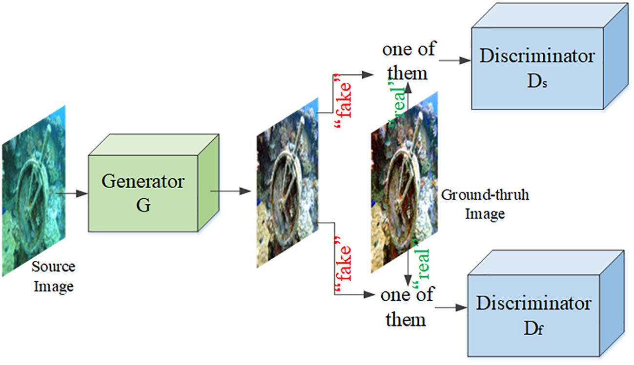
Figure 2 The overall network structure of LFT-DGAN, where D_s represents the image domain discriminator and D_f represents the frequency domain discriminator.

3.1 Generator network

The generator overall structure is shown in Figure 3. The network includes a frequency domain decomposition module and a frequency domain enhancement module. Specifically, given the original underwater image $\text{I} \in {\text{R}}^{\text{C}\times \text{H}\times \text{W}}$, our method first applies the frequency domain decomposition module to project the image into the low-frequency L₀, mid-frequency M₀, and high-frequency H₀ components’ (i.e., full-frequency) feature space, and then the low-frequency feature L₀ is used to extract the low-frequency effective feature L₁ through a multi-level residual network (ResBlk), while the mid-frequency feature M₀ and the feature L₁ go through an interactive transformer structure (LFT-ResBlk) to obtain the mid-frequency effective feature M₁. Subsequently, the effective mid-frequency feature M₁ and the high-frequency feature H₀ through the LFT-ResBlk obtain the high-frequency effective feature H₁. The effective high-frequency (H₁), mid-frequency (M₁), and low-frequency (L₁) features are further propagated into densely connected neural network modules to construct clear underwater images $\text{O} \in {\text{R}}^{\text{C}\times \text{H}\times \text{W}}$. The generator network process can be described as follows (Equations 1–5):

Figure 3

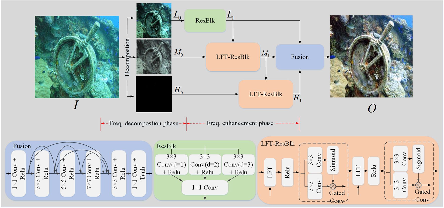
Figure 3 The generator framework of our proposed LFT-DGAN method. For detailed explanations of the Decomposition and LFT modules in the figure, please refer to Sections 3.1.1 and 3.1.2.

$\begin{array}{ll}{H}_0,M_0,L_0={\int }_d(I)& (1)\end{array}$

$\begin{array}{ll}{L}_1={\int }_{resblk}(L_0)& (2)\end{array}$

$\begin{array}{ll}{M}_1={\int }_{lft}(L_1,M_0)& (3)\end{array}$

$\begin{array}{ll}{H}_1={\int }_{lft}(M_1,H_0)& (4)\end{array}$

$\begin{array}{ll}O={\int }_{fusion}(L_1,M_1,H_1)& (5)\end{array}$

In the formula, ${\int }_d(·)$ represents the simplified forms of the frequency decomposition. ${\int }_{resblk}(·)$ signifies a multi-level residual network (ResBlk). ${\int }_{lft}(·)$ denotes an interactive transformer structure (LFT-ResBlk). ${\int }_{fusion}(·)$ refers to a densely connected fusion network.

3.1.1 Frequency decomposition module

In traditional signal processing methods, image transformation methods include fast Fourier transform (FFT), DCT, and DWT. These methods are deterministic mathematical operations and task-independent, and inevitably discard some key information for the recovery task. Both DFT and DCT characterize the entire spatial frequency domain of an image, which is not conducive to local information. DWT can represent the entire spatial frequency domain of an image and local spatial frequency domain features. In addition, scholars proposed dilated convolution filtering transform (DCFT) (Jiang et al., 2023) and up-/downsampling sampling filtering transform (USFT) (Li et al., 2021), both of which are difficult to measure quantitatively as the information through the convolution or up-/downsampling sampling will randomly lose high-frequency signals. Figures 4A–C show that different decomposition methods can separate low-, medium-, and high-frequency image differences to some extent, with the DWT being able to obtain better separation, while the convolution and up-/downsampling sampling filter transforms designed by the researcher are able to separate image differences in high-frequency images, and our proposed decomposition method can obtain better separation in each frequency domain. In addition, Figure 4D shows the low redundancy (correlation) of decomposed features by our proposed decomposition method, indicating that the image information is relatively thoroughly decomposed.

Figure 4

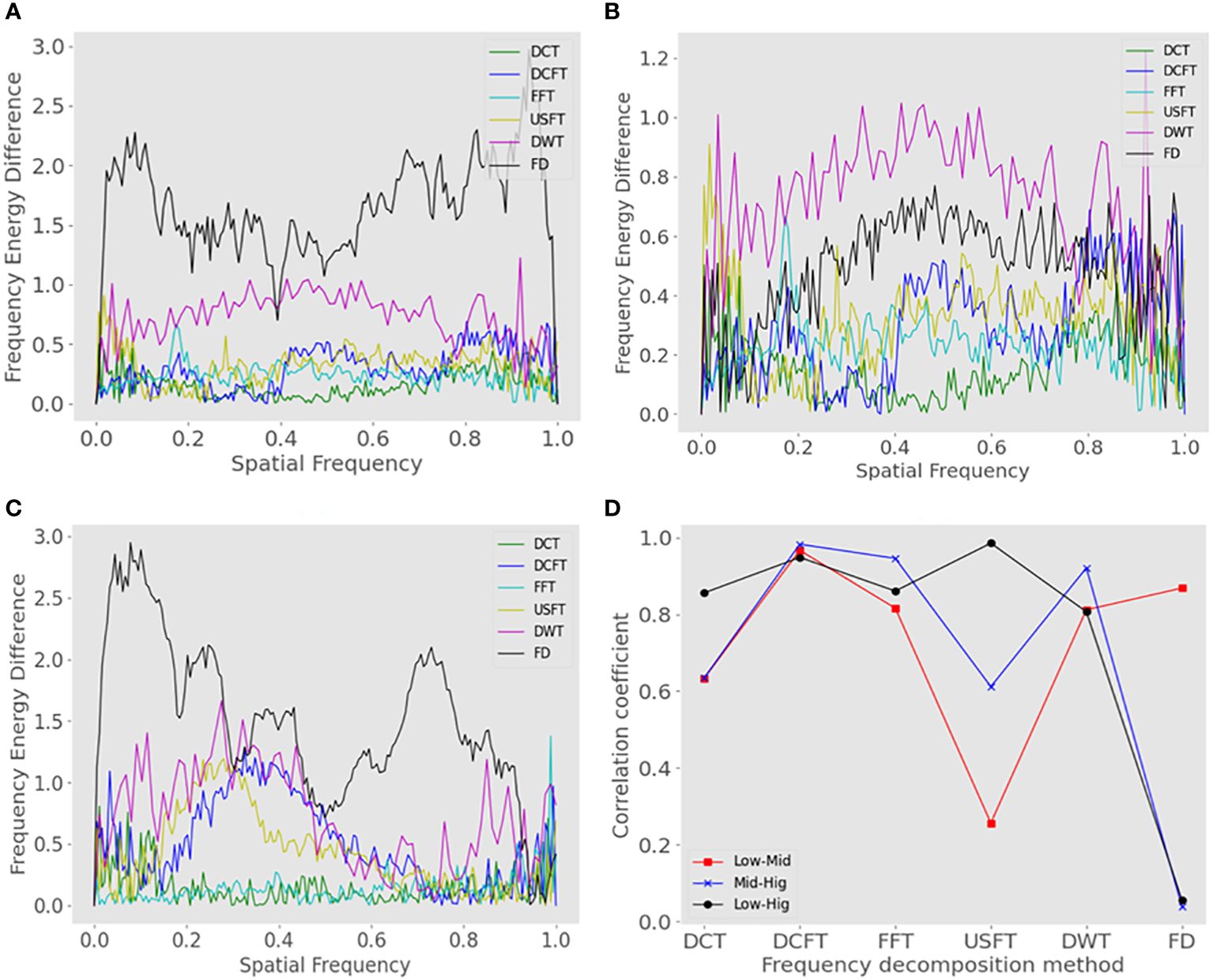
Figure 4 Analysis of the frequency domain difference between the original images (OI) and ground-truth images (GT) for different frequency domain decomposition methods. (A) Difference in the amount of low-frequency image information (1D power spectrum) between GT and OI. (B) Difference in the amount of information in the mid-frequency image between GT and OI. (C) Difference in the amount of high-frequency image information between GT and OI. (D) Correlation between low-, mid-, and high-frequency images for different frequency domain decomposition methods.

To solve the problems of information integrity and flexibility of decomposed images, we propose an image decomposition method based on reversible convolution. If we make the potential representation of the image after the reversible network transformation separable, the different frequency signals will be encoded in different channels. As shown in Figure 5, the input image goes through a reversible convolution module and produces two feature parts, Z₁ and Z₂. The Z₁ feature serves as the style extraction template for high-frequency features of the image. The Z₂ feature continues to pass through another reversible convolution module, resulting in Z₃ and Z₄. Similarly, the Z₄ feature acts as the style extraction template for medium-frequency features of the image. The Z₃ feature further goes through a reversible block to obtain the Z₅ feature, which is used as the style extraction template for low-frequency features of the image. Finally, based on the distribution of these new style templates, the original image is redistributed. This process decomposes the original image into high-, medium-, and low-frequency images, with each frequency part influenced by the corresponding style extraction template. Note that the reversible convolution module (Kingma and Dhariwal, 2018) uses the regular stream mode. The Frequency decomposition process can be described as follows (Equations 6–9):

Figure 5

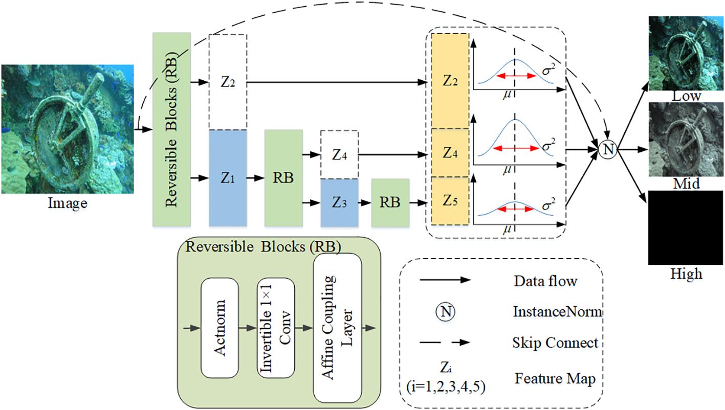
Figure 5 Image decomposition method based on reversible convolution.

$\begin{array}{ll}{Z}_1,Z_2=RB(I)& (6)\end{array}$

$\begin{array}{ll}{Z}_3,Z_4=RB(Z_2)& (7)\end{array}$

$\begin{array}{ll}{Z}_5=RB(Z_3)& (8)\end{array}$

$\begin{array}{ll}\text{low},\text{mid},\text{high}=[Z_2☉I,Z_4☉I,Z_5☉I]& (9)\end{array}$

where RB represents the reversible block. ☉ indicates the re-editing of images according to the new distribution.

3.1.2 Learnable full-frequency adaptive transformer

There are two key problems with the frequency domain hierarchical feature processing approach: (1) The amount of information in the low-frequency, mid-frequency, and high-frequency image features is significantly different, and a simple connection will greatly suppress the high-frequency information.

(2) Different branch enhancement modules will generate what they consider reasonable for their own bands (independent) and may not be consistent with other branch band enhancement content. To address these issues, we have designed a novel custom transformer structure technique that results in more realistic restoration results, as shown in Figure 6.

Figure 6

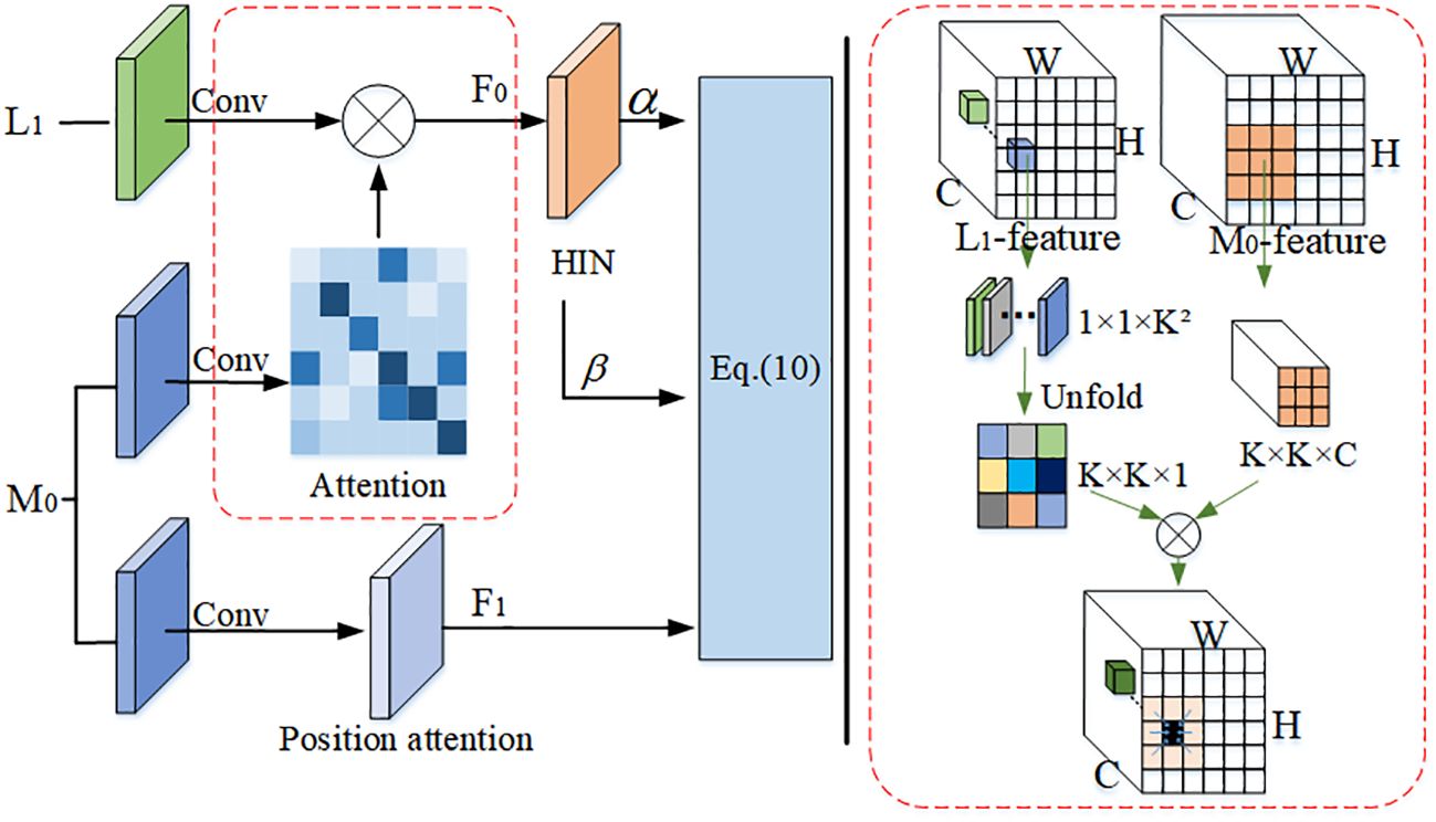
Figure 6 Learnable full-frequency adaptive transformer model.

For the problem of independence of the augmented content of different branches, we calculate the similarity between the L₁ features and the M₀ features to align the augmented content of each branch. Specifically, we first flatten one patch of L₁ ∈ 1 × 1 × K² into a K × K × 1 feature map, then take out the K × K × C size M₀ features centered on the L₁ feature size, and finally multiply the two features and scale them inward as size features. Different patches are processed in turn to obtain each channel and spatial similarity content of the two branches.

For the problem of different sparsity of frequency information, we adopt a half instance normalization (HIN) (Chen et al., 2021) to retain structural information. The normalization method is first applied to the pre-modulation M₀ features and post-modulation F₀ features, then the α and β modulation parameters are obtained by two 3 × 3 convolutions of F₀ features, and finally the F₁ features are modulated as follows (Equation 10):

$\begin{array}{ll}H=\alpha \frac{F_1-\mu }{\delta }+\beta & (10)\end{array}$

where H is the post-processing image features, and µ and δ are means and variances of F₁, respectively.

3.2 Dual discriminator network

Most of the current discriminators of GAN-based underwater image enhancement methods mainly focus on image domain discrimination. However, the difference of image features in the frequency domain is often ignored. To solve this problem, we introduce a dual discriminator to more comprehensively discriminate the authenticity of images.

3.2.1 Discriminator in the image domain

The discriminator requires greater discriminative power for complex training outputs. We have replaced the PatchGAN-style discriminator with a U-Net. The U-Net can obtain more detailed features, but increases the instability of training, and we introduce spectral normalization technology to solve this problem, as shown in Figure 7. With these adjustments, we can achieve better training of the network.

Figure 7

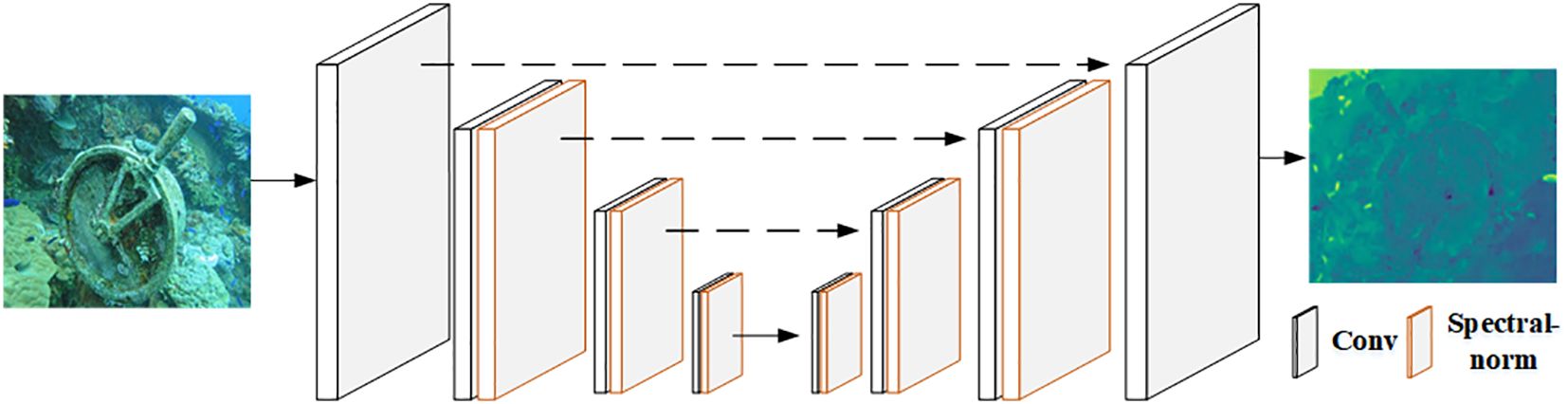
Figure 7 Architecture of the U-Net discriminator with spectral normalization.

3.2.2 Discriminator in the frequency domain

Recent research has shown that there is a gap between the real and generated images in the frequency domain, leading to artifacts in the spatial domain. Based on this observation, we propose the use of a frequency domain discriminator to improve image quality. The ideas in this paper are mainly influenced by the conclusion that a one-dimensional representation of the Fourier power spectrum is sufficient to highlight the differences in the spectra, as proposed by Jung and Keuper (2021). We transform the results of the Fourier transform into polar coordinates and calculate the azimuthal integral.

We propose a spectral discriminator using a full 2D power spectrum and a convolution structure, as in the original discriminator. Firstly, the proposed spectral discriminator takes as input a real or generated image and then calculates the magnitude of its Fourier transform through the spectral transform layer, which converts a 2D image into a 2D array of its spatial frequencies. Next, we calculate the magnitude of the 2D spectrum frequencies and integrate the resulting 2D array for each radius to obtain a one-dimensional profile of the power spectrum. Finally, in order to understand the differences in the higher-frequency bands, we feed the 1D spectral vectors into a high-pass filter and then apply the results to a spectral discriminator. The specific formula is described as follows (Equations 11–13):

$\begin{array}{ll}F(k,l)={\displaystyle {\sum }_{M-1}^{m=0}{\displaystyle {\sum }_{N-1}^{n=0}{e}^{-2\pi i\frac{mk}{M}}{e}^{-2\pi i\frac{nl}{N}}*I(m,n)=F(r,\theta )}}& (11)\end{array}$

$\begin{array}{ll}AI(r)=\frac{1}{2\pi }\underset{2\pi }{\overset{0}{\int }}\left|F(r,\theta )\right|& (12)\end{array}$

$\begin{array}{ll}{F}_{h}p(AI(r))(x)=\{\begin{array}{l}x,r>r_{\tau }\hfill \\ 0,\text{otherwise}\hfill \end{array}& (13)\end{array}$

where F(k, l) denotes calculation of the DFT on two-dimensional image data, in which k ∈ [0, M − 1] and l ∈ [0, N − 1]. AI(r) means the average intensity of the image signal about radial distance r. $F_{h}p$ denotes the high-pass filter. $r_{\tau }$ is a threshold radius for high-pass filtering.

3.3 Loss function

L1 loss (l₁): We use L1 loss on RGB pixels between the predicted J_F and ground-truth images J_T. The formula is as follows (Equation 14):

$\begin{array}{ll}{l}_{l1}={\Vert J_F-J_T\Vert }_1& (14)\end{array}$

Perceptual loss $(l_{perceptual})$: We use perceptual loss (Johnson et al., 2016) to provide additional supervision in the high-level feature space. The formula is as follows (Equation 15):

$\begin{array}{ll}{l}_{Perceptual}={\displaystyle {\sum }_N^{i=1}\Vert Ø(J_F)-Ø(J_T)\Vert }& (15)\end{array}$

where $Ø(·)$ represents the feature maps obtained by the layers within the VGG16 network.

WGAN loss $(l_{WGAN-GP})$: the WGAN-GP loss is adopted and modified into conditional setting as the adversarial loss. The formula is as follows (Equation 16):

$\begin{array}{ll}{l}_{WGAN-GP}=E_{J_F,J_T}[D(J_F,J_T)]-E_{J_F}\left[D(J_F,G(J_F))+\lambda E_{\widehat{J_F}}\left[{(D(\widehat{J_F}))}^2-1\right]\right]& (16)\end{array}$

where J_F and J_T are the original raw image and the ground-truth underwater image, respectively, $\widehat{J_F}$ are the samples along the lines between the generated images G(J_F) and J_T, and λ stands for the weight factor.

GDL loss (l_gdl): We use the GDL function (Fabbri et al., 2018) by directly improving the generator of these predictions by penalizing the image gradient predictions. The formula is as follows (Equation 17):

$\begin{array}{ll}{l}_{gdl}=\sum ^{i,j}{\left|\left|J_{i,j}^T-J_{i-1,j}^T\right|+\left|J_{i,j}^F-J_{i-1,j}^F\right|\right|}^{\alpha }+{\left|\left|J_{i,j}^T-J_{i,j-1}^T\right|+\left|J_{i,j}^F-J_{i,j-1}^F\right|\right|}^{\alpha }& (17)\end{array}$

where J^T means a ground-truth image. J^F stands for predicted image.

The final combination loss is a linear combination of L1 loss, perceptual loss, WGAN loss, and GDL loss (Equation 18):

$\begin{array}{ll}L={\alpha }_1{l}_{l_1}+{\alpha }_2{l}_{\text{WGAN}-\text{GP }}+{\alpha }_3{l}_{\text{perceptual }}+{\alpha }_4{l}_{\text{gdl }}& (18)\end{array}$

where α₁, α₂, α₃, and α₄ are determined through extensive experimental exploration, and we set α₁ = 1, α₂ = 10, α₃ = 2, and α₄ = 10.

4 Experimental results

4.1 Baseline methods

To demonstrate the superiority of our proposed method, we compare 10 advanced underwater image enhancement methods. In more detail, four representative traditional methods are selected for comparison, namely, ULAP (Song et al., 2018), UDCP (Drews et al., 2013), HLRP (Zhuang et al., 2022), and MLLE (Zhang et al., 2022b). Our method is also compared with six deep learning-based methods, namely, USLN (Xiao et al., 2022), URSCT (Ren et al., 2022), UDnet (Saleh et al., 2022), PUIE (Fu et al., 2022b), CWR (Han et al., 2021), and STSC (Wang et al., 2022a). All our experiments are conducted on an NVIDIA Titan RTX GPU (24 GB), 64-GB memory device, and the deep models use the Adam optimizer. The initial learning rate is 1e-2.

4.2 Dataset and evaluation metrics

To train our network, we utilize a dataset comprising 800 labeled images. These images were randomly drawn from the UIEB dataset (Li et al., 2019), which encompasses 890 pairs of underwater images captured across various scenes, exhibiting diverse quality and content. The reference image was selected from among 12 enhanced results by a panel of 50 volunteers.

For assessing our network’s performance, we employ three widely recognized benchmark datasets: UIEB, UCCS (Liu et al., 2020), and UIQS (Liu et al., 2020). Among these, UCCS and UIQS lack reference images, while the UIEB dataset includes them. The UCCS dataset is used primarily for evaluating the efficacy of corrective color models and comprises three subsets, each containing 100 images exhibiting blue, green, and cyan tones, respectively. Meanwhile, the UIQS dataset is chiefly utilized to gauge the correction capabilities of models aimed at enhancing image visibility, featuring a subset with five distinct levels of image quality as measured by UCIQE.

We have used seven commonly used image quality evaluation metrics, namely, peak signal-to-noise ratio (PSNR), structural similarity (SSIM), underwater image quality metric (UIQM) (Panetta et al., 2015), underwater color image quality evaluation (UCIQE) (Yang and Sowmya, 2015), twice mixing (TM) (Fu et al., 2022a), a combination index of colorfulness, contrast, and fog density (CCF) (Wang et al., 2018), and entropy. The UIQM is an image quality evaluation index that comprehensively considers factors such as color, contrast, and clarity of underwater images. The UCIQE is a perceptual model based on color images that takes into account color distortion, contrast changes, and other factors to evaluate the quality of underwater color images by simulating the working mode of the human visual system. The TM evaluates image quality by using two blending ratios in the generation of training data and in the supervised training process. The CCF quantify color loss, blurring, and foggy, respectively. The entropy indicates the entropy value of the image.

4.3 Color restoration on the UCCS dataset

1. Qualitative comparisons: We evaluate the color correction capability of the algorithm on the UCCS dataset with three tones. Figure 8 shows the results of the different methods of processing; here, we focus on the ability of the algorithm to correct the colors. The UDCP method enhances the results with darker colors, where the results for the bluish-green dataset are relatively more realistic. The ULAP method is barely able to process the underwater images and only weakly recovers the results for the bluish dataset. The HLRP method is able to handle underwater images, but still suffers from color bias, and the MLLE method is the best of the traditional image enhancement methods, with some local over-enhancement, such as excessive brightness of stones in the image. The CWR method is a good solution to the problem of underwater color bias, especially in the greenish dataset, but there is an uneven color distribution in the bluish-green dataset. The PUIE method is able to obtain more balanced colors on the bluish-green dataset, but cannot handle the greenish dataset well. The STSC and URSCT methods give greenish and blurred results on both blue-green and greenish datasets. The UDnet method gives bluish results on the UCCS dataset with three tones. The images enhanced by the USLN method appear to be over-processed. Our proposed method gives more balanced and reasonable results in terms of color.

2. Quantitative comparisons: We use five evaluation indicators to further demonstrate the superiority of our approach to color correction. From the metric measures in Table 1, we can draw the following conclusions: (1) It shows that the traditional method enhancement results are not necessarily worse than the deep learning method enhancement processing; for example, the MLLE and HLRP methods show better scores in some metrics. (2) Based on the scores of the UCCS dataset processed by the various methods, the algorithm enhancement results show decreasing scores from the blue data subset to the green data subset. It indicates that the algorithm is able to handle the underwater blue bias problem excellently, but is slightly less capable of solving the green bias problem. (3) The enhanced results of our proposed method are able to obtain essentially optimal scores, and it can be observed that it is difficult to have a method that obtains optimal results on every indicator, probably due to the fact that the various evaluation indicators are biased towards one factor of the image.

Figure 8

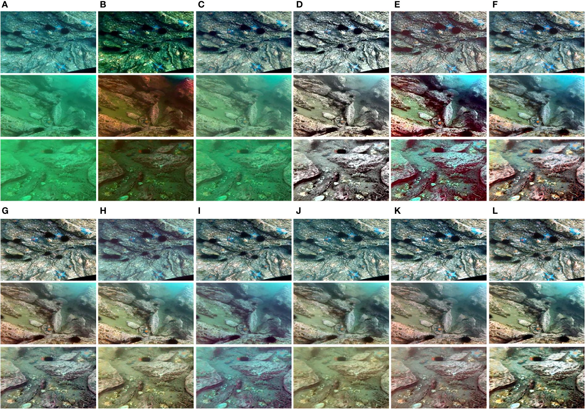
Figure 8 Visualization of the comparative results of the UCCS dataset. The results produced using the following methods: The three inputs are from the blue (first row), blue-green (second row), and green (third row) subsets of the (A) UCCS, (B) UDCP, (C) ULAP, (D) MLLE, (E) HLRP, (F) CWR, (G) PUIE, (H) STSC, (I) UDnet, (J) URSCT, (K) USLN, and (L) OURS data.

Table 1

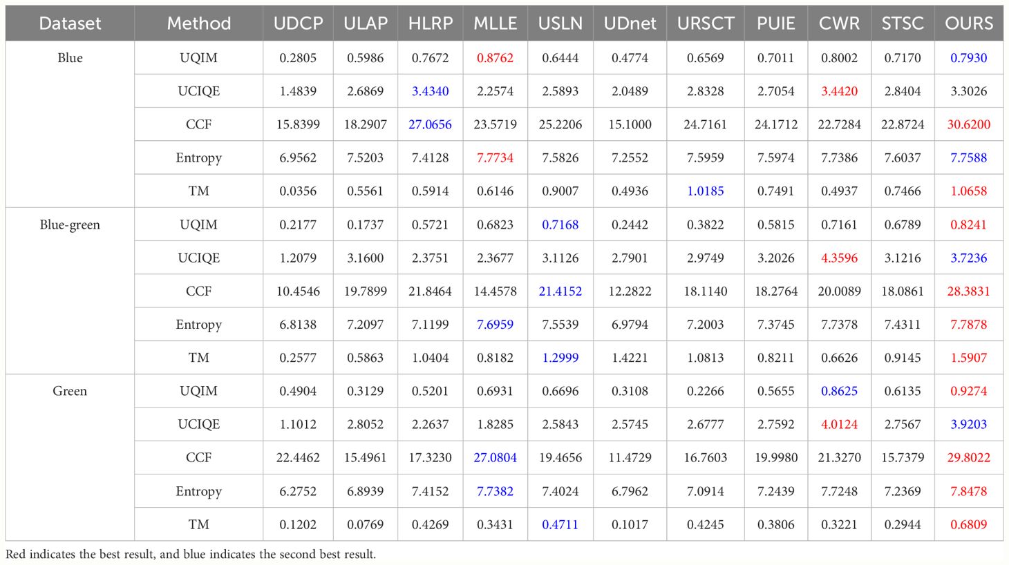
Table 1 Experimental results of different approaches to the UCCS dataset.

4.4 Visibility comparisons on the UIQS dataset

1. Qualitative comparisons: We evaluated the algorithm’s enhanced contrast performance on the UIQS dataset at five levels of different visibility. Figure 9 shows the different algorithm enhancement results. The UDCP and ULAP methods basically fail to enhance the contrast of underwater images, but ULAP gives better results for the A data subset of the UIQS dataset. The MLLE method gives excellent results in images of different contrast levels, but is not ideal for enhancing underwater images with particularly low contrast (subset E). The HLAP method also enhances underwater low contrast to some extent, but not as well as the MLLE method. The results of the STSC and URSCT methods of enhancement are yellowish. The CWR method and the USLN method give the best results for the C subset of images, but the contrast of the enhanced images in the D and E subsets is still low (greenish or bluish). The UDnet method results in low-contrast (bluish) enhancement. The PUIE method is able to solve the low-contrast problem better in the A subset of images, but as the contrast gets lower and lower, the processing becomes less and less effective. Our proposed method gives the best visualization results at all contrast levels.

2. Quantitative comparisons: We use five evaluation indicators to further demonstrate the ability of our method to achieve excellent scores on each level of contrast. From the metric measures in Table 2, we can obtain similar conclusions to those obtained by correcting the color processing results of underwater images.

Figure 9

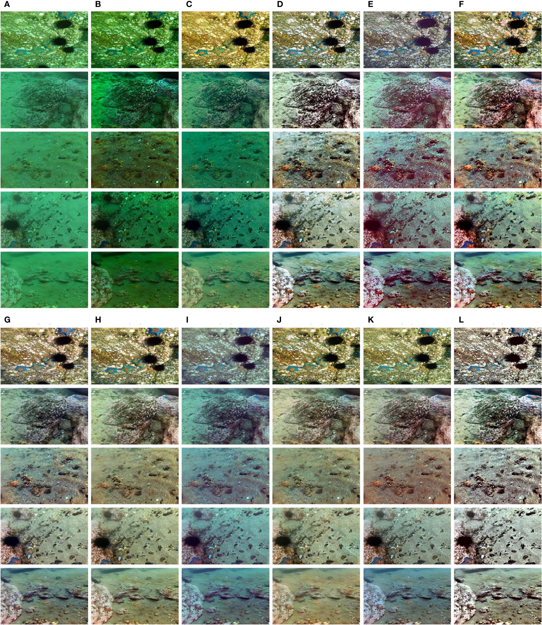
Figure 9 Visualization of the comparison results for the UIQS dataset. Results generated using five inputs from subsets (A) (first row), (B) (second row), (C) (third row), (D) (fourth row), and (E) (fifth row) of the (A) UIQS, (B) UDCP, (C) ULAP, (D) MLLE, (E) HLRP, (F) CWR, (G) PUIE, (H) STSC, (I) UDnet, (J) URSCT, (K) USLN, and (L) OURS data.

Table 2

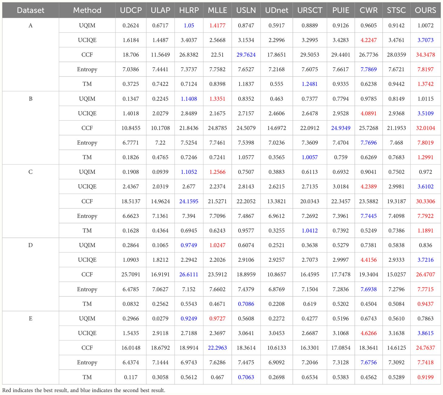
Table 2 Experimental results of different approaches to the UIQS dataset.

Firstly, the traditional method of enhancement was able to obtain images that scored as well as the deep learning enhanced images. Secondly, as the contrast of the underwater images decreases, the scores of the algorithm-enhanced results for each of the image metrics also decrease. Finally, the enhanced results of our proposed method are able to obtain excellent scores in most metrics.

4.5 Comprehensive comparisons on the UIEB dataset

1. Qualitative comparisons: We comprehensively evaluate the superiority of our proposed method on different degraded underwater image datasets (blur, low visibility, low light, color shift, etc.). Figure 10 shows several visual results where the enhanced results of the UDCP and ULAP methods still do not resolve the blue and green bias, and cause color shifts in other colors. The MLLE method over-enhances the results and causes a slight color cast, while the HLAP method is blurrier for border enhancement and does not enhance darker areas as well. The CWR method enhances the color and contrast of underwater images, but with localized brightness overload (first row). The USLN method is able to resolve the underwater color cast, but some images are over-colored (second row). The UDnet method of enhancement results in a blue bias. Both the PUIE and STSC methods solve the problem of underwater color cast, with the STSC method enhancing the high contrast of the results. The URSCT method enhanced the results more satisfactorily. In terms of color and contrast analysis, we can observe that the proposed method enhances the results visually better.

2. Quantitative comparisons: We also quantitatively assessed the ability of these methods to address different degraded data through seven metrics. Table 3 shows the average quantitative scores of the algorithms across the UIEB. Our method has higher PSNR, SSIM, UQIM, UCIQE, CCF, Entropy, and TM values compared to the comparative method. The results show that our method generally produces pleasing visual effects.

Figure 10

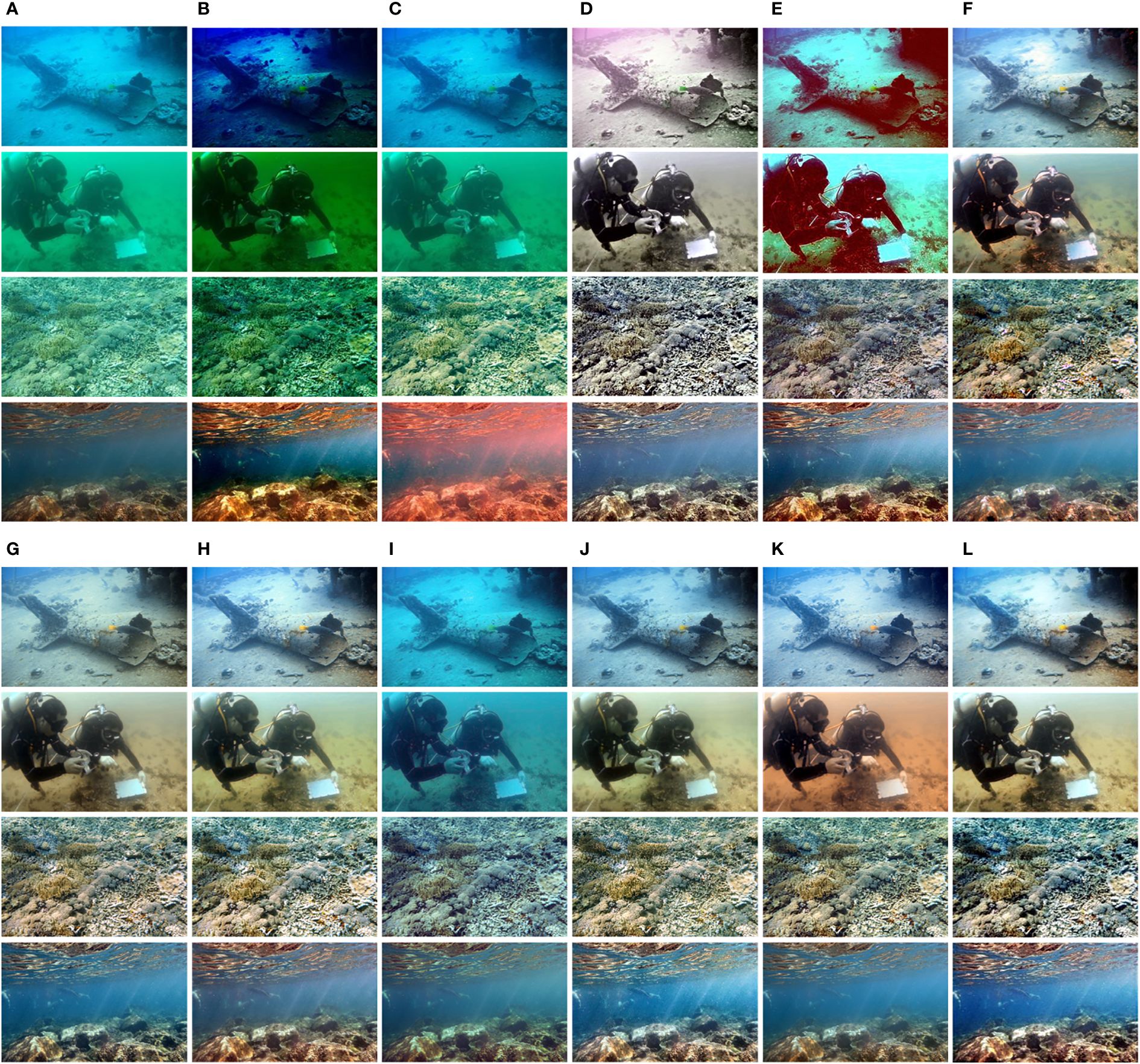
Figure 10 Visualization of the comparison results for the UIEB dataset. Results generated using the inputs of the (A) UIEB, (B) UDCP, (C) ULAP, (D) MLLE, (E) HLRP, (F) CWR, (G) PUIE, (H) STSC, (I) UDnet, (J) URSCT, (K) USLN, and (L) OURS data.

Table 3

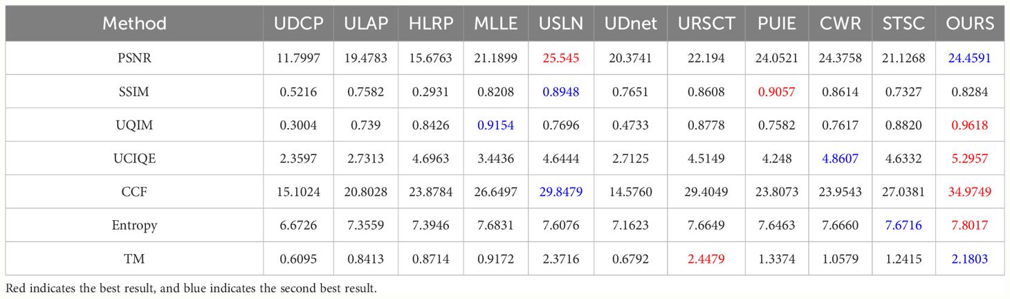
Table 3 Experimental results of different approaches to the UIEB dataset.

4.6 Comparisons of detail enhancement

We observe the superiority of the algorithm by enhancing the local magnification of the image for each algorithm. Figure 11 shows the local features of the images, and it can be seen that the UDCP, ULAP, and UDnet methods enhance the results with color bias and low contrast. The STSC, URSCT, and USLN methods give slightly greenish results; the MLLE and HLRP methods give results as good as the deep learning enhancement; the PUIE method gives low contrast; and the CWR method gives high contrast-enhanced images. The enhanced results of our method give better color and contrast.

Figure 11

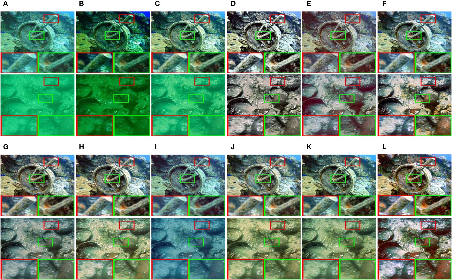
Figure 11 Local visualization comparison results for selected UIEB datasets. Results generated using the inputs of the (A) UIEB, (B) UDCP, (C) ULAP, (D) MLLE, (E) HLRP, (F) CWR, (G) PUIE, (H) STSC, (I) UDnet, (J) URSCT, (K) USLN, and (L) OURS data.

4.7 Structural enhancement comparison

To demonstrate the image structure enhancement effect of our proposed method, the number of visibility edges recovered in the blind contrast enhancement assessment (Hautiere et al., 2008) was measured, as shown in Figure 12. We can observe the following phenomena: (1) The proposed method is able to obtain a higher number of recovered visible edges, confirming its effectiveness in terms of sharpness and contrast enhancement. (2) The enhancement results of the traditional methods are comparable to those of the deep learning methods (HLRP and MLLE methods) and even surpass those of the UDnet method. (3) Our enhancement method, despite being able to obtain the maximum number of visible edges while blurring the target edges (by enhancing many of the background ambient edges as well), may not be beneficial for advanced visual processing.

Figure 12

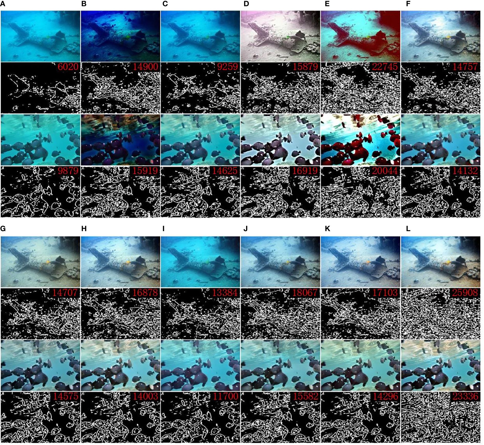
Figure 12 Comparison results for structural enhancement. The red numbers indicate the number of visible edges recovered by the algorithm. The inputs of the (A) UIEB, (B) UDCP, (C) ULAP, (D) MLLE, (E) HLRP, (F) CWR, (G) PUIE, (H) STSC, (I) UDnet, (J) URSCT, (K) USLN, and (L) OURS data.

4.8 Ablation study

We perform ablation experiments on the UCCS, UIQS, and UIEB datasets to illustrate the effectiveness of each component of our approach. The main components include (a) our method without frequency decomposition module (-w/o FD); here, we use the conventional DFT approach as a benchmark; (b) our method without learnable full-frequency transformer module (-w/o LFT); here, we use the regular multi-headed transformer structure as a benchmark; (c) our method without discriminator in the frequency domain (-w/o DFD); and (d) our method with LFT-DGAN.

Figure 13 shows the visualization results for the UCCS, UCIQ, and UIEB datasets. From the visualization results, it can be observed that (1) OURS-w/o FD is able to correct the color of underwater images, but the detail texture is blurred; (2) OURS-w/o LFT is able to recover image texture details but does not work well for color correction and contrast; (3) OURS-w/o DFD can solve the underwater image color and contrast problems well, but the image colors are dark; and (4) our proposed method can further enhance the contrast and color of underwater images.

Figure 13

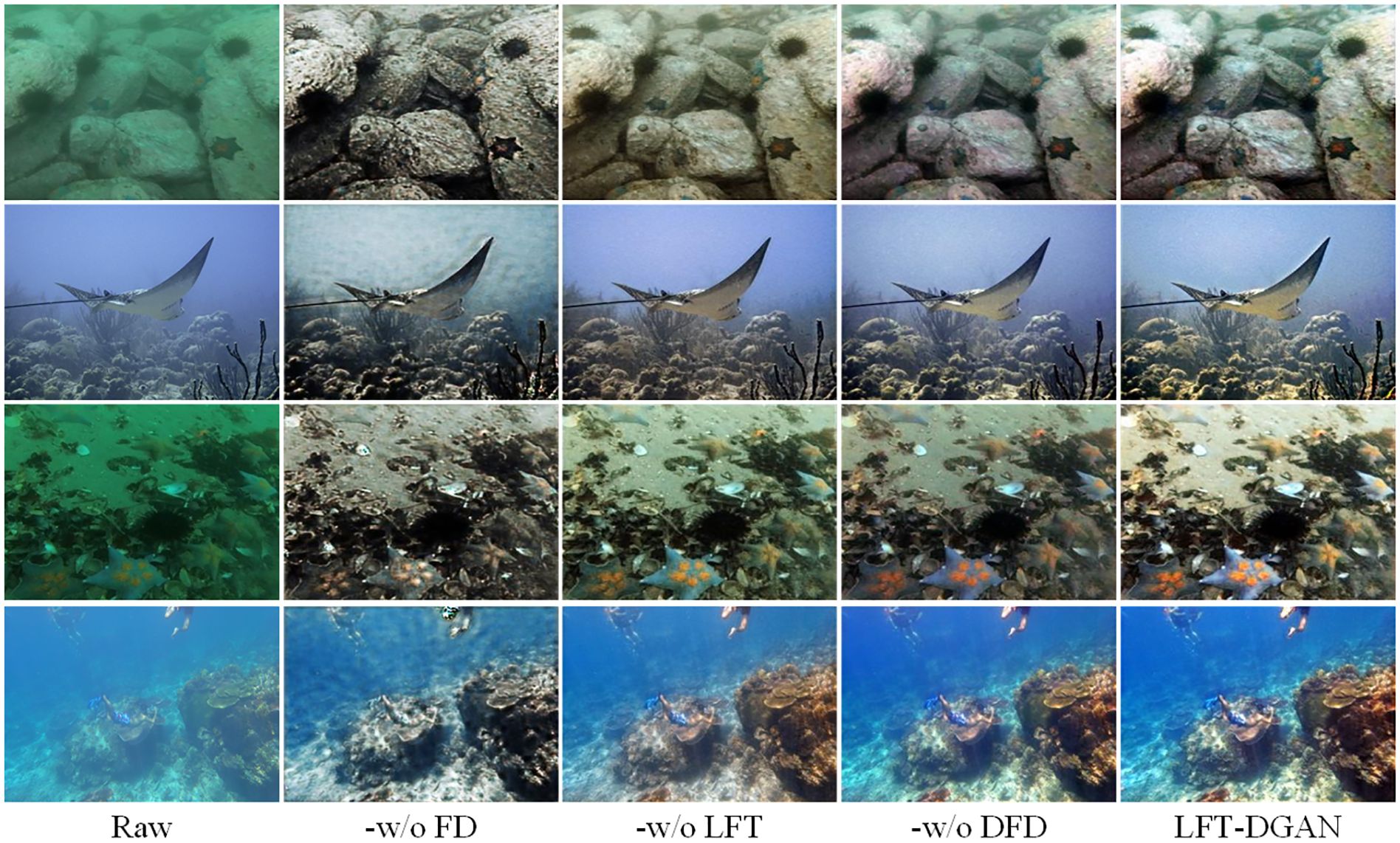
Figure 13 Ablation visualization results for each module in the model in the UCCS, UCIQ, and UIEB datasets.

As shown in Table 4, we quantitatively evaluate the scores for each module of the proposed algorithm, where the UCCS dataset is the average of three subsets and the UIQS dataset is the average of five subsets. It can be seen that each of our proposed modules plays a role in the LFT-DGAN algorithm and that the LFT-DGAN algorithm was able to obtain the best scores.

Table 4

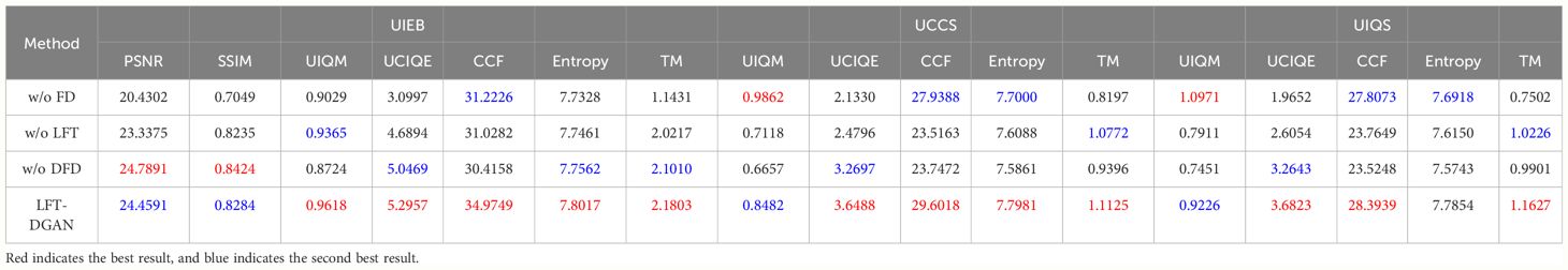
Table 4 Quantitative ablation experiments on the UCCS, UCIQ, and UIEB datasets.

4.9 Generalization performance of our method

We validate the generalization of the LFT-DGAN on different tasks [motion blurring (Rim et al., 2020), brightness (Cai et al., 2018), defogging (Li et al., 2018a), and rain removal (Yasarla and Patel, 2020)]. As can be seen in Figure 14, the LFT-DGAN is able to remove the haze phenomenon better and improve the contrast of the image at different levels of haze images. In the dataset of images with different degrees of motion blur, the LFT-DGAN is only able to remove minor motion blur and does not work well for images with strong motion blur. In images with different degrees of illumination, our method is able to perfectly eliminate the effects of illumination. In images with different levels of rain, the LFT-DGAN is able to resolve the effect of different levels of raindrops on the image and can significantly enhance the image details.

Figure 14

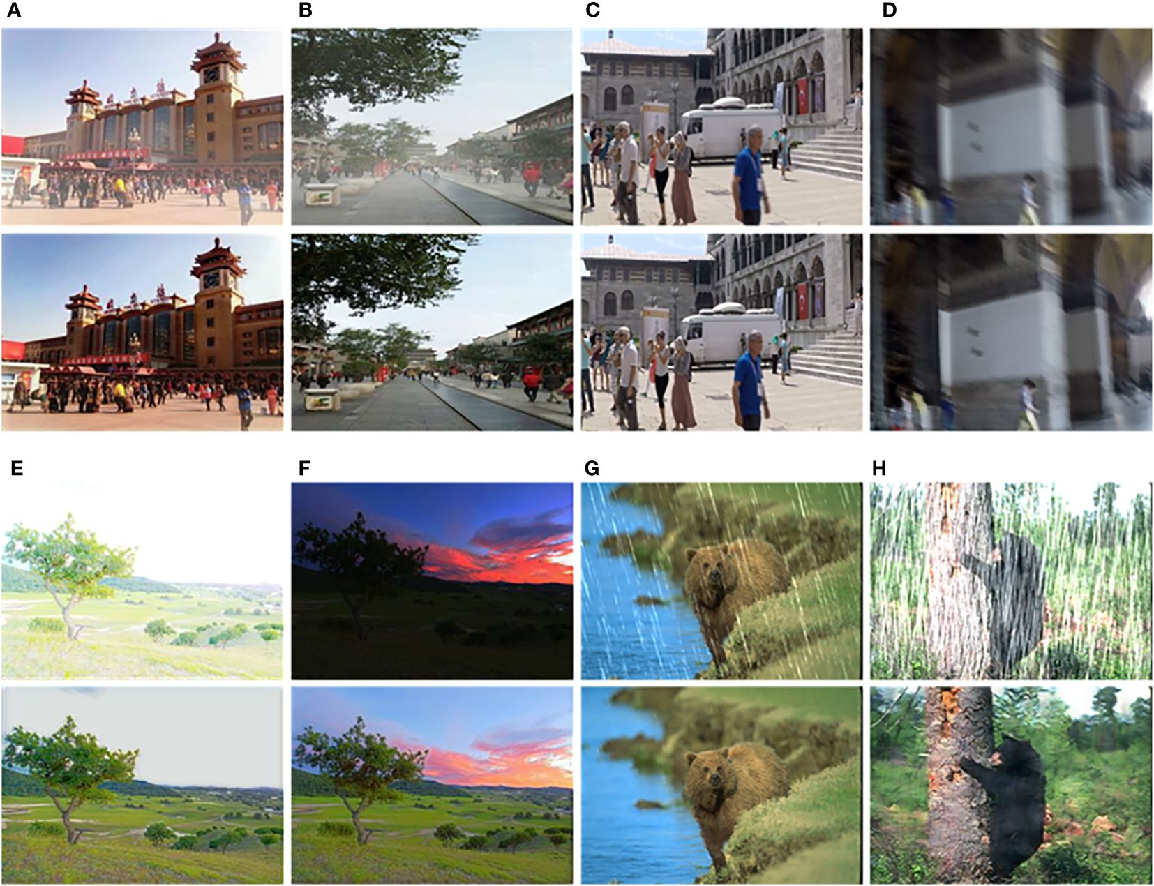
Figure 14 The generalization results of our proposed method (motion blurring, brightness, defogging, and rain removal). (A) Light haze, (B) heavy haze, (C) low motion blurring, (D) high motion blurring, (E) bright light, (F) weak light, (G) light rain, and (H) heavy rain.

5 Conclusion

In this paper, an underwater single-image enhancement method that can learn from an LFT-DGAN is proposed. Experimental results show that the advantages of the proposed method are summarized as follows: (1) A new image frequency domain decomposition method is designed using reversible convolutional networks, which can effectively separate low-, medium-, and high-frequency image information from underwater images. Note that the frequency domain decomposition method in this paper can be applied not only in the field of image enhancement, but also in other fields. (2) We have designed a custom transformer for frequency domain image feature enhancement that takes full account of underwater image space and channel correlation to effectively address underwater image color and contrast issues. (3) We design a dual discriminator method in the spatial and frequency domains, taking into account the differences between spatial and frequency domain underwater image features in order to reduce the differences between images. (4) The proposed model is able to operate directly at the pixel level without additional conditional priors. (5) The combined analysis shows that our proposed method performs superiorly on multiple datasets. Moreover, the ablation experiments also demonstrate the effectiveness of each module.

Although our method has good performance, it also has some limitations. The image enhancement method proposed in this paper is able to achieve pleasing results, but whether it is beneficial to the high-level domain deserves further investigation. In addition, current underwater imagery consists mainly of sonar imaging (Zhang et al., 2021b; Zhang, 2023) and optical camera imaging. Since sonar imaging uses acoustic signals while camera imaging uses optical signals, there are significant differences between the two methods. It is difficult for the method in this paper to perform mutual transfer learning. In future work, we intend to address the above issues.

Data availability statement

The original contributions presented in the study are included in the article/supplementary material. Further inquiries can be directed to the corresponding authors.

Author contributions

SJZ: Methodology, Writing – original draft. RW: Supervision, Funding acquisition, Writing – review & editing. STZ: Conceptualization, Data curation, Writing – review & editing. LW: Formal Analysis, Visualization, Writing – review & editing. ZL: Supervision, Writing – review & editing.

Funding

The author(s) declare financial support was received for the research, authorship, and/or publication of this article. This work was supported by the National Key R&D Program of China (2019YFE0125700) and the National Natural Science Foundation of China (Grant No. 31671586).

Conflict of interest

The authors declare that the research was conducted in the absence of any commercial or financial relationships that could be construed as a potential conflict of interest.

Publisher’s note

All claims expressed in this article are solely those of the authors and do not necessarily represent those of their affiliated organizations, or those of the publisher, the editors and the reviewers. Any product that may be evaluated in this article, or claim that may be made by its manufacturer, is not guaranteed or endorsed by the publisher.

References

Cai J., Gu S., Zhang L. (2018). Learning a deep single image contrast enhancer from multi-exposure images. IEEE Trans. Image Process. 27, 2049–2062. doi: 10.1109/TIP.2018.2794218

CrossRef Full Text | Google Scholar

Chen Y., Fan H., Xu B., Yan Z., Kalantidis Y., Rohrbach M., et al. (2019). “Drop an octave: Reducing spatial redundancy in convolutional neural networks with octave convolution,” in Proceedings of the IEEE/CVF international conference on computer vision. (New York, USA: IEEE), 3435–3444.

Google Scholar

Chen L., Lu X., Zhang J., Chu X., Chen C. (2021). “Hinet: Half instance normalization network for image restoration,” in Proceedings of the IEEE/CVF Conference on Computer Vision and Pattern Recognition. (New York, USA: IEEE), 182–192.

Google Scholar

Dinh L., Krueger D., Bengio Y. (2014). Nice: Non-linear independent components estimation. arXiv preprint arXiv:1410.8516.

Google Scholar

Drews P., Nascimento E., Moraes F., Botelho S., Campos M. (2013). “Transmission estimation in underwater single images,” in Proceedings of the IEEE international conference on computer vision workshops. (New York, USA: IEEE), 825–830.

Google Scholar

Fabbri C., Islam M. J., Sattar J. (2018). “Enhancing underwater imagery using generative adversarial networks,” in 2018 IEEE International Conference on Robotics and Automation (ICRA). (New York, USA: IEEE), 7159–7165.

Google Scholar

Fu Z., Fu X., Huang Y., Ding X. (2022a). Twice mixing: a rank learning based quality assessment approach for underwater image enhancement. Signal Processing: Image Communication 102, 116622.

Google Scholar

Fu Z., Wang W., Huang Y., Ding X., Ma K.-K. (2022b). “Uncertainty inspired underwater image enhancement,” in Computer Vision–ECCV 2022: 17th European Conference. (Tel Aviv, Israel: IEEE), October 23–27, 2022. 465–482.

Google Scholar

Ghani A. S. A., Isa N. A. M. (2017). Automatic system for improving underwater image contrast and color through recursive adaptive histogram modification. Comput. Electron. Agric. 141, 181–195. doi: 10.1016/j.compag.2017.07.021

CrossRef Full Text | Google Scholar

Guan Z., Jing J., Deng X., Xu M., Jiang L., Zhang Z., et al. (2022). Deepmih: Deep invertible network for multiple image hiding. IEEE Trans. Pattern Anal. Mach. Intell. 45, 372–390. doi: 10.1109/TPAMI.2022.3141725

PubMed Abstract | CrossRef Full Text | Google Scholar

Han J., Shoeiby M., Malthus T., Botha E., Anstee J., Anwar S., et al. (2021). “Single underwater image restoration by contrastive learning,” in 2021 IEEE International Geoscience and Remote Sensing Symposium IGARSS. (New York, USA: IEEE), 2385–2388.

Google Scholar

Hautiere N., Tarel J.-P., Aubert D., Dumont E. (2008). Blind contrast enhancement assessment by gradient ratioing at visible edges. Image Anal. Stereology 27, 87–95. doi: 10.5566/ias.v27.p87-95

CrossRef Full Text | Google Scholar

Jiang B., Li J., Li H., Li R., Zhang D., Lu G. (2023). Enhanced frequency fusion network with dynamic hash attention for image denoising. Inf. Fusion 92, 420–434. doi: 10.1016/j.inffus.2022.12.015

CrossRef Full Text | Google Scholar

Johnson J., Alahi A., Fei-Fei L. (2016). “Perceptual losses for real-time style transfer and super-resolution,” in Computer Vision–ECCV 2016: 14th European Conference. (Amsterdam, The Netherlands: IEEE), October 11–14, 2016. 694–711.

Google Scholar

Jung S., Keuper M. (2021). “Spectral distribution aware image generation,” in Proceedings of the AAAI conference on artificial intelligence (British Columbia, Canada: AAAI), 35. 1734–1742.

Google Scholar

Kang Y., Jiang Q., Li C., Ren W., Liu H., Wang P. (2022). A perception-aware decomposition and fusion framework for underwater image enhancement. IEEE Trans. Circuits Syst. Video Technol.

Google Scholar

Kingma D. P., Dhariwal P. (2018). Glow: Generative flow with invertible 1x1 convolutions. Adv. Neural Inf. Process. Syst. 31.

Google Scholar

Li F., Di X., Zhao C., Zheng Y., Wu S. (2022). Fa-gan: a feature attention gan with fusion discriminator for non-homogeneous dehazing. Signal Image Video Process. 16(5), 1243–1251. doi: 10.1007/s11760-021-02075-1

CrossRef Full Text | Google Scholar

Li C., Guo J., Guo C. (2018b). Emerging from water: Underwater image color correction based on weakly supervised color transfer. IEEE Signal Process. Lett. 25, 323–327. doi: 10.1109/LSP.2018.2792050

CrossRef Full Text | Google Scholar

Li C., Guo C., Ren W., Cong R., Hou J., Kwong S., et al. (2019). An underwater image enhancement benchmark dataset and beyond. IEEE Trans. Image Process. 29, 4376–4389. doi: 10.1109/TIP.83

CrossRef Full Text | Google Scholar

Li X., Jin X., Yu T., Sun S., Pang Y., Zhang Z., et al. (2021). Learning omni-frequency region-adaptive representations for real image super-resolution. Proc. AAAI Conf. Artif. Intell. 35, 1975–1983. doi: 10.1609/aaai.v35i3.16293

CrossRef Full Text | Google Scholar

Li B., Ren W., Fu D., Tao D., Feng D., Zeng W., et al. (2018a). Benchmarking single-image dehazing and beyond. IEEE Trans. Image Process. 28, 492–505. doi: 10.1109/TIP.83

CrossRef Full Text | Google Scholar

Liu R., Fan X., Zhu M., Hou M., Luo Z. (2020). Real-world underwater enhancement: Challenges, benchmarks, and solutions under natural light. IEEE Trans. Circuits Syst. Video Technol. 30, 4861–4875. doi: 10.1109/TCSVT.76

CrossRef Full Text | Google Scholar

Liu Y., Qin Z., Anwar S., Ji P., Kim D., Caldwell S., et al. (2021). “Invertible denoising network: A light solution for real noise removal,” in Proceedings of the IEEE/CVF conference on computer vision and pattern recognition. (New York, USA: IEEE), 13365–13374.

Google Scholar

Ma Z., Oh C. (2022). “A wavelet-based dual-stream network for underwater image enhancement,” in ICASSP 2022–2022 IEEE International Conference on Acoustics, Speech and Signal Processing (ICASSP). (New York, USA: IEEE), 2769–2773.

Google Scholar

Panetta K., Gao C., Agaian S. (2015). Human-visual-system-inspired underwater image quality measures. IEEE J. Oceanic Eng. 41, 541–551. doi: 10.1109/JOE.2015.2469915

CrossRef Full Text | Google Scholar

Ren T., Xu H., Jiang G., Yu M., Zhang X., Wang B., et al. (2022). Reinforced swin-convs transformer for simultaneous underwater sensing scene image enhancement and super-resolution. IEEE Trans. Geosci. Remote Sens. 60, 1–16. doi: 10.1109/TGRS.2022.3205061

CrossRef Full Text | Google Scholar

Rim J., Lee H., Won J., Cho S. (2020). “Real-world blur dataset for learning and benchmarking deblurring algorithms,” in Computer Vision–ECCV 2020: 16th European Conference, (Glasgow, UK: IEEE), August 23–28, 2020. 184–201.

Google Scholar

Saleh A., Sheaves M., Jerry D., Azghadi M. R. (2022). Adaptive uncertainty distribution in deep learning for unsupervised underwater image enhancement. arXiv preprint arXiv:2212.08983.

Google Scholar

Song W., Wang Y., Huang D., Tjondronegoro D. (2018). “A rapid scene depth estimation model based on underwater light attenuation prior for underwater image restoration,” in Advances in Multimedia Information Processing–PCM 2018: 19th Pacific-Rim Conference on Multimedia. (Hefei, China: Springer), September 21–22, 2018. 678–688.

Google Scholar

Wang N., Chen T., Kong X., Chen Y., Wang R., Gong Y., et al. (2023a). Underwater attentional generative adversarial networks for image enhancement. IEEE Trans. Human-Machine Syst. doi: 10.1109/THMS.2023.3261341

CrossRef Full Text | Google Scholar

Wang N., Chen T., Liu S., Wang R., Karimi H. R., Lin Y. (2023b). Deep learning-based visual detection of marine organisms: A survey. Neurocomputing 532, 1–32. doi: 10.1016/j.neucom.2023.02.018

CrossRef Full Text | Google Scholar

Wang Y., Guo J., Gao H., Yue H. (2021). Uiecˆ 2-net: Cnn-based underwater image enhancement using two color space. Signal Processing: Image Communication 96, 116250.

Google Scholar

Wang Y., Li N., Li Z., Gu Z., Zheng H., Zheng B., et al. (2018). An imaging-inspired no-reference underwater color image quality assessment metric. Comput. Electrical Eng. 70, 904–913. doi: 10.1016/j.compeleceng.2017.12.006

CrossRef Full Text | Google Scholar

Wang D., Ma L., Liu R., Fan X. (2022a). “Semantic-aware texture-structure feature collaboration for underwater image enhancement,” in 2022 International Conference on Robotics and Automation (ICRA). (New York, USA: IEEE), 4592–4598. doi: 10.1109/ICRA46639.2022.9812457

CrossRef Full Text | Google Scholar

Wang L., Xu L., Tian W., Zhang Y., Feng H., Chen Z. (2022b). Underwater image super-resolution and enhancement via progressive frequency-interleaved network. J. Visual Communication Image Representation 86, 103545. doi: 10.1016/j.jvcir.2022.103545

CrossRef Full Text | Google Scholar

Wu S., Luo T., Jiang G., Yu M., Xu H., Zhu Z., et al. (2021). A two-stage underwater enhancement network based on structure decomposition and characteristics of underwater imaging. IEEE J. Oceanic Eng. 46, 1213–1227. doi: 10.1109/JOE.2021.3064093

CrossRef Full Text | Google Scholar

Xiao Z., Han Y., Rahardja S., Ma Y. (2022). Usln: A statistically guided lightweight network for underwater image enhancement via dual-statistic white balance and multi-color space stretch. arXiv preprint arXiv:2209.02221.

Google Scholar

Xiao M., Zheng S., Liu C., Wang Y., He D., Ke G., et al. (2020). “Invertible image rescaling,” in Computer Vision–ECCV 2020: 16th European Conference (Glasgow, UK: IEEE), August 23–28, 2020. 126–144.

Google Scholar

Yang M., Sowmya A. (2015). An underwater color image quality evaluation metric. IEEE Trans. Image Process. 24, 6062–6071. doi: 10.1109/TIP.2015.2491020

PubMed Abstract | CrossRef Full Text | Google Scholar

Yasarla R., Patel V. M. (2020). Confidence measure guided single image de-raining. IEEE Trans. Image Process. 29, 4544–4555. doi: 10.1109/TIP.83

CrossRef Full Text | Google Scholar

Zhang X. (2023). An efficient method for the simulation of multireceiver sas raw signal. Multimedia Tools Appl., 1–18. doi: 10.1007/s11042-023-16992-5

CrossRef Full Text | Google Scholar

Zhang W., Dong L., Xu W. (2022a). Retinex-inspired color correction and detail preserved fusion for underwater image enhancement. Comput. Electron. Agric. 192, 106585. doi: 10.1016/j.compag.2021.106585

CrossRef Full Text | Google Scholar

Zhang W., Dong L., Zhang T., Xu W. (2021a). Enhancing underwater image via color correction and bi-interval contrast enhancement. Signal Processing: Image Communication 90, 116030. doi: 10.1016/j.image.2020.116030

CrossRef Full Text | Google Scholar

Zhang X., Wu H., Sun H., Ying W. (2021b). Multireceiver sas imagery based on monostatic conversion. IEEE J. Selected Topics Appl. Earth Observations Remote Sens. 14, 10835–10853. doi: 10.1109/JSTARS.2021.3121405

CrossRef Full Text | Google Scholar

Zhang W., Zhuang P., Sun H.-H., Li G., Kwong S., Li C. (2022b). Underwater image enhancement via minimal color loss and locally adaptive contrast enhancement. IEEE Trans. Image Process. 31, 3997–4010. doi: 10.1109/TIP.2022.3177129

CrossRef Full Text | Google Scholar

Zheng S., Wang R., Zheng S., Wang F., Wang L., Liu Z. (2023). A multi-scale feature modulation network for efficient underwater image enhancement. J. King Saud University-Computer Inf. Sci. 36 (1), 101888. doi: 10.1016/j.jksuci.2023.101888

CrossRef Full Text | Google Scholar

Zhuang P., Wu J., Porikli F., Li C. (2022). Underwater image enhancement with hyper-laplacian reflectance priors. IEEE Trans. Image Process. 31, 5442–5455. doi: 10.1109/TIP.2022.3196546

PubMed Abstract | CrossRef Full Text | Google Scholar

Appendix

Power spectral density image

To analyze the influence of the image frequency domain distribution, we rely on the Fourier power spectrum with a one-dimensional representation of the features. First, we calculate the spectral representation from the DFT of a two-dimensional image of size M*N. The specific formula is (Equation A1):

$\begin{array}{ll}P(u,v)=|\sum _{m=0}^{N-1}\sum _{n=0}^{N-1}f(m,n)·e^{-i2\pi (\frac{mu}{N}+\frac{nv}{N}){|}^2}& \text{(A1)}\end{array}$

In this equation, P(u,v) represents the power spectrum of the image, while f(m,n) represents the pixel values of the original image in the spatial domain. The symbol Σ denotes summation, indicating that we sum over all values of m and n. The symbol i represents the imaginary unit, while u and v respectively denote the coordinates in the frequency domain, and m and n represent the coordinates in the spatial domain. N represents the size or dimensions of the image. Secondly, by integrating the azimuth angle at the radial frequency, the one-dimensional power spectral density of the image at the radial frequency θ can be obtained. The specific formula is (Equation A2):

$\begin{array}{ll}AI(r)=\frac{1}{2\pi }\underset{2\pi }{\overset{0}{\int }}|P(u,v)(r,\theta )|& \text{(A2)}\end{array}$

Param, flops, memory, and running time comparisons

In order to fully detect the efficiency of our proposed method, we based on the number of parameters (#Pama), number of floating point operations per second (#Flops), GPU memory consumption (#GPU Mem.) and running time (#Avg.Time). Among them, #Flops is the calculation value of the underwater image whose input size is 256*256. #Avg.Time is the average time for testing 100 underwater images with a size of 620*460. The results are shown in Table A1. Our proposed method can basically maintain a smaller footprint in terms of parameter volume and running floating point numbers, but our proposed method can achieve the optimal image enhancement results, secondly, in terms of memory footprint and average test running time. It can also achieve more excellent results.

Table A1

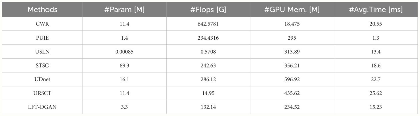
Table A1 Comparison of parameter counts, floating-point operation per second, memory, and runtime.