Modelling mass accumulation rates and 210Pb rain rates in the Skagerrak: lateral sediment transport dominates the sediment input

1 Introduction

Bulk sediment fluxes control the transport and distribution of many substances in the water and sediment column, such as organic carbon and pollutants. Furthermore, in coastal and shelf regions that are used economically, sediment budgets are crucial to assess the anthropogenic pressure on the natural systems, such as the disturbance of surface sediments and redistribution of sedimentary material, and to set up management plans for seafloor resources (Walling and Collins, 2008; Morang et al., 2012). An integral part of the sediment cycle is the accumulation and subsequent burial of particles at the seafloor, which acts as the ultimate sink in many marine geochemical mass balances. In regional sediment budgets, estimates of area-wide sediment mass accumulation rates (MAR) are often obtained by averaging and subsequent upscaling of the average MAR to the study area extent. This approach has been applied in previous studies to estimate sediment budgets in the North Sea and Skagerrak (van Weering et al., 1987; Bøe et al., 1996; de Haas et al., 1996; de Haas and van Weering, 1997). However, the traditional upscaling technique is unable to resolve non-linear spatial heterogeneities between individual data sites, which is particularly important in such dynamic regions. As a result, current area-wide quantifications derived using the averaging technique are likely associated with high uncertainties.

The Skagerrak represents the largest depocenter for sediments from the North Sea. With the dynamic hydrography, complex seabed topography and high data density, the Skagerrak offers an ideal setting to examine MAR in an environment with various sedimentation patterns. Furthermore, the Skagerrak and North Sea sedimentary systems have been increasingly impacted by anthropogenic activities such as bottom trawling (ICES, 2020), sediment extraction (De Groot, 1986; ICES, 2019; Mielck et al., 2019) or offshore wind park constructions (Heinatz and Scheffold, 2023) since industrial times. Hence, sediment budgeting in this area may improve our understanding of sediment redistribution in a changing environment. In this study, a machine learning approach was applied to upscale the gathered data from literature studies and own sampling campaigns and predict the spatial distributions of sediment water content (porosity) and ²¹⁰Pb rain rates in the Skagerrak. Based on the modeled porosity and published spatial data on sedimentation rates (Diesing et al., 2021), we present an area-wide MAR and compare it to previous estimates. The radionuclide ²¹⁰Pb is known to be readily scavenged by particles in the water column and to settle alongside sediments (e.g. Krishnaswamy et al., 1971; Nittrouer et al., 1979; Nozaki et al., 1991). Hence, the spatial distribution of ²¹⁰Pb rain rates serves as an indicator of sedimentation rates and is compared to the sedimentation patterns previously presented in Diesing et al. (2021). Furthermore, area-wide ²¹⁰Pb rain rates are utilized to estimate the contributions of local and lateral inputs in the Skagerrak. Finally, we compare the machine learning approach with previous estimates based on upscaling that used the averaging approach.

2 Study area

The Skagerrak is located between Denmark, Norway, and Sweden and connects the North Sea and the Kattegat, with water depths reaching about 700 meters (Figure 1). The Jutland current carries water and suspended particles from the central and southern North Sea to the Skagerrak, where it meets the Baltic current and continues to circulate anticlockwise before leaving the Skagerrak northward through the Norwegian Coastal Current (van Weering et al., 1987; Otto et al., 1990). Towards the northeastern Skagerrak, current velocities decrease and the particles transported into the Skagerrak settle. As a result, the Skagerrak sediments are characterized by a large lateral input primarily consisting of lithogenic material from the North Sea (van Weering et al., 1993; de Haas and van Weering, 1997). The sediment composition varies throughout the region, with sand (< 40% clay) being common along the Danish coast while fine-grained silt and clay sediments dominate the Skagerrak basin at water depth below ~150 m (Stevens et al., 1996; Mitchell et al., 2019a). The sediment column is potentially subject to substantial reworking due to bottom trawling by fisheries at water depths shallower than approximately 300-500 m (ICES, 2020).

Figure 1

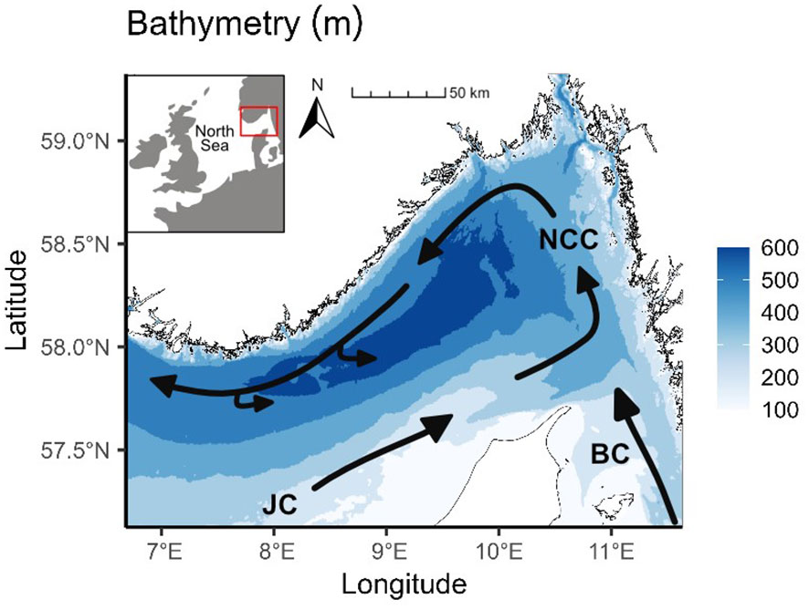
Figure 1 Study area with information on water depth. Black arrows indicate the current regime. The Jutland Current (JC) originates from the south and merges with the Baltic Current (BC) to form the Norwegian Coastal Current (NCC), which leaves the Skagerrak northwards.

3 Materials and methods

A machine learning model was employed to scale up the data of individual stations and determine the spatial distributions of the desired variables porosity and ²¹⁰Pb rain rate (response variables). In principle, high-resolution spatial data of parameters that were assumed to correlate with the response variables, e.g. bathymetry or grain size (predictor variables), were sourced from the available literature in the study area. These predictor variables were leveraged by the model to predict the spatial distribution of the response variables at the same resolution as the predictors using a quantile regression forest (QRF) algorithm (Meinshausen, 2006).

3.1 Data collection

3.1.1 Response variables

Most of the data used to determine the spatial distribution of porosity were sourced from the PANGAEA database by applying a data warehouse search over the area of interest. The downloaded data were filtered to retain records with realistic porosity values between 20% and 100%, as the range of typical values of porosity is 50 - 90% for unconsolidated muddy sediments and 25 - 50% for sandy sediments (Richardson and Jackson, 2017). Additionally, we limited the dataset to the upper 0.1 m of sediment depth. Data on ²¹⁰Pb were collected from various publications (Erlenkeuser and Pederstad, 1984; Erlenkeuser, 1985; van Weering et al., 1987; Wilken et al., 1990; van Weering et al., 1993; Paetzel et al., 1994; Beks, 2000; Ståhl et al., 2004; Ferdelman, 2005a, b, c; Deng et al., 2020). A full summary of the porosity and ²¹⁰Pb data is given in the supplement (Tables S1, S2). The literature data were complemented with data from nine short sediment cores (< 50 cm) recovered over two sampling campaigns in the Skagerrak, AL557 and AL561, with R/V Alkor in June and August 2021, respectively (Schmidt, 2021; Thomas et al., 2022; Spiegel et al., 2023). Porosity was determined by weighting sediment samples before and after conventional drying in an oven or freeze-drying. The porosity was then calculated from the difference between the two weights and the density of dry solids of the sediment, which was either measured or assumed (2.3 - 2.6 g cm^-3). Measurements of ²¹⁰Pb were carried out by alpha or gamma spectrometry. In marine sediments, the term excess ²¹⁰Pb (²¹⁰Pb_ex) refers to the ²¹⁰Pb content that is introduced by sinking particles and excludes the ²¹⁰Pb resulting from the natural background decay of ²²⁶Ra within the sediment column. ²¹⁰Pb_ex values were obtained either by subtracting the natural background activities of ²²⁶Ra or by subtracting the steady-state ²¹⁰Pb activity in sediment depths below the profile of exponential ²¹⁰Pb decay. In some studies, the raw ²¹⁰Pb values were not explicitly provided but were depicted either as linear or double logarithmic plots. In those cases, the activity data were carefully extracted from the figures by graphical evaluation. In total, the dataset consists of porosity and ²¹⁰Pb data gathered from 194 and 65 locations, respectively (Figure 2; Tables S1, S2). Averaging porosity values in the same grid cell of the model resulted in 145 porosity values for the machine learning procedure (see section 3.2).

Figure 2

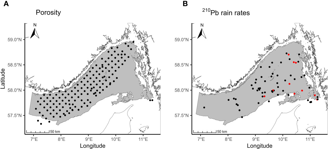
Figure 2 Stations where data was available for (A) porosity and (B) ²¹⁰Pb rain rates that were utilized for spatial predictions. The gray area refers to the area of applicability (AOA) of the model. Stations marked in red indicate disturbed ²¹⁰Pb profiles that do not reach natural background levels at the bottom of the sediment core, likely due to physical mixing by currents and waves or bottom trawling.

To determine total ²¹⁰Pb rain rates to the seafloor (FPb), the ²¹⁰Pb_ex activity data were integrated over the sediment column ranging from the surface (0) to the depth where the ²¹⁰Pb activities reached natural background levels (max) and multiplied by the decay constant (Cochran et al., 1990; Alperin et al., 2002):

$\begin{array}{ll}\text{FPb}=\underset{0}{\overset{\text{max}}{\int }}\text{Pb}·\text{λ}·{\text{ρ}}_{\text{DB}}\text{ dx}& (1)\end{array}$

$\begin{array}{ll}{\text{ρ}}_{\text{DB}}=\text{ds}·(1-\mathrm{\varphi })& (2)\end{array}$

where Pb is the ²¹⁰Pb_ex activity, λ is the ²¹⁰Pb decay constant (0.031 yr^-1), ρ_DB is the dry bulk density, ds is the density of dry solids that was assumed to be 2.5 g cm^-3 and ϕ is depth-dependent porosity. An interpolation function was fitted through the downcore ²¹⁰Pb_ex data using the program Mathematica 12.2. This function was integrated over the entire sediment core to determine the depth-integrated ²¹⁰Pb_ex activity. At 10 stations, ²¹⁰Pb_ex at the bottom of the sediment core did not reach natural background levels. Hence, the ²¹⁰Pb_ex inventories were underestimated at these sites to an uncertain extent (highlighted in red in Figure 2B). Considering the exponential decline of ²¹⁰Pb_ex activities with sediment depth, and generally low ²¹⁰Pb_ex activities observed at these sites, a relatively minor error was expected by including these stations.

For a comparison between atmospheric ²¹⁰Pb input rates and total ²¹⁰Pb rain rates, it is usually necessary to consider the production of ²¹⁰Pb by the in-situ decay of ²²⁶Ra in the water column (Cochran et al., 1990). However, given the long half-life of ²²⁶Ra (1600 yr), along with the large sedimentary inventory of ²¹⁰Pb and relatively shallow water depths in the Skagerrak, the decay of ²²⁶Ra in the water column contributes< 1% to the sedimentary ²¹⁰Pb pool. Thus, a correction for this fraction was not performed.

3.1.2 Predictor variables

Initially, a wide range of potential predictor variables was selected considering their data availability at a sufficient spatial resolution and full area coverage in the Skagerrak, including topographic, sedimentological, hydrodynamic, and oceanographic variables. Porosity and ²¹⁰Pb rain rates were expected to be controlled by particle transport and the characteristics of the transported particles in the Skagerrak. Hence, bathymetry, current velocity, distance to the shoreline and suspended particulate matter concentrations were chosen as predictor variables as they directly or indirectly reflect particle transport and distribution (Table 1). Since the particle size has been shown to be closely related to porosity (Wilson et al., 2018), the content of silt and clay in surface sediments was also chosen as a predictor variable. Furthermore, the ratio of the tidal benthic boundary layer thickness to water depth is important for sediment transport dynamics near the seabed (Williams et al., 2019) and was deemed an important environmental control on sediment fluxes in a previous study (Diesing et al., 2021). Temperature and salinity were also included as predictor variables as they have been shown to reflect the contributions of different water masses to the Skagerrak, i.e. from the North Sea, Baltic Sea and local riverine input (Kristiansen and Aas, 2015) that carry the sediment and ²¹⁰Pb into the Skagerrak. Despite ²¹⁰Pb being closely related to bulk sediment fluxes, we opted to exclude the spatial distribution of sedimentation rates (Diesing et al., 2021) from the list of predictor variables. This decision was made to avoid circularity arguments, as the presented sedimentation rate data in the literature itself is derived from ²¹⁰Pb measurements.

Table 1

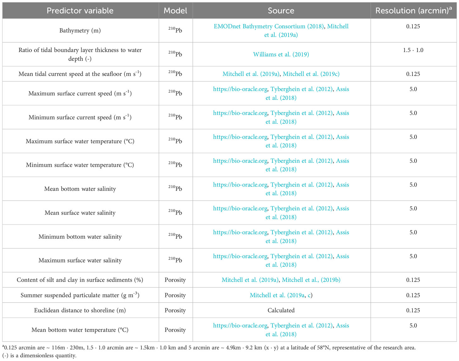
Table 1 List of predictor variables used in the ²¹⁰Pb rain rate and porosity models.

The predictor variables were gathered from various sources with unequal spatial extent, projection, and resolution. To create a stack of predictor layers, the predictor raster data were separately cropped to the area of interest depending on the initial resolution and projection. Subsequently, the predictors were reprojected to a common projection (Lambert azimuthal equal-area) and a resolution of 500 m by 500 m). The grid cells were aligned prior to modeling. The response data were averaged in those cases where more than one value fell into a grid cell of the predictor stack.

3.2 Machine learning models

The complete analysis was carried out in the free software environment for statistical computing and graphics R 4.2.3 (R Core Team, 2022) and RStudio 2023.03.0. This section provides an overview of the methodology used to spatially predict porosity and ²¹⁰Pb rain rates. We first give an overview of the workflow and its key features. The subsequent sections give more detailed information on the algorithms and R packages that were used.

3.2.1 Overview

The goal of this study is to determine the spatial distribution of a variable in a specific area. However, only a limited number of precise measurements of this variable is at our disposal. The task is therefore to estimate the variable at unsampled locations. This can be achieved by spatial prediction, which is the estimation of unknown quantities based on sample data and assumptions regarding the form of the trend and its variance and spatial correlation (Bivand et al., 2008). There are different types of spatial prediction models such as deterministic (e.g., inverse distance weighted interpolation) and stochastic methods (e.g., kriging). Here, we opted for a data-driven machine learning approach, because such models are flexible, can fit nonlinear and complex relationships, and do not need to satisfy strict statistical assumptions as opposed to stochastic models. In addition, such approaches allow users to quantify the uncertainty in the predictions.

Machine learning spatial models make predictions based on learned relationships between the variable to be predicted (response variable) and predictor variables, which exist with better coverage over the area of interest. Initially, it might be prudent to select a wide range of potentially relevant predictor variables, ideally based on a conceptual model (Guisan and Zimmermann, 2000) of the environmental system to be modeled. It is, however, generally recommended to limit the number of predictor variables that are finally used for modeling, as the predictive power decreases with an increase in the number of predictor variables given a fixed number of response data points (Hughes, 1968). The aims of variable selection are threefold: (1) to improve the prediction performance, (2) to enable faster predictions, and (3) to increase the interpretability of the model (Guyon and Elisseeff, 2003). Here, we use a forward selection approach whereby the model performance of various combinations of predictors is determined. Starting with combinations of two predictors, the number of predictors is increased until the model performance increases no longer.

Cross-validation is usually employed for model tuning and predictor variable selection. A frequently used scheme is k-fold cross-validation, whereby the dataset is randomly partitioned into k parts (folds) of approximately equal size. A single fold is retained for validating the model, while the remaining k - 1 folds are used to train the model. This is repeated k times, such that every fold serves as validation data once. The performance of a trained model can then be tested based on independent data not used for model building. However, truly independent test data are rarely available due to the costs of collecting sample data offshore. Holding back a fraction (usually 20-50%) of the data from model building and using this dataset for model testing might sometimes be an alternative. However, this requires a sufficiently large dataset. Additionally, a single split into training and test data might be unrepresentative and may provide misleading information about estimates and their uncertainty (Lyons et al., 2018). Because of these limitations, k-fold cross-validation is frequently used for model validation.

The use of machine learning algorithms in spatial prediction has strongly increased in recent years due to the advantages mentioned above and the seemingly high performance that is frequently achieved. However, it has been shown that model performance indicators might be inflated when spatial autocorrelation in the data is ignored (Ploton et al., 2020). To account for this, spatially separated folds can be generated for cross-validation. This is achieved by separating the sample data into spatial blocks of a size that accounts for spatial autocorrelation in the data. The blocks are subsequently randomly assigned to folds (Valavi et al., 2019).

Sampling design should be an integral part of spatial prediction and modeling to ensure good coverage of the environmental and geographic space (Biswas and Zhang, 2018). However, due to the costs of obtaining new sample data, making use of existing data stored in databases is crucial. This does mean that the set of sampling stations used for modeling rarely constitutes an optimal sampling design. Tools exist to gain insights to what extent the existing sample data deviates from an optimal design. Diesing (2020) provided plots that allow to assess to what extent the selected samples cover the environmental space of the predictor variables. Meyer and Pebesma (2022) compared the distributions of the spatial distances of sample data to their nearest neighbor with the distribution of distances from all points of prediction locations within an area of interest to the nearest sample data point. They showed that in the case of a spatially random sample dataset, which is a preferred design for spatial prediction, the two distribution curves overlap to a large extent. Model performance can be estimated with a random cross-validation in such a case. Conversely, clustered sample datasets show nearest neighbor distances between samples that are shorter than the distances from the prediction locations to the nearest sample data point. Spatial cross-validation is advised to derive realistic estimates of model performance.

Another way of accounting for limitations in the distribution of the sample data is to estimate the area in which the predictive model is valid. This area of applicability (AOA) of a model is defined as the area where the model was enabled to learn about relationships based on the training data, and where the estimated cross-validation performance holds. To delineate the AOA, a dissimilarity index (DI) is initially calculated. The DI is based on distances to the training data in the multidimensional predictor variable space. To account for the relevance of predictor variables responsible for prediction patterns variables are weighted by the model-derived variable importance scores prior to distance calculation. The AOA is then derived by applying a threshold based on the DI observed in the training data using cross-validation (Meyer and Pebesma, 2021).

3.2.2 Quantile regression forests

The QRF algorithm (Meinshausen, 2006) was selected to generate spatial predictions of porosity and ²¹⁰Pb rain rates. QRF can be seen as an extension of the random forest (RF) algorithm (Breiman, 2001), which has shown high predictive accuracy in several studies across various research domains (Prasad et al., 2006; Mutanga et al., 2012; Oliveira et al., 2012; Huang et al., 2014). The RF is an ensemble technique that creates regression trees using the predictor and response data. Each tree is constructed from a bootstrapped sample and a random subset of the predictor variables is used at each split in the tree-building process, making every tree in the forest unique. Individually, each tree in the forest may be a poor predictor and any combination of two trees can give different predictions. However, by aggregating the predictions over many uncorrelated trees, prediction variance is reduced, and accuracy is improved (James et al., 2013). RF can handle a large number of predictor variables, is insensitive to the inclusion of noisy predictors, can be used without extensive parameter tuning, and makes no assumptions regarding the shape of distributions of the response or predictor variables (Cutler et al., 2007). While RF outputs the mean over many regression trees to make an ensemble prediction, the QRF algorithm also returns the whole distribution of the response variable, based on which other measures of central tendency (e.g. median) and prediction uncertainty can be obtained. Following common practice in the global soil mapping community (Arrouays et al., 2014; Heuvelink, 2014), we used the 90% prediction interval (PI90) as a measure of spatially explicit uncertainty. PI90 gives the range of values within which the true value is expected to occur nine times out of ten, with a one in twenty probability for each of the two tails (Arrouays et al., 2014). It is defined as:

$\begin{array}{ll}\text{PI}90={\text{ q}}_{0.95}-{\text{q}}_{0.05}& (3)\end{array}$

with q_0.95 and q_0.05 being the 0.95 and 0.05 quantiles of the distribution, respectively. We chose the median as a measure of central tendency, as the conditional distributions were expected to be non-normal, and the median was not affected by extreme outliers.

As RF, and by extension QRF, has been shown to perform well without extensive parameter tuning (Cutler et al., 2007), we only carried out limited parameter tuning. The number of variables to consider at any given split (m_try) was tuned as part of the forward feature selection (see below). It is usually sufficient to set the number of trees in the forest (n_tree) to a high value; 500 was selected in this case.

3.2.3 Predictor variable selection

Predictor variable selection can be achieved in different ways. Here, we chose forward feature (variable) selection as implemented in the package “CAST” (Meyer et al., 2018). The algorithm first trained the models based on all possible combinations of two predictor variables. The best combination was retained and tested for the best performance with a third variable. Additional variables are added until the performance stops to increase. The model performance was calculated as R² using a spatial cross-validation scheme. Processing time increased with the number of predictors and response data points. The number of observations in the ²¹⁰Pb dataset was sufficiently small to run the forward feature selection on all predictor variables. However, it was decided to run a predictor variable pre-selection in the case of the porosity model. This pre-selection process first only retained important variables that performed better than random variables using the Boruta algorithm (Kursa and Rudnicki, 2010). In a second step, a de-correlation analysis was carried out to limit the collinearity. This was achieved with the “vifcor” function of the package “usdm” (Naimi et al., 2014). The function required a correlation threshold and the predictor variables as input to calculate variance inflation factors (VIF) of the predictors. The correlation threshold was stepwise decreased from 1 with a step size of 0.01 and predictors with a VIF ≥ 5 were removed. This process was repeated until the VIFs of all predictors were below 5 to avoid a problematic amount of collinearity (James et al., 2013).

A full list of the predictor variables that were selected by the models is provided in Table 1.

3.2.4 Spatial cross-validation

The estimation of model performance was based on k-fold cross-validation, whereby the response data were split into k folds. The model was built on k - 1 folds and validated against the fold which was not used for model building. This process was repeated k times, where k was set to 3. In the case of spatially clustered data, spatial autocorrelation might lead to inflated estimates of model performance (Roberts et al., 2017; Ploton et al., 2020). Folds therefore needed to be spatially separated and this was achieved with the function “cv_spatial” of the package “blockCV” (Valavi et al., 2019). The block size was initially determined by estimating the spatial autocorrelation range of the response data with the “automap package” (Hiemstra et al., 2009). The distance functions of the sample-to-sample, prediction-to-sample, and cross-validation distances were plotted with the “plot_geodist” function of “CAST” (Meyer and Pebesma, 2021) and the block size was altered by applying a multiplier to the spatial autocorrelation range until there was a visual agreement between the distance functions of the prediction-to-sample and cross-validation distances.

The performances of the final models were assessed based on the explained variance (R²) and the root mean square error (RMSE). Correlation plots between measured and predicted data are shown in the supplement (Figures S1, S2).

3.2.5 Area of applicability

We estimate the area of applicability (AOA) of the two models with the “aoa” function of the package “CAST” (Meyer and Pebesma, 2020). The spatial predictions and areawide quantifications presented in this study refer to the joint AOA of both the porosity and ²¹⁰Pb rain rate models, which spans an area of 21,270 km².

3.3 Calculation of MAR

In each grid cell of the model, predicted porosities were multiplied with existing spatial data of sedimentation rates (Diesing et al., 2021) to determine the spatial distribution of MAR:

$\begin{array}{ll} \text{MAR}={\text{ρ}}_{\text{DB}}·\text{SR }& (4)\end{array}$

where ρ_DB is the dry bulk density (Equation 2) and SR is the sedimentation rate.

Uncertainties for MAR (u(MAR)) were propagated by the uncertainties of ρ_DB and sedimentation rate from the literature (Diesing et al., 2021):

$\begin{array}{ll}\text{u}({\text{ρ}}_{\text{DB}})={\text{ρ}}_{\text{DB}}·\left(\frac{\text{u}(\mathrm{\varphi })}{1-\mathrm{\varphi }}\right)& (5)\end{array}$

$\begin{array}{ll}\text{u}(\text{MAR})=\text{MAR}·\sqrt{{(\frac{\text{u}({\text{ρ}}_{\text{DB}})}{{\text{ρ}}_{\text{DB}}})}^2+{(\frac{\text{u}(\text{SR})}{\text{SR}})}^2}& (6)\end{array}$

where u(ρ_DB), u(ϕ) and u(SR) are the uncertainties for dry bulk density, porosity, and sedimentation rates. The uncertainty of ds was assumed to be 0 g cm^-3. We note that the uncertainty calculation of porosity in this study differs from the approach for sedimentation rates in Diesing et al. (2021).

4 Results

4.1 Porosity

The four predictor variables for porosity selected by the model were the content of silt and clay in surface sediments, the distance to shoreline, mean bottom water temperatures and concentrations of suspended particulate matter during summer (Table 1). Predicted porosities varied between 42 and 86%, while the uncertainty ranged from 3 to 47% (Figure 3). The RMSE of the model was 5.1% and the R² was 0.8 (Figure S1). High porosities were observed in the basin below approximately 400 m water depth and low values along the coastlines at shallower water depths.

Figure 3

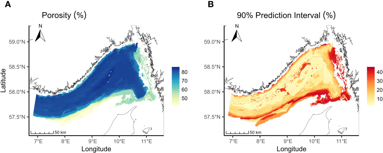
Figure 3 (A) Predicted spatial distribution of porosity and (B) associated uncertainty of the prediction.

4.2 Mass accumulation rate

Total MAR within the joint AOA of 21,270 km² was 34.7 Mt yr^-1 with an uncertainty of 39.8 Mt yr^-1 (Figure 4). The MAR varied between 0.01 and 0.38 g cm⁻² yr⁻¹ with the uncertainty ranging from 0.05 to 0.51 g cm⁻² yr⁻¹. High MARs were observed in a narrow belt between 300 and 350 m water depth in the southwestern part. The belt widens as it extends towards the northeastern part to up to 130 m water depth. Intermediate MAR occurred in the central Skagerrak basin, while lowest MAR were found in the southwestern part of the Skagerrak basin and along the Danish coastline at shallow water depth.

Figure 4

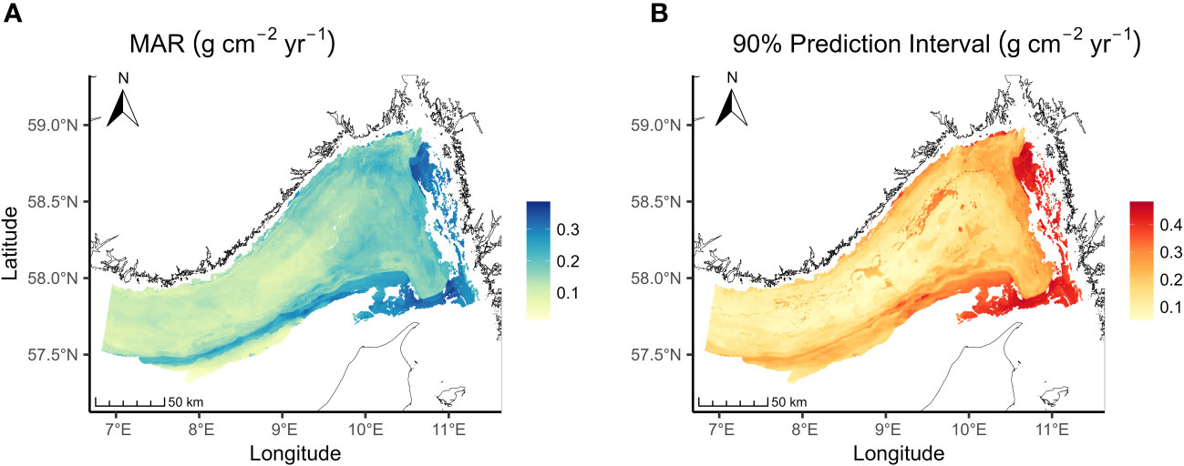
Figure 4 (A) Calculated spatial distribution of MAR and (B) associated uncertainty of the prediction.

4.3 ²¹⁰Pb rain rate

The predictor variables for the ²¹⁰Pb rain rate selected by the model were bathymetry, minimum and maximum surface current velocity and temperature, tidal current velocity at the seafloor, the ratio of tidal boundary layer thickness to water depth and minimum, maximum, as well as mean bottom and surface salinity. The predicted total ²¹⁰Pb rain rate in the joint AOA was 4.7 · 10¹⁴ dpm yr^-1 with an uncertainty of 9.3 · 10¹⁴ dpm yr^-1 (Figure 5). The ²¹⁰Pb rain rates varied between 0.3 and 5.4 dpm cm^-2 yr^-1 with uncertainties ranging from 1.0 to 6.8 dpm cm^-2 yr^-1. The model had an RMSE of 1.4 dpm cm^-2 yr^-1 and an R² of 0.41 (Figure S2). The highest rates were found in a belt structure along the basin between approximately 120 and 600 m water depth. Intermediate ²¹⁰Pb rain rates were predicted at the flanks of the high accumulation belt and in the central Skagerrak basin. The lowest rates were found along the Danish coastline at shallower water depths.

Figure 5

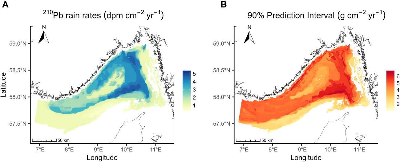
Figure 5 (A) Predicted spatial distribution of ²¹⁰Pb rain rates and (B) associated uncertainty of the prediction.

5 Discussion

5.1 Spatial distribution of porosity, MAR and ²¹⁰Pb rain rates

Certain patterns in the spatial variability of porosity, MAR, and ²¹⁰Pb rain rates can be explained by the hydrographic regime, indicating that the sediment transport broadly follows the general water circulation in the Skagerrak. Towards the northeastern part of the Skagerrak the current velocities decrease (van Weering et al., 1987, 1993), which promotes particle settling and contributes to the formation of belts characterized by high MAR and ²¹⁰Pb rain rates. In the case of MAR, the belt is located closer towards the coast at shallower water depths of up to 130 m. Since the MAR is a function of sedimentation rates and porosity (Equation 5), where lower porosities lead to higher MAR, the shift of the belt towards the coastline can be explained by the spatial variability of the porosity (Figure 3). Lower porosities close to the coastlines are indicative of coarser particle settling as a result of a more energetic hydrodynamic regime preventing the deposition of fine sediments. This relationship is consistent with the spatial grain size data in the Skagerrak (Stevens et al., 1996; Mitchell et al., 2019a). Conversely, high porosities found at greater water depths reflect the dominance of finer particles at the seafloor that settle due to reduced current velocities. The belt of elevated ²¹⁰Pb rain rates is situated in the area of high porosity and extends along the basin between 120 and 600 m water depth. The close relationship between ²¹⁰Pb rain rate and sediment transport is reflected in similar spatial patterns of the ²¹⁰Pb rain rates compared to previously published sedimentation rates (Diesing et al., 2021). Intermediate to high ²¹⁰Pb rain rates, sedimentation rates, and high porosities in large parts of the region suggest a substantial input of fine particles that may be delivered by lateral transport into the Skagerrak (see section 5.3).

In some areas along the coastlines at shallow water depths, the ²¹⁰Pb rain rates are comparable to, or lower than, the atmospheric ²¹⁰Pb input of 0.52 dpm cm^-2 yr^-1 (Peirson et al., 1966; Beks et al., 1998; Baskaran, 2011), indicating no lateral sediment input or net seafloor erosion in these areas (Figure 5). A possible explanation is the physical disturbance by waves and currents, leading to the resuspension of surface sediments at the seafloor. Given the exponential shape of a ²¹⁰Pb activity profile, continuous resuspension and subsequent relocation of ²¹⁰Pb-rich surface sediments could explain the depleted ²¹⁰Pb inventories at these sites. Considering the fishery activities in shallow waters and their impact on the seafloor in the North Sea and Skagerrak (ICES, 2020; Zhang et al., 2023¹), relocation of surface sediments by bottom trawling is another potential reason behind the ²¹⁰Pb loss. Supporting this hypothesis, disturbed ²¹⁰Pb profiles (Figure 2B) that may be indicative of bottom trawling (Spiegel et al., 2023) exclusively occur at shallow water depths< 400 m in line with the footprint of bottom trawling on the seafloor of the Skagerrak.

5.2 Total MAR and ²¹⁰Pb rain rates in the Skagerrak

The spatial distributions predicted by the machine learning models allowed for an estimate of the total MAR and ²¹⁰Pb rain rates in the Skagerrak. When integrating the rates across the joint AOA of the two models of 21270 km², the Skagerrak exhibits a MAR of 34.7 ± 39.8 Mt yr^-1 and a ²¹⁰Pb rain rate of 4.7 · 10¹⁴ ± 9.3 · 10¹⁴ dpm yr^-1. The presented rates are applicable for the last ~ 100 years, as the ²¹⁰Pb rain rates and the sedimentation rates used to calculate the MAR depend on ²¹⁰Pb activities in the sediment, of which roughly 97% is decayed after five times the half-life of ²¹⁰Pb (22.3 years). Hence, the results are representative as average values since the beginning of extensive human activities in the Skagerrak and North Sea (ICES, 2018, 2019, 2020; OSPAR, 2023) and can be used for comparisons with the sediment system of pre-industrial times. The presented MAR is comparable to previous estimates of 28 Mt yr^-1 and 46 Mt yr^-1 for the same area slightly differing in size (van Weering et al., 1987; de Haas and van Weering, 1997) and 19 Mt yr^-1 in the Norwegian part of the Skagerrak (Bøe et al., 1996). Their results were based on averaging sedimentation rate data and either assuming or measuring values for the porosity and density of dry solids to calculate area-wide MAR. Hence, the difference in the estimates is likely due to utilizing different data sets and upscaling methods.

5.3 Proportions of local and lateral ²¹⁰Pb and sediment inputs

By comparing ²¹⁰Pb rain rates at the seafloor with the atmospheric ²¹⁰Pb flux, it is possible to estimate the proportions of local and lateral ²¹⁰Pb inputs (DeMaster et al., 1986; Biscaye and Anderson, 1994), where the atmospheric flux is considered as the local source for ²¹⁰Pb. Assuming a constant spatial and temporal atmospheric ²¹⁰Pb flux of 0.52 dpm cm^-2 yr^-1 (Peirson et al., 1966; Beks et al., 1998; Baskaran, 2011) across the Skagerrak, the ²¹⁰Pb input by the atmosphere was calculated to be 1.1 · 10¹⁴ dpm yr^-1. Hence, the total ²¹⁰Pb rain rate of 4.7 · 10¹⁴ dpm yr^-1 is about 4 times the atmospheric input. The relative proportions of the local and lateral inputs are 24% and 76%, respectively. Consequently, lateral transport from outside the study area is the main source of ²¹⁰Pb in the Skagerrak. No details on the provenance of the lateral load can be derived from our evaluation. However, it is likely that a substantial portion stems from the southern and central North Sea as proposed by previous studies (Zöllmer and Irion, 1993; Bengtsson and Stevens, 1998; Irion and Zöllmer, 1999; Lepland et al., 2000).

de Haas and van Weering (1997) presented proportions of local and lateral organic matter inputs in the Skagerrak based on total organic carbon accumulation rates and primary production rates. They proposed that primary production only contributes about 10% to the total organic carbon accumulation rate, while the remaining 90% is transported laterally into the Skagerrak. We argue that the high affinity for particles and the otherwise conservative behavior make ²¹⁰Pb a favorable indicator for separating the lateral and local inputs of MAR. Despite its high particle reactivity, ²¹⁰Pb activities in deposits can be further affected by TOC contents (Xu et al., 2011; Anjum et al., 2017), the grain-size distribution (He and Walling, 1996) and sediment redistribution, making the assumption of a proportional relationship between ²¹⁰Pb and sediment fluxes in a natural system uncertain (Sanchez-Cabeza and Ruiz-Fernández, 2012). Such effects may become even more pronounced when considering that particle transport from the North Sea to the Skagerrak requires about two years (Hainbucher et al., 1987; Dahlgaard et al., 1995; Salomon et al., 1995). For instance, during transport from the North Sea, resuspension might introduce buried and already decayed ²¹⁰Pb to the lateral particle load. Conversely, the lateral load could be continuously recharged by fresh ²¹⁰Pb from the atmosphere. Decay during the transit is unlikely to significantly affect ²¹⁰Pb activities given the travel times and a ²¹⁰Pb half-life of 22.3 years. Since a detailed understanding of the relationship between long transit times, resuspension, and their impact on ²¹⁰Pb activities is unknown, the local and lateral sediment inputs we obtained represent a rough estimate. Assuming that the proportions of the local and lateral inputs derived from ²¹⁰Pb can be applied to the MAR, we calculated local and lateral sediment inputs of 8.2 and 26.5 Mt yr^-1, respectively. Local sediment sources usually constitute aeolian input and primary production. Considering primary production rate estimates of 90 - 190 g m^-2 yr^-1 in the Skagerrak (Anton et al., 1993; Meyenburg and Liebezeit, 1993; Heilmann et al., 1994; Richardson and Heilmann, 1995; Skogen et al., 1995; de Haas and van Weering, 1997; Skogen and Søiland, 2006), multiplication with the AOA yields a primary production of 1.9 - 4.0 Mt yr^-1 in the research area. Hence, our results indicate that aeolian inputs account for a significant fraction of the local input. However, there exist significant uncertainties in both the earlier estimates and in our ²¹⁰Pb-based calculations. Furthermore, previous studies indicated substantial temporal variability of primary production rates in the Skagerrak (Binczewska et al., 2018; Louchart et al., 2022). Hence, a more comprehensive approach, such as the application of organic carbon diagenetic modeling, is required to constrain the role of primary production in the local sediment input.

5.4 Tentative sediment budget of the North Sea

Based on our updated estimate on MAR and the existing literature, we derived a tentative sediment budget for the North Sea (Figure 6). Minor contributors to the sediment budget (< 3 Mt yr^-1) such as the Baltic Current input or sediment extraction were not considered in this budget, as their sum constituted only a small fraction of the overall sediment budget and sources and sinks of these minor contributors mostly balance out (Oost et al., 2021). Total sediment input into the North Sea amounts to 44 - 78 Mt yr^-1. The main contributors include sediment transport via the North Atlantic (Eisma and Irion, 1988; Puls et al., 1997; Eisma, 2009), the Dover Strait (McManus and Prandle, 1997; Fettweis et al., 2007; Eisma, 2009), cliff erosion along the UK coastline (Eisma and Irion, 1988; Puls et al., 1997), riverine inputs (Eisma and Irion, 1988) and seafloor erosion (Eisma and Irion, 1988; Van Alphen, 1990; ICONA, 1992). Total sediment outputs at depocenters in the North Sea and by the outflow to the North Atlantic are 88 Mt yr^-1. Of that, 35 Mt yr^-1 are deposited in the Skagerrak, supporting the notion that this region is the main depocenter for sediments from the North Sea. The Wadden Sea, in the southern and central North Sea, acts as another major sediment sink and traps approximately 11 Mt of the total sediment input annually (Oost et al., 2021). Furthermore, substantial MAR on the order of 28 Mt yr^-1 has been previously reported in the Norwegian Trench (de Haas et al., 1996). The remainder of 14 Mt yr^-1 that is not deposited at the seafloor leaves the North Sea through the Norwegian Coastal Current (Eisma, 2009). The overview reveals an imbalance between sedimentary sources and sinks in the North Sea, with sinks exceeding the sources. It is important to note the substantial uncertainties associated with the presented estimates, which may explain the observed imbalance. However, we further emphasize that the riverine inputs play a relatively minor role, while the particle transport through the northern Atlantic entrance and the Dover Straight are the major sediment sources for the North Sea. Most of the suspended load carried by both of these channels is probably supplied by erosion at coastlines surrounding the North Sea region. Recent studies have demonstrated that coastal erosion is a more dominant source than previously thought in the European seas (Regard et al., 2022) including the Baltic Sea (Wallmann et al., 2022). Hence, we suggest that current estimates of the channel inputs might be underestimated and could potentially close the sediment budget in the North Sea. The tentative North Sea sediment budget demonstrates the need to constrain the quantities of the different major sediment pathways for a comprehensive sediment budget in the North Sea.

Figure 6

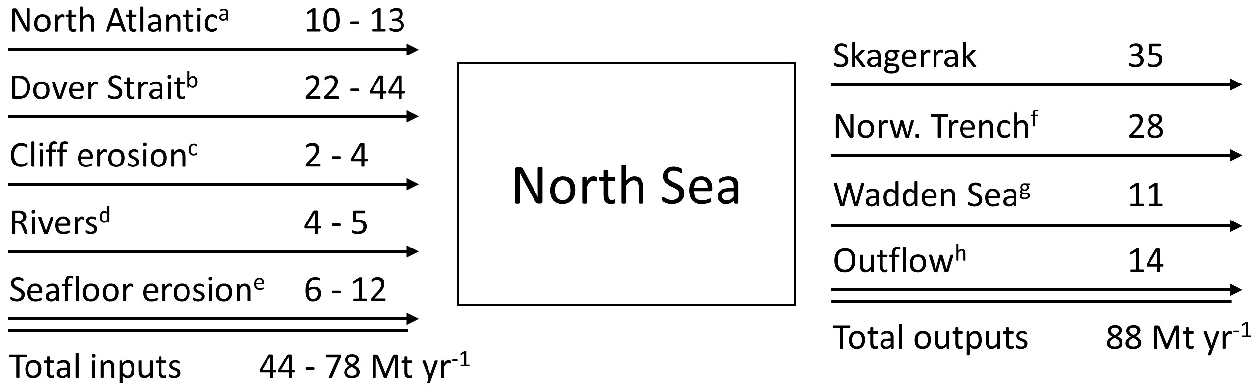
Figure 6 Tentative sediment budget for the North Sea. The major contributors to the sediment input include transport from (a) the North Atlantic (Eisma and Irion, 1988; Puls et al., 1997; Eisma, 2009) and (b) the Dover Strait (McManus and Prandle, 1997; Fettweis et al., 2007; Eisma, 2009), (c) cliff erosion (Eisma and Irion, 1988), (d) riverine input (Eisma and Irion, 1988) and (e) seafloor erosion (Eisma and Irion, 1988; Van Alphen, 1990; ICONA, 1992). Sediment outputs include deposition in the Skagerrak (this study), (f) the Norwegian Trench (de Haas et al., 1996) and (g) the Wadden Sea (Oost et al., 2021) and (h) outflow towards the North Atlantic (Eisma, 2009). All numbers are given in million tons of sediment per year.

5.5 Model appraisal, limitations, and future directions

We applied a machine learning approach to spatially predict sediment porosity and ²¹⁰Pb rain rates in the Skagerrak, while previous studies employed averaging to scale up individual data points in the Skagerrak (van Weering et al., 1987; Bøe et al., 1996; de Haas et al., 1996; de Haas and van Weering, 1997). We opted for machine learning as it has been previously demonstrated to be successful in predicting sedimentation rates and organic carbon densities in the same region (Diesing et al., 2021). Moreover, the machine learning approach shows principal advantages over averaging: (1) Machine learning yields spatially explicit results that can be displayed as maps. This allowed us to identify differences in the spatial patterns of MAR and ²¹⁰Pb rain rate, which were presented in section 5.1. In contrast, upscaling by averaging would yield one value applicable to the whole area, but without information about spatial variability. (2) The uncertainty of the predictions was assessed in a robust and spatially explicit way. Previous studies, as cited above, have provided estimates of the sediment accumulation, but no uncertainty has been given. (3) Although not investigated here, it is generally possible to explore the relationships between the response variable and the predictor variables with tools like variable importance and partial dependence plots (Hastie et al., 2009). This might help improve model building and understanding of the driving forces of the spatial patterns of the variable under consideration.

Although high uncertainties were calculated, it is important to keep in mind the definition of uncertainty we used (Equation 3). The PI90 gives the range of values within which the true value is expected to occur in 90% percent of the cases. Other studies have used the standard deviation (Diesing et al., 2021), a conformal prediction methodology (Restreppo et al., 2021) or none (Mitchell et al., 2021), leading to lower estimated uncertainties. Additionally, the propagation of uncertainties when calculating MAR (Equation 6) has increased the associated uncertainty estimates. This could be alleviated by directly predicting the MAR. However, this would require sufficient stations where sedimentation rates and dry bulk density or porosity have been measured.

General difficulties associated with sediment budgeting have been discussed in the literature (Brown et al., 2009; Parsons, 2012; Walton et al., 2012). Uncertainties include data availability, data quality and the applied upscaling approach. In our study, it was not possible to quantitatively address uncertainties owing to the data quality of the predictor and response variables, as measurement errors were rarely reported, and different sampling strategies and measurement techniques were applied in the complied literature. Therefore, improving the model performance and reducing the uncertainties was largely dependent on the available amount of response data and how the stations are distributed in space. Ideally, one should design a sampling survey prior to modeling in a way that optimizes the coverage of the samples in the study area. This could be achieved by, e.g., a simple random design (Meyer and Pebesma, 2022). However, data collection at sea is time and resource-consuming, and not making use of existing datasets would be a wasteful practice. We therefore followed the advice of Meyer and Pebesma (2021) and estimated the AOA of our models. The AOA results could be used for directing future sampling surveys to areas where the environment has not been sufficiently captured (Figure 2). Such a strategy would allow collecting additional data in an informed way to reduce uncertainties in the spatial distributions.

Predictor variables affected the performance based on their predictive capability, data quality and spatial resolution. A wide set of spatial data was available in the Skagerrak, enabling us to test their potential as predictors and ultimately providing a sufficient amount for the machine learning model. However, most of these predictors originate from the Bio-ORACLE global dataset (Tyberghein et al., 2012; Assis et al., 2018) with a spatial resolution of 5 arcmin, limiting the resolution of the model’s grid and its ability to consider fine-scale heterogeneities below the resolution of the raster stack. Hence, additional high-quality data on predictor variables could improve the predictive capability of the machine learning models to constrain the presented spatial distributions of porosity, MAR and ²¹⁰Pb rain rates.

6 Conclusion

In this study, we present the spatial distributions of porosity, ²¹⁰Pb rain rates and mass accumulation rates (MAR) in the Skagerrak based on machine learning. High MAR and ²¹⁰Pb rain rates are observed within two similar belt structures. The MAR belt is situated at shallower water depths given lower porosities towards the coast, while the ²¹⁰Pb belt extends along the basin. The calculated areawide MAR is 34.7 ± 39.8 Mt yr^-1 and ²¹⁰Pb rain rate is 4.7 · 10¹⁴ ± 9.3 · 10¹⁴ dpm yr^-1. By comparing the total ²¹⁰Pb rain rate to the atmospheric ²¹⁰Pb input, we calculate that 24% of the ²¹⁰Pb stems from the atmosphere, with the remainder of 76% being transported laterally into the Skagerrak. Considering the high particle reactivity of ²¹⁰Pb, these proportions are applied to the MAR to broadly estimate the local and lateral sediment inputs of 8.2 and 26.5 Mt yr^-1, respectively. We further present a tentative sediment budget for the North Sea, which reveals sedimentary sinks to be higher compared to the sources. Large uncertainties in the budget estimates may explain the imbalance. We further suggest that sediment inputs through the northern North Atlantic entrance and the Dover Straight could be underestimated. Although the machine learning approach currently represents one of the state-of-the-art methods for upscaling, large uncertainties in the predicted quantities persist. Incorporating more response data in areas that lie outside the AOA of the models could improve the predicted spatial distributions. The findings of this study contribute to the characterization of the Skagerrak region, particularly in terms of sediment mass balances and its role as the major depocenter for sediments from the North Sea. The spatial distributions can be used to validate ecosystem models and vice versa and provide a knowledge basis for resource management plans. Furthermore, the presented machine learning method for spatial upscaling can be applied to other regions to gain insights into areawide distribution patterns.

Data availability statement

The datasets presented in this study can be found in online repositories. The names of the repository/repositories and accession number(s) can be found below: 10.6084/m9.figshare.25076063.

Author contributions

TS: Writing – original draft. MD: Data curation, Methodology, Writing – review & editing. AD: Supervision, Writing – review & editing. NL: Writing – review & editing. MS: Writing – review & editing. SS: Writing – review & editing. CB: Writing – review & editing. MF: Writing – review & editing. HK: Writing – review & editing, Software, Visualization. CS: Writing – review & editing. KW: Funding acquisition, Project administration, Supervision, Writing – review & editing.

Funding

The author(s) declare financial support was received for the research, authorship, and/or publication of this article. Funding for this study was provided by the Federal Ministry of Education and Research, Germany, via the APOC project (03F0874B) – “Anthropogenic impacts on particulate organic carbon cycling in the North Sea”.

Acknowledgments

We thank the captain and crew of RV Alkor for supporting our research at sea, as well as our colleagues Bettina Domeyer, Anke Bleyer, Regina Surberg, Matthias Türk and Asmus Petersen for their help onboard during the cruise AL561 and in the GEOMAR laboratories. We further wish to thank Andreas Neumann from the Helmholtz-Zentrum Hereon for providing sediment samples of the RV Alkor cruise AL557. We would also like to acknowledge Matthias Moros from the Leibniz-Institut für Ostseeforschung Warnemünde, Bernd Kopka and Marvin Blaue from the Laboratory for Radioisotopes at the University of Göttingen, Christian Kunze and Robert Arndt from the IAF Dresden and Hendrik Wolschke from the Helmholtz-Zentrum Hereon for the ²¹⁰Pb analyses. Funding for this study was provided by the Federal Ministry of Education and Research, Germany, via the APOC project (03F0874B) – “Anthropogenic impacts on particulate organic carbon cycling in the North Sea”.

Conflict of interest

The authors declare that the research was conducted in the absence of any commercial or financial relationships that could be construed as a potential conflict of interest.

The author(s) declared that they were an editorial board member of Frontiers, at the time of submission. This had no impact on the peer review process and the final decision.

Publisher’s note

All claims expressed in this article are solely those of the authors and do not necessarily represent those of their affiliated organizations, or those of the publisher, the editors and the reviewers. Any product that may be evaluated in this article, or claim that may be made by its manufacturer, is not guaranteed or endorsed by the publisher.

Supplementary material

The Supplementary Material for this article can be found online at: https://www.frontiersin.org/articles/10.3389/fmars.2024.1331102/full#supplementary-material

Footnotes

1. ^ Zhang, W., Porz, L., Yilmaz, R., Wallmann, K., Spiegel, T., Neumann, A., et al. (2023). Intense and persistent bottom trawling impairs long-term carbon storage in shelf sea sediments. doi: 10.21203/rs.3.rs-3313118/v1.

References

Alperin M. J., Suayah I. B., Benninger L. K., Martens C. S. (2002). Modern organic carbon burial fluxes, recent sedimentation rates, and particle mixing rates from the upper continental slope near Cape Hatteras, North Carolina (USA). Deep Sea Res. Part II Top. Stud. Oceanogr. 49, 4645–4665. doi: 10.1016/S0967-0645(02)00133-9

CrossRef Full Text | Google Scholar

Anjum R., Gao J., Tang Q., He X., Zhang X., Long Y., et al. (2017). Linking sedimentary total organic carbon to 210 Pb ex chronology from Changshou Lake in the Three Gorges Reservoir Region, China. Chemosphere 174, 243–252. doi: 10.1016/j.chemosphere.2017.01.060

PubMed Abstract | CrossRef Full Text | Google Scholar

Anton K. K., Liebezeit G., Rudolph C., Wirth H. (1993). Origin, distribution and accumulation of organic carbon in the Skagerrak. Mar. Geol. 111, 287–297. doi: 10.1016/0025-3227(93)90136-J

CrossRef Full Text | Google Scholar

Arrouays D., Grundy M. G., Hartemink A. E., Hempel J. W., Heuvelink G. B. M., Hong S. Y., et al. (2014). “GlobalSoilMap,” in Advances in Agronomy (Elsevier), 93–134. doi: 10.1016/B978-0-12-800137-0.00003-0

CrossRef Full Text | Google Scholar

Assis J., Tyberghein L., Bosch S., Verbruggen H., Serrão E. A., De Clerck O., et al. (2018). Bio-ORACLE v2.0: Extending marine data layers for bioclimatic modelling. Glob. Ecol. Biogeogr. 27, 277–284. doi: 10.1111/geb.12693

CrossRef Full Text | Google Scholar

Baskaran M. (2011). Po-210 and Pb-210 as atmospheric tracers and global atmospheric Pb-210 fallout: a Review. J. Environ. Radioact. 102, 500–513. doi: 10.1016/j.jenvrad.2010.10.007

PubMed Abstract | CrossRef Full Text | Google Scholar

Beks J. P. (2000). Storage and distribution of plutonium, 241Am, 137Cs and 210Pbxs in North Sea sediments. Cont. Shelf Res. 20, 1941–1964. doi: 10.1016/S0278-4343(00)00057-1

CrossRef Full Text | Google Scholar

Beks J. P., Eisma D., van der Plicht J. (1998). A record of atmospheric 210Pb deposition in The Netherlands. Sci. Total Environ. 222, 35–44. doi: 10.1016/S0048-9697(98)00289-7

CrossRef Full Text | Google Scholar

Bengtsson H., Stevens R. L. (1998). Source and grain-size influences upon the clay mineral distribution in the Skagerrak and northern Kattegat. Clay Miner. 33, 3–13. doi: 10.1180/000985598545381

CrossRef Full Text | Google Scholar

Binczewska A., Risebrobakken B., Polovodova Asteman I., Moros M., Tisserand A., Jansen E., et al. (2018). Coastal primary productivity changes over the last millennium: a case study from the Skagerrak (North Sea). Biogeosciences 15, 5909–5928. doi: 10.5194/bg-15-5909-2018

CrossRef Full Text | Google Scholar

Biscaye P. E., Anderson R. F. (1994). Fluxes of particulate matter on the slope of the southern Middle Atlantic Bight: SEEP-II. Deep Sea Res. Part II Top. Stud. Oceanogr. 41, 459–509. doi: 10.1016/0967-0645(94)90032-9

CrossRef Full Text | Google Scholar

Biswas A., Zhang Y. (2018). Sampling designs for validating digital soil maps: A review. Pedosphere 28, 1–15. doi: 10.1016/S1002-0160(18)60001-3

CrossRef Full Text | Google Scholar

Bivand R. S., Pebesma E. J., Gómez-Rubio (2008). Applied Spatial Data Analysis with R (New York, NY: Springer New York). doi: 10.1007/978-0-387-78171-6

CrossRef Full Text | Google Scholar

Bøe R., Rise L., Thorsnes T., De Haas H., Saether O. M., Kunzendortf H. (1996). Sea-bed sediments and sediment accumulation rates in the Norwegian part of the Skagerrak. Geol Bull. 430, 75–84.

Google Scholar

Breiman L. (2001). Random forests. Mach. Learn. 45, 5–32. doi: 10.1023/A:1010933404324

CrossRef Full Text | Google Scholar

Brown A. G., Carey C., Erkens G., Fuchs M., Hoffmann T., Macaire J.-J., et al. (2009). From sedimentary records to sediment budgets: Multiple approaches to catchment sediment flux. Geomorphology 108, 35–47. doi: 10.1016/j.geomorph.2008.01.021

CrossRef Full Text | Google Scholar

Cochran J. K., McKibbin-Vaughan T., Dornblaser M. M., Hirschberg D., Livingston H. D., Buesseler K. O. (1990). 210Pb scavenging in the North Atlantic and North Pacific Oceans. Earth Planet. Sci. Lett. 97, 332–352. doi: 10.1016/0012-821X(90)90050-8

CrossRef Full Text | Google Scholar

Cutler D. R., Edwards T. C., Beard K. H., Cutler A., Hess K. T., Gibson J., et al. (2007). RANDOM FORESTS FOR CLASSIFICATION IN ECOLOGY. Ecology 88, 2783–2792. doi: 10.1890/07-0539.1

PubMed Abstract | CrossRef Full Text | Google Scholar

Dahlgaard H., Herrmann J., Salomon J. C. (1995). A tracer study of the transport of coastal water from the English Channel through the German Bight to the Kattegat. J. Mar. Syst. 6, 415–425. doi: 10.1016/0924-7963(95)00017-J

CrossRef Full Text | Google Scholar

De Groot S. J. (1986). Marine sand and gravel extraction in the North Atlantic and its potential environmental impact, with emphasis on the North Sea. Ocean Manage. 10, 21–36. doi: 10.1016/0302-184X(86)90004-1

CrossRef Full Text | Google Scholar

de Haas H., Okkels E., De Haas, van Weering (1996). Recent sediment accumulation in the Norwegian Channel, North Sea. Geol Bull. 430, 57–65.

Google Scholar

de Haas H., van Weering T. C. E. (1997). Recent sediment accumulation, organic carbon burial and transport in the northeastern North Sea. Mar. Geol. 136, 173–187. doi: 10.1016/S0025-3227(96)00072-2

CrossRef Full Text | Google Scholar

DeMaster D. J., Kuehl S. A., Nittrouer C. A. (1986). Effects of suspended sediments on geochemical processes near the mouth of the Amazon River: examination of biological silica uptake and the fate of particle-reactive elements. Cont. Shelf Res. 6, 107–125. doi: 10.1016/0278-4343(86)90056-7

CrossRef Full Text | Google Scholar

Deng L., Bölsterli D., Kristensen E., Meile C., Su C.-C., Bernasconi S. M., et al. (2020). Macrofaunal control of microbial community structure in continental margin sediments. Proc. Natl. Acad. Sci. 117, 15911–15922. doi: 10.1073/pnas.1917494117

CrossRef Full Text | Google Scholar

Diesing M. (2020). Deep-sea sediments of the global ocean. Earth Syst. Sci. Data 12, 3367–3381. doi: 10.5194/essd-12-3367-2020

CrossRef Full Text | Google Scholar

Diesing M., Thorsnes T., Bjarnadóttir L. R. (2021). Organic carbon densities and accumulation rates in surface sediments of the North Sea and Skagerrak. Biogeosciences 18, 2139–2160. doi: 10.5194/bg-18-2139-2021

CrossRef Full Text | Google Scholar

Eisma D. (2009). “Supply and deposition of suspended matter in the North Sea,” in Holocene Marine Sedimentation in the North Sea Basin. Eds. Nio S.-D., Shüttenhelm R. T. E., Van Weering T. (Blackwell Publishing Ltd., Oxford, UK), 415–428. doi: 10.1002/9781444303759.ch29

CrossRef Full Text | Google Scholar

Eisma D., Irion G. (1988). “Suspended matter and sediment transport,” in Pollution of the North Sea. Eds. Salomons W., Bayne B. L., Duursma E. K., Förstner U. (Springer Berlin Heidelberg, Berlin, Heidelberg), 20–35. doi: 10.1007/978-3-642-73709-1_2

CrossRef Full Text | Google Scholar

EMODnet Bathymetry Consortium (2018). EMODnet Digital Bathymetry (DTM 2018). doi: 10.12770/18FF0D48-B203-4A65-94A9-5FD8B0EC35F6

CrossRef Full Text | Google Scholar

Erlenkeuser H. (1985). Distribution of 210Pb with depth in core GIK 15530-4 from the Skagerrak. Nor. Geol. Tidsskr. 65, 27–34.

Google Scholar

Erlenkeuser H., Pederstad K. (1984). Recent sediment accumulation in Skagerrak as depicted by 210pb-dating. Nor. Geol. Tidsskr. 18, 135–152.

Google Scholar

Ferdelman T. G. (2005a). Radionuclides of caesium, potassium, lead and radium of sediment core GT03-71RL. doi: 10.1594/PANGAEA.319835

CrossRef Full Text | Google Scholar

Ferdelman T. G. (2005b). Radionuclides of caesium, potassium, lead and radium of sediment core GT03-72RL. doi: 10.1594/PANGAEA.319836

CrossRef Full Text | Google Scholar

Ferdelman T. G. (2005c). Radionuclides of caesium, potassium, lead and radium of sediment core GT03-68RL. doi: 10.1594/PANGAEA.319834

CrossRef Full Text | Google Scholar

Fettweis M., NeChad B., Van Den Eynde D. (2007). An estimate of the suspended particulate matter (SPM) transport in the southern North Sea using SeaWiFS images, in situ measurements and numerical model results. Cont. Shelf Res. 27, 1568–1583. doi: 10.1016/j.csr.2007.01.017

CrossRef Full Text | Google Scholar

Guisan A., Zimmermann N. E. (2000). Predictive habitat distribution models in ecology. Ecol. Model. 135, 147–186. doi: 10.1016/S0304-3800(00)00354-9

CrossRef Full Text | Google Scholar

Guyon I., Elisseeff A. (2003). An introduction to variable and feature selection. J. Mach. Learn. Res. 3, 1157–1182.

Google Scholar

Hainbucher D., Pohlmann T., Backhaus J. (1987). Transport of conservative passive tracers in the North Sea: first results of a circulation and transport model. Cont. Shelf Res. 7, 1161–1179. doi: 10.1016/0278-4343(87)90083-5

CrossRef Full Text | Google Scholar

Hastie T., Tibshirani R., Friedman J. (2009). The Elements of Statistical Learning, Springer Series in Statistics (New York, NY: Springer New York). doi: 10.1007/978-0-387-84858-7

CrossRef Full Text | Google Scholar

He Q., Walling D. E. (1996). Interpreting particle size effects in the adsorption of 137Cs and unsupported 210Pb by mineral soils and sediments. J. Environ. Radioact. 30, 117–137. doi: 10.1016/0265-931X(96)89275-7

CrossRef Full Text | Google Scholar

Heilmann J. P., Richardson K., Ærtebjerg G. (1994). Annual distribution and activity of phytoplankton in the Skagerrak/Kattegat frontal region. Mar. Ecol. Prog. Ser. 112, 213–223. doi: 10.3354/meps112213

CrossRef Full Text | Google Scholar

Heinatz K., Scheffold M. I. E. (2023). A first estimate of the effect of offshore wind farms on sedimentary organic carbon stocks in the Southern North Sea. Front. Mar. Sci. 9. doi: 10.3389/fmars.2022.1068967

CrossRef Full Text | Google Scholar

Heuvelink G. (2014). “Uncertainty quantification of GlobalSoilMap products,” in GlobalSoilMap. Eds. Arrouays D., McKenzie N., Hempel J., De Forges A., McBratney A. (CRC Press), 335–340. doi: 10.1201/b16500-62

CrossRef Full Text | Google Scholar

Hiemstra P. H., Pebesma E. J., Twenhöfel C. J. W., Heuvelink G. B. M. (2009). Real-time automatic interpolation of ambient gamma dose rates from the Dutch radioactivity monitoring network. Comput. Geosci. 35, 1711–1721. doi: 10.1016/j.cageo.2008.10.011

CrossRef Full Text | Google Scholar

Huang Z., Siwabessy J., Nichol S. L., Brooke B. P. (2014). Predictive mapping of seabed substrata using high-resolution multibeam sonar data: A case study from a shelf with complex geomorphology. Mar. Geol. 357, 37–52. doi: 10.1016/j.margeo.2014.07.012

CrossRef Full Text | Google Scholar

Hughes G. (1968). On the mean accuracy of statistical pattern recognizers. IEEE Trans. Inf. Theory 14, 55–63. doi: 10.1109/TIT.1968.1054102

CrossRef Full Text | Google Scholar

ICES (2018). Greater North Sea Ecoregion ? Ecosystem overview. doi: 10.17895/ICES.PUB.4670

CrossRef Full Text | Google Scholar

ICES (2019). Working Group on the Effects of Extraction of Marine Sediments on the Marine Ecosystem (WGEXT). doi: 10.17895/ICES.PUB.5733

CrossRef Full Text | Google Scholar

ICES (2020). Greater North Sea ecoregion ? Fisheries overview, including mixed-fisheries considerations. doi: 10.17895/ICES.ADVICE.7605

CrossRef Full Text | Google Scholar

ICONA (1992). North Sea atlas: for Netherlands policy and management (Amsterdam: Stadsuitgeverij Amsterdam).

Google Scholar

Irion G., Zöllmer V. (1999). Clay mineral associations in fine-grained surface sediments of the North Sea. J. Sea Res. 41, 119–128. doi: 10.1016/S1385-1101(98)00041-0

CrossRef Full Text | Google Scholar

James G., Witten D., Hastie T., Tibshirani R. (2013). An Introduction to Statistical Learning, Springer Texts in Statistics (New York, NY: Springer New York). doi: 10.1007/978-1-4614-7138-7

CrossRef Full Text | Google Scholar

Krishnaswamy S., Lal D., Martin J. M., Meybeck M. (1971). Geochronology of lake sediments. Earth Planet. Sci. Lett. 11, 407–414. doi: 10.1016/0012-821X(71)90202-0

CrossRef Full Text | Google Scholar

Kristiansen T., Aas E. (2015). Water type quantification in the Skagerrak, the Kattegat and off the Jutland west coast. Oceanologia 57, 177–195. doi: 10.1016/j.oceano.2014.11.002

CrossRef Full Text | Google Scholar

Kursa M. B., Rudnicki W. R. (2010). Feature selection with the Boruta package. J. Stat. Software 36 (11), 1–13. doi: 10.18637/jss.v036.i11

CrossRef Full Text | Google Scholar

Lepland A., Sæther O., Thorsnes T. (2000). Accumulation of barium in recent Skagerrak sediments: sources and distribution controls. Mar. Geol. 163, 13–26. doi: 10.1016/S0025-3227(99)00104-8

CrossRef Full Text | Google Scholar

Louchart A., Lizon F., Claquin P., Artigas L. F., Tilstone G., Land P. (2022). “Pilot assessment on primary production,” in OSPAR 2023: The 2023 Quality Status Report for the North-East Atlantic (OSPAR Commission, London).

Google Scholar

Lyons M. B., Keith D. A., Phinn S. R., Mason T. J., Elith J. (2018). A comparison of resampling methods for remote sensing classification and accuracy assessment. Remote Sens. Environ. 208, 145–153. doi: 10.1016/j.rse.2018.02.026

CrossRef Full Text | Google Scholar

McManus J. P., Prandle D. (1997). Development of a model to reproduce observed suspended sediment distributions in the southern North Sea using Principal Component Analysis and Multiple Linear Regression. Cont. Shelf Res. 17, 761–778. doi: 10.1016/S0278-4343(96)00057-X

CrossRef Full Text | Google Scholar

Meinshausen N. (2006). Quantile regression forests. J. Mach. Learn Res. 7, 983–999.

Google Scholar

Meyenburg G., Liebezeit G. (1993). Mineralogy and geochemistry of a core from the Skagerrak/Kattegat boundary. Mar. Geol. 111, 337–344. doi: 10.1016/0025-3227(93)90139-M

CrossRef Full Text | Google Scholar

Meyer H., Pebesma E. (2020). Mapping (un)certainty of machine learning-based spatial prediction models based on predictor space distances. EGU General Assembly 2020. Online, 4–8 May 2020, EGU2020-8492. doi: 10.5194/egusphere-egu2020-8492

CrossRef Full Text | Google Scholar

Meyer H., Pebesma E. (2021). Predicting into unknown space? Estimating the area of applicability of spatial prediction models. Methods Ecol. Evol. 12, 1620–1633. doi: 10.1111/2041-210X.13650

CrossRef Full Text | Google Scholar

Meyer H., Pebesma E. (2022). Machine learning-based global maps of ecological variables and the challenge of assessing them. Nat. Commun. 13, 2208. doi: 10.1038/s41467-022-29838-9

PubMed Abstract | CrossRef Full Text | Google Scholar

Meyer H., Reudenbach C., Hengl T., Katurji M., Nauss T. (2018). Improving performance of spatio-temporal machine learning models using forward feature selection and target-oriented validation. Environ. Model. Software 101, 1–9. doi: 10.1016/j.envsoft.2017.12.001

CrossRef Full Text | Google Scholar

Mielck F., Hass H. C., Michaelis R., Sander L., Papenmeier S., Wiltshire K. H. (2019). Morphological changes due to marine aggregate extraction for beach nourishment in the German Bight (SE North Sea). Geo-Mar. Lett. 39, 47–58. doi: 10.1007/s00367-018-0556-4

CrossRef Full Text | Google Scholar

Mitchell P. J., Aldridge J., Diesing M. (2019a). Legacy data: how decades of seabed sampling can produce robust predictions and versatile products. Geosciences 9, 182. doi: 10.3390/geosciences9040182

CrossRef Full Text | Google Scholar

Mitchell P., Aldridge J., Diesing M. (2019b). Predictor variables and groundtruth samples for north-west European continental shelf quantitative sediment analysis. doi: 10.14466/CEFASDATAHUB.62

CrossRef Full Text | Google Scholar

Mitchell P., Aldridge J., Diesing M. (2019c). Quantitative sediment composition predictions for the north-west European continental shelf. doi: 10.14466/CEFASDATAHUB.63

CrossRef Full Text | Google Scholar

Mitchell P. J., Spence M. A., Aldridge J., Kotilainen A. T., Diesing M. (2021). Sedimentation rates in the Baltic Sea: A machine learning approach. Cont. Shelf Res. 214, 104325. doi: 10.1016/j.csr.2020.104325

CrossRef Full Text | Google Scholar

Morang A., Waters J. P., Khalil S. M. (2012). Gulf of Mexico regional sediment budget. J. Coast. Res. 60, 14–29. doi: 10.2112/SI_60_3

CrossRef Full Text | Google Scholar

Mutanga O., Adam E., Cho M. A. (2012). High density biomass estimation for wetland vegetation using WorldView-2 imagery and random forest regression algorithm. Int. J. Appl. Earth Obs. Geoinformation 18, 399–406. doi: 10.1016/j.jag.2012.03.012

CrossRef Full Text | Google Scholar

Naimi B., Hamm N. A. S., Groen T. A., Skidmore A. K., Toxopeus A. G. (2014). Where is positional uncertainty a problem for species distribution modelling? Ecography 37, 191–203. doi: 10.1111/j.1600-0587.2013.00205.x

CrossRef Full Text | Google Scholar

Nittrouer C. A., Sternberg R. W., Carpenter R., Bennett J. T. (1979). The use of Pb-210 geochronology as a sedimentological tool: Application to the Washington continental shelf. Mar. Geol. 31, 297–316. doi: 10.1016/0025-3227(79)90039-2

CrossRef Full Text | Google Scholar

Nozaki Y., Tsubota H., Kasemsupaya V., Yashima M., Naoko I. (1991). Residence times of surface water and particle-reactive 210Pb and 210Po in the East China and Yellow seas. Geochim. Cosmochim. Acta 55, 1265–1272. doi: 10.1016/0016-7037(91)90305-O

CrossRef Full Text | Google Scholar

Oliveira S., Oehler F., San-Miguel-Ayanz J., Camia A., Pereira J. M. C. (2012). Modeling spatial patterns of fire occurrence in Mediterranean Europe using Multiple Regression and Random Forest. For. Ecol. Manage. 275, 117–129. doi: 10.1016/j.foreco.2012.03.003

CrossRef Full Text | Google Scholar

Oost A., Colina Alonso A., Esselink P., Wang Z. B., van Kessel T., van Maren B. (2021). Where mud matters: towards a mud balance for the trilateral Wadden Sea Area: mud supply, transport and deposition (Leeuwarden: Wadden Academy).

Google Scholar

OSPAR (2023) OSPAR Quality Status Synthesis Report 2023. Available online at: oap.ospar.org.

Google Scholar

Otto L., Zimmerman J. T. F., Furnes G. K., Mork M., Saetre R., Becker G. (1990). Review of the physical oceanography of the North Sea. Neth. J. Sea Res. 26, 161–238. doi: 10.1016/0077-7579(90)90091-T

CrossRef Full Text | Google Scholar

Paetzel M., Schrader H., Bjerkli K. (1994). Do decreased trace metal concentrations in surficial skagerrak sediments over the last 15–30 years indicate decreased pollution? Environ. pollut. 84, 213–226. doi: 10.1016/0269-7491(94)90132-5

PubMed Abstract | CrossRef Full Text | Google Scholar

Parsons A. J. (2012). How useful are catchment sediment budgets? Prog. Phys. Geogr. Earth Environ. 36, 60–71. doi: 10.1177/0309133311424591

CrossRef Full Text | Google Scholar

Peirson D. H., Cambray R. S., Spicer G. S. (1966). Lead-210 and polonium-210 in the atmosphere. Tellus 18, 427–433. doi: 10.1111/j.2153-3490.1966.tb00254.x

CrossRef Full Text | Google Scholar

Ploton P., Mortier F., Réjou-Méchain M., Barbier N., Picard N., Rossi V., et al. (2020). Spatial validation reveals poor predictive performance of large-scale ecological mapping models. Nat. Commun. 11, 4540. doi: 10.1038/s41467-020-18321-y

PubMed Abstract | CrossRef Full Text | Google Scholar

Prasad A. M., Iverson L. R., Liaw A. (2006). Newer classification and regression tree techniques: bagging and random forests for ecological prediction. Ecosystems 9, 181–199. doi: 10.1007/s10021-005-0054-1

CrossRef Full Text | Google Scholar

Puls W., Heinrich H., Mayer B. (1997). Suspended particulate matter budget for the German Bight. Mar. pollut. Bull. 34, 398–409. doi: 10.1016/S0025-326X(96)00161-0

CrossRef Full Text | Google Scholar

R Core Team (2022). R: A language and environment for statistical computing (Vienna, Austria: R Foundation for Statistical Computing). Available at: https://www.R-project.org/.

Google Scholar

Regard V., Prémaillon M., Dewez T. J. B., Carretier S., Jeandel C., Godderis Y., et al. (2022). Rock coast erosion: An overlooked source of sediments to the ocean. Europe as an example. Earth Planet. Sci. Lett. 579, 117356. doi: 10.1016/j.epsl.2021.117356

CrossRef Full Text | Google Scholar

Restreppo G. A., Wood W. T., Graw J. H., Phrampus B. J. (2021). A machine-learning derived model of seafloor sediment accumulation. Mar. Geol. 440, 106577. doi: 10.1016/j.margeo.2021.106577

CrossRef Full Text | Google Scholar

Richardson K., Heilmann J. P. (1995). Primary production in the Kattegat: Past and present. Ophelia 41, 317–328. doi: 10.1080/00785236.1995.10422050

CrossRef Full Text | Google Scholar

Richardson M. D., Jackson D. R. (2017). “The seafloor,” in Applied Underwater Acoustics (Amsterdam: Elsevier), 469–552. doi: 10.1016/B978-0-12-811240-3.00008-4

CrossRef Full Text | Google Scholar

Roberts D. R., Bahn V., Ciuti S., Boyce M. S., Elith J., Guillera-Arroita G., et al. (2017). Cross-validation strategies for data with temporal, spatial, hierarchical, or phylogenetic structure. Ecography 40, 913–929. doi: 10.1111/ecog.02881

CrossRef Full Text | Google Scholar

Salomon J. C., Breton M., Guegueniat P. (1995). A 2D long term advection—dispersion model for the Channel and southern North Sea Part B: Transit time and transfer function from Cap de la Hague. J. Mar. Syst. 6, 515–527. doi: 10.1016/0924-7963(95)00021-G

CrossRef Full Text | Google Scholar

Sanchez-Cabeza J. A., Ruiz-Fernández A. C. (2012). 210Pb sediment radiochronology: An integrated formulation and classification of dating models. Geochim. Cosmochim. Acta 82, 183–200. doi: 10.1016/j.gca.2010.12.024

CrossRef Full Text | Google Scholar

Schmidt M. (2021). “Dynamics and variability of POC burial in depocenters of the North Sea (Skagerrak), Cruise No. AL561, 2.08.2021 – 13.08.2021, Kiel – Kiel, APOC,” in GEOMAR Helmholtz Centre for Ocean Research Kiel. AL561, 34 pp. doi: 10.3289/CR_AL561

CrossRef Full Text | Google Scholar

Skogen M. D., Søiland H. (2006). Environmental status of the Skagerrak and North Sea 2004.

Google Scholar

Skogen M. D., Svendsen E., Berntsen J., Aksnes D., Ulvestad K. B. (1995). Modelling the primary production in the North Sea using a coupled three-dimensional physical-chemical-biological ocean model. Estuar. Coast. Shelf Sci. 41, 545–565. doi: 10.1016/0272-7714(95)90026-8

CrossRef Full Text | Google Scholar

Spiegel T., Dale A. W., Lenz N., Schmidt M., Sommer S., Kalapurakkal H. T., et al. (2023). Biogenic silica cycling in the Skagerrak. Front. Mar. Sci. 10. doi: 10.3389/fmars.2023.1141448

CrossRef Full Text | Google Scholar

Ståhl H., Tengberg A., Brunnegård J., Bjørnbom E., Forbes T. L., Josefson A. B., et al. (2004). Factors influencing organic carbon recycling and burial in Skagerrak sediments. J. Mar. Res. 62, 867–907. doi: 10.1357/0022240042880873

CrossRef Full Text | Google Scholar

Stevens R. L., Bengtsson H., Lepland A. (1996). Textural provinces and transport interpretations with fine-grained sediments in the Skagerrak. J. Sea Res. 35, 99–110. doi: 10.1016/S1385-1101(96)90739-X

CrossRef Full Text | Google Scholar

Thomas H., Freund W., Mears C., Meckel E., Minutolo F., Nantke C., et al. (2022). ALKOR Scientific Cruise Report. The Ocean's Alkalinity - Connecting geological and metabolic processes and time-scales: mechanisms and magnitude of metabolic alkalinity generation in the North Sea Cruise No. AL557. Open Access. Alkor-Berichte, AL557. GEOMAR Helmholtz-Zentrum für Ozeanforschung Kiel, Kiel, Germany, 22 pp.

Google Scholar

Tyberghein L., Verbruggen H., Pauly K., Troupin C., Mineur F., De Clerck O. (2012). Bio-ORACLE: a global environmental dataset for marine species distribution modelling: Bio-ORACLE marine environmental data rasters. Glob. Ecol. Biogeogr. 21, 272–281. doi: 10.1111/j.1466-8238.2011.00656.x

CrossRef Full Text | Google Scholar

Valavi R., Elith J., Lahoz-Monfort J. J., Guillera-Arroita G. (2019). BlockCV: An r package for generating spatially or environmentally separated folds for k-fold cross-validation of species distribution models. Methods Ecol. Evol. 10, 225–232. doi: 10.1111/2041-210X.13107

CrossRef Full Text | Google Scholar

Van Alphen J. S. L. J. (1990). A mud balance for Belgian-Dutch coastal waters between 1969 and 1986. Neth. J. Sea Res. 25, 19–30. doi: 10.1016/0077-7579(90)90005-2

CrossRef Full Text | Google Scholar

van Weering T. C. E., Berger G. W., Kalf J. (1987). Recent sediment accumulation in the Skagerrak, Northeastern North Sea. Neth. J. Sea Res. 21, 177–189. doi: 10.1016/0077-7579(87)90011-1

CrossRef Full Text | Google Scholar

van Weering T. C. E., Berger G. W., Okkels E. (1993). Sediment transport, resuspension and accumulation rates in the northeastern Skagerrak. Mar. Geol. 111, 269–285. doi: 10.1016/0025-3227(93)90135-I

CrossRef Full Text | Google Scholar

Walling D. E., Collins A. L. (2008). The catchment sediment budget as a management tool. Environ. Sci. Policy 11, 136–143. doi: 10.1016/j.envsci.2007.10.004

CrossRef Full Text | Google Scholar

Wallmann K., Diesing M., Scholz F., Rehder G., Dale A. W., Fuhr M., et al. (2022). Erosion of carbonate-bearing sedimentary rocks may close the alkalinity budget of the Baltic Sea and support atmospheric CO2 uptake in coastal seas. Front. Mar. Sci. 9. doi: 10.3389/fmars.2022.968069

PubMed Abstract | CrossRef Full Text | Google Scholar

Walton T. L., Dean R. G., Rosati J. D. (2012). Sediment budget possibilities and improbabilities. Coast. Eng. 60, 323–325. doi: 10.1016/j.coastaleng.2011.08.008

CrossRef Full Text | Google Scholar

Wilken M., Anton K. K., Liebezeit G. (1990). Porewater chemistry of inorganic nitrogen compounds in the eastern Skagerrak (NE North Sea). Hydrobiologia 207, 179–186. doi: 10.1007/BF00041455

CrossRef Full Text | Google Scholar

Williams M. E., Amoudry L. O., Brown J. M., Thompson C. E. L. (2019). Fine particle retention and deposition in regions of cyclonic tidal current rotation. Mar. Geol. 410, 122–134. doi: 10.1016/j.margeo.2019.01.006

CrossRef Full Text | Google Scholar

Wilson R. J., Speirs D. C., Sabatino A., Heath M. R. (2018). A synthetic map of the north-west European Shelf sedimentary environment for applications in marine science. Earth Syst. Sci. Data 10, 109–130. doi: 10.5194/essd-10-109-2018

CrossRef Full Text | Google Scholar

Xu L., Wu F., Wan G., Liao H., Zhao X., Xing B. (2011). Relationship between 210Pbex activity and sedimentary organic carbon in sediments of 3 Chinese lakes. Environ. pollut. 159, 3462–3467. doi: 10.1016/j.envpol.2011.08.020

PubMed Abstract | CrossRef Full Text | Google Scholar

Zöllmer V., Irion G. (1993). Clay mineral and heavy metal distributions in the northeastern North Sea. Mar. Geol. 111, 223–230. doi: 10.1016/0025-3227(93)90132-F

CrossRef Full Text | Google Scholar