Real-time quality assurance and quality control for a high frequency radar network

1 Introduction

Measuring ocean currents is crucial for a wide range of activities, including, but not limited to, tracking pollutants, aiding search and rescue missions, monitoring harmful algal blooms and supporting marine navigation. High Frequency radar has emerged as the cost effective and low impact sensor to efficiently measure ocean surface currents within 200 km of the coast. Ocean.US, the predecessor to the United States (U.S.) Integrated Ocean Observing System (IOOS) (Snowden et al., 2019), established the Surface Current Mapping Initiative (SCMI) in September 2003. A steering committee was appointed to address critical technical issues associated with implementation of a surface current mapping system for coastal U.S. waters. At the time there were approximately forty HFR systems operating in coastal U.S. waters. SCMI designed a framework for a national system to measure surface currents and identified the following six issues: governance, radar siting, frequency coordination, product development, research topics and vessel tracking. The report concluded that HF radar was the most viable and cost effective sensor for continuous surface current mapping over large coastal areas and it described a vision for a national backbone of long range (180 km) radars with higher resolution systems nested where desired (Paduan et al., 2004; Harlan, 2015).

In 2004, shortly after this report was published, the Mid-Atlantic Regional Association Coastal Ocean Observing System (MARACOOS) was established as one of the eleven Regional Associations (RAs) comprising the coastal component of U.S. IOOS. The MARACOOS area of responsibility encompasses 378,000 km² (Roarty & Shivock, 2022) covering the ocean and estuaries from Cape Cod, MA to Cape Hatteras, NC. The RAs cover a broad range of ecosystems and are central to driving the development of observing systems tailored to address regional and local priorities defined by diverse stakeholders, non-governmental organizations, academia, industry and members of the general public. Together, the RAs coordinate through the IOOS Association to establish linkages to ensure that the needs of the region are reflected in national policy.

1.1 HFR surface currents societal benefit areas

Remote sensing data play a pivotal role in operational oceanography and provide society with a wide spectrum of useful products. The Framework for Ocean Observing (Lindstrom et al., 2012) is organized around sustained and routine observations of physical, biogeochemical and biological essential ocean variables (EOVs). U.S. IOOS has defined 34 core variables to detect and predict changes in the ocean. Currents and surface waves are 2 EOVs where HF radar can make a direct measurement and wind direction and speed can be indirectly measured by HFR. U.S. IOOS has focused on seven societal benefit areas (SBA) to meet the nation’s need for ocean information. They are listed here along with how HFR surface current measurements are supporting each one of the SBAs.

1.1.1 Improve predictions of climate and weather and their effects on coastal communities and the nation

As defined by a US National Research Council committee, a Climate Data Record (CDR) is “a time series of measurements of sufficient length, consistency and continuity to determine climate variability and change.” HFR surface current measurements are now reaching 20 years in length and have provided annual and seasonal estimates surface current flow along the coast (Roarty et al., 2020). Standardization to guarantee a consistent time series is critical if the data will be useful for any climate focused studies that require a clear data quality and precision understanding. This represents an opportunity for IOOS to provide climate relevant data.

1.1.2 Improve the safety and efficiency of maritime commerce

The NOAA National Ocean Service established the Physical Oceanographic Real-Time System (PORTS) to provide accurate and reliable real-time information about environmental conditions in seaports. PORTS currently serves about one-third of the 175 major seaports in the US. HFR surface current data and tidal current predictions have been available in three PORTS (New York Harbor, Chesapeake Bay and San Francisco Bay) since April 2014 (Gradone et al., 2015). HFR are presently assimilated into the real-time ocean forecast models including DOPPIO (Levin et al., 2021) and an experimental version of NOAA’s West Coast Operational Forecast System (WCOFS) (Kurapov et al., 2017, Kurapov et al., 2022). The HFR data could also provide a validation source for the Operational Forecast models or could be assimilated into more models for the most accurate nowcast (Roarty and Shivock, 2022).

1.1.3 More effectively mitigate the effects of natural hazards

NOAA has developed the Nearshore Wave Prediction System (NWPS) to provide on-demand and high-resolution wave guidance to coastal forecasters of the National Weather Service. A probabilistic rip current forecast model has been coupled with NWPS to provide guidance on the likelihood of rip currents developing. Rip currents are a leading cause of fatalities amongst coastal hazards and fourth leading cause of death amongst weather fatalities (US Department of Commerce, N, 2019). HFR waves can aid in the validation of NWPS and the rip current model. NWPS currently utilizes significant wave height (H_s) from NDBC buoys to validate the model. The one drawback to that is that most NDBC buoys are far offshore. The wave measurements from HF radar are much closer to the coast and in the case of winds coming from land, the wave field nearshore can be quite different due to differences in fetch.

1.1.4 Improve public safety and national homeland security

The Office of Naval Research (Roarty et al., 2010), US Navy (Roarty et al., 2012c), and Department of Homeland Security (Roarty et al., 2011; Roarty et al., 2013b) have all researched the possibility of utilizing the HFR network as a dual use system, which would deliver ocean currents on an hourly basis as well as detecting ships in coastal waters and delivering that information for maritime domain awareness. The radars can effectively detect vessels that have a vertical dimension greater than ¼ the radar wavelength e.g. at 13 MHz the SeaSonde is capable of detecting vessels with a height greater than 6 m or 20 ft. DHS completed its external review of over-the-horizon HF radar technology and determined that it is a cost-effective surveillance gap-filler between satellites with global coverage but low revisit intervals and line-of-sight microwave radars deployed near-shore. The cost effectiveness is achieved by deploying a distributed network of compact HF radars that are linked in a multi-static configuration.

1.1.5 Reduce public health risks

Harmful algal blooms and marine debris can pose health risks to those who use coastal waters for recreation or their living (O'Halloran, 2011; Heil & Muni-Morgan, 2021). HFR derived surface currents have been utilized on several occasions to estimate surface drift in response to a marine debris incident (Brunner & Lwiza, 2019). The New Jersey Department of Environmental Protection used HFR surface currents to determine the origin of medical waste that washed up on the shores of Long Beach Island. The spill caused the closure of five beaches for one day at the beginning of the 2012 beach tourism season as officials determined the extent of the pollution. The surface currents from the HFR network were used to perform a reverse drift simulation to determine the source of the medical waste.

1.1.6 More effectively protect and restore healthy coastal ecosystems

Every year, there are approximately 8,000 marine accidents (National Transportation Statistics, 2021) that have the potential to result in the release of oil or chemicals into the environment, either due to accidents or natural disasters. Incidents involving spills in coastal waters, whether accidental or deliberate, pose risks to both people and the environment. Moreover, they can lead to significant disruptions in marine transportation, potentially causing widespread economic consequences. The Emergency Response Division of NOAA’s Office of Response and Restoration (OR&R) plays a crucial role by providing scientific expertise to support incident responses and initiating assessments of natural resource damage. The division deals with around 150 spills annually, and the frequency of such incidents is increasing. To aid in spill response efforts, high-resolution surface current maps provide context for the response (Abascal et al., 2009). This data has been incorporated into the General NOAA Operational Modelling Environment (GNOME) (Harlan et al., 2011), and it is now accessible on the GNOME Online Oceanographic Data Server. NOAA utilized HFR measurements throughout the Deepwater Horizon oil spill to provide guidance on the choice of model that was providing the most accurate forecast of spill trajectories (Howden et al., 2011). Previous studies in the area showed that assimilation of HFR data into the Navy Coastal Ocean Model resulted in a 25-30% better skill in predicting surface drifter trajectories (Yaremchuk et al., 2016).

1.1.7 Enable the sustained use of ocean and coastal resources

Conventional approaches to fisheries or plankton surveys, which rely on fixed grid or stratified random designs, may not adequately capture the complexities of the coastal ocean. These environments are influenced by dynamic and episodic processes that can amplify, subside, or shift significant features such as fronts during a survey. It is crucial for field studies to remain attuned to changes in the study area and be flexible in adapting to evolving conditions. Bio-acoustic surveys conducted in the New York Bight have incorporated near real-time surface current data (Kohut et al., 2006a) to specifically target features of interest. The integration of real-time surface current products could revolutionize how NOAA fisheries sample the coastal ocean (Kohut et al., 2021).

1.2 High frequency radar network description

The Mid Atlantic High Frequency Radar Network (Figure 1) was established in 2007 and is coordinated through a central office at Rutgers University with sub-regional technology centers at the University of Connecticut, University of Massachusetts Dartmouth, Woods Hole Oceanographic Institution and Old Dominion University. Roarty et al. (2010) described the network in its infancy and this manuscript provides an update of the network now that it has been in operation for over a decade. The network consists of 18 radar stations that operate at 5 MHz (typical range 180 km, spatial resolution 6 km), 9 stations that operate at 13/16 MHz (typical range 80 km, spatial resolution 3 km), and 15 radar stations that operate at 25 MHz (typical range 30 km, spatial resolution 1 km). The 5 MHz network covers the Mid Atlantic Bight Shelf from Cape Hatteras to Cape Cod. Four of the 5 MHz stations in this network are operated by partners in the Southeast Coastal Ocean Regional Association (SECOORA). The 13 MHz network measures the New Jersey shelf and was developed to assess and quantify the offshore wind resource (Seroka et al., 2012; Roarty et al., 2012a). The 16 MHz network covers New England and was also developed for offshore wind and coastal ocean studies (Kirincich et al., 2019; Rypina et al., 2021). The 25 MHz network is the oldest of the three and covers the major estuaries (Chesapeake Bay, Delaware River, New York Harbor, Long Island Sound and Block Island Sound). Throughout the manuscript the place name of the radar station will be provided by the four-letter site code that is assigned to each station. For instance, the 13 MHz station in Sea Bright, NJ is given the site code SEAB. The MARACOOS technical workforce consists of a regional coordinator and radar operators stationed within each of three sub-regions (north, central and south) all within a day’s drive of any shore station in the sub-region.

Figure 1

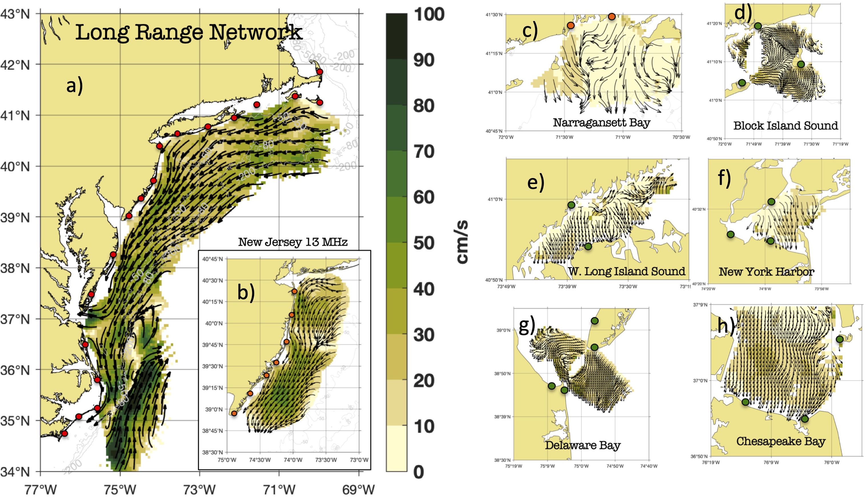
Figure 1 Map of the MARACOOS HF Radar Network (A) 5 MHz network consisting of 18 stations (B) 13 MHz network consisting of 7 stations in New Jersey (C) 16 MHz network covering Narragansett Bay with 2 stations and 25 MHz network consisting of 15 stations distributed over 5 domains (D) Block Island Sound (E) Western Long Island Sound (F) New York Harbor (G) Delaware Bay and (H) Chesapeake Bay.

In 2016, U.S. IOOS certified MARACOOS as a full member of the national IOOS system. Being certified as a Regional Information Coordination Entity (RICE) places it under the authority of the Integrated Coastal and Ocean Observation System Act of 2009 (ICOOS Act). Certification of IOOS Regional Associations is a detailed review and assessment process and provides NOAA and its interagency partners a means to verify a Regional Association’s organizational and operational practices meet recognized and established standards set by NOAA. This includes all aspects of data collection and management. The IOOS certification process does not follow an international standard; however there is a rigorous process for becoming a certified Regional Information Coordination Entity that is documented on the IOOS website https://ioos.noaa.gov/about/governance-and-management/certification/. As part of the certification process, each RICE is required to describe its data quality control procedures for the data it collects and distributes. All data shall be quality controlled and procedures shall be employed following quality assurance of real-time ocean data (QARTOD). In 2021, MARACOOS was recertified for another five years.

This manuscript describes an HF radar processing methodology, representing the combination of a suite of widely used QA/QC practices that are implemented in an efficient way through the use of automated diagnostic plots and community quality control software. The further development of HFR community software packages allows for the standardization of these practices on a wider scale. These methodologies have been conceptualized, tested and hardened over the past 20 years while operating High Frequency radar systems in the Mid Atlantic of the United States. Quality control practices are constantly evolving and we provide here a summary of at present QA/QC methods that we hope to update regularly which in itself is a best practice (Pearlman et al., 2019). Currently the MARACOOS team meets once a week to discuss existing data quality and develop new methods for improving data quality. We submit a description of our practices to the oceanographic community for consideration as a “Best Practice”. Section 2 describes the data flow from radar to total vector map and the associated best practices and QA/QC methods applied at each level. Section 3 discusses how the quality control techniques impact the comparison of HFR data with ADCP and drifter data. Section 4 is a discussion of QC flags, best practices and the challenges faced by the radar network. Section 5 provides concluding remarks.

2 Methods

An overview of the HFR data processing is provided in Figure 2. All but two of the radars in MARACOOS are the SeaSonde model manufactured by CODAR Ocean Sensors and the processing descriptions in this paper apply to those systems. The SeaSonde utilizes a three-element receive antenna mounted on a single post. The receive antenna consists of two directionally dependent cross-loops and a single omnidirectional monopole. The SeaSonde utilizes frequency modulation to determine range and direction finding for bearing (Barrick & Lipa, 1997; Kohut & Glenn, 2003). Radials are generated at the station and sent to data assembly centers (DAC) which combine the radial data into a total surface current map on a regular grid. These gridded total vectors are made available for applications such as the assimilation into the statistical and dynamic models operated in the region (Wilkin & Hunter, 2013) and the calculation of NOAA tidal current predictions.

Figure 2

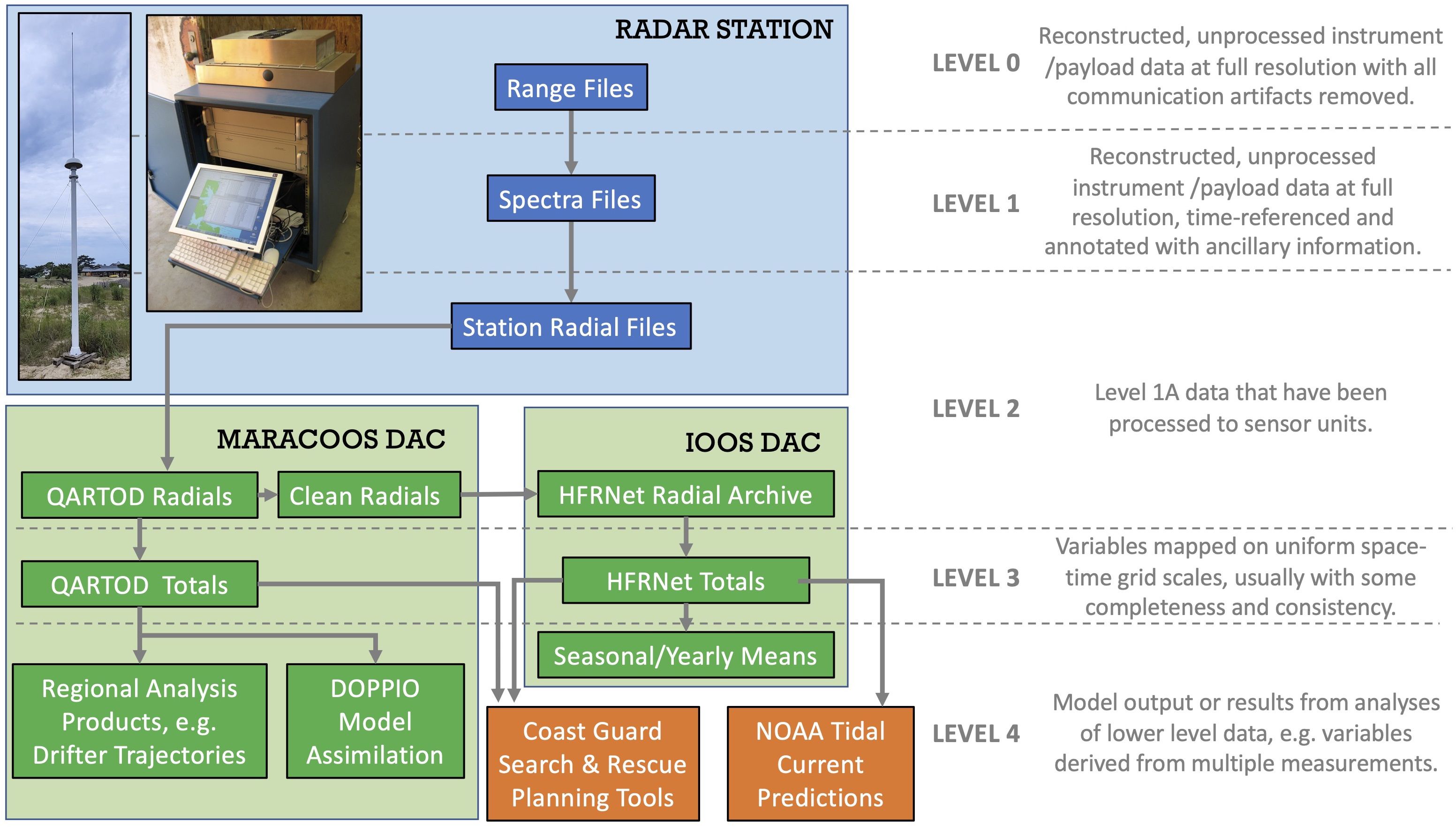
Figure 2 Flow chart of the HF radar processing chain from Level 0 data (quality assurance and range series files) to Level 4 data (derived products). The blue region indicates processing at the radar station, green for processing at the data assembly center and orange for usage by external stakeholders.

The components of the HF radar data processing chain have been mapped onto the data levels presented in the NASA Earth Science Handbook (Parkinson et al., 2006). There are a total of 5 layers with Level 0 representing the unprocessed instrument data at full resolution and Level 4 signifying derived products. We declared that the radial velocity data from the radar should correlate with Level 2 data, which are derived geophysical variables. Level 3 represents data on a uniform space-time grid and corresponds with the total vector currents. Level 0 to 2 data is processed at the individual radar stations while processing levels 3 and 4 take place at the DAC or at locations of external data users. This HFR mapping framework was first proposed at an Marine Technology Society OCEANS Conference (Roarty et al., 2016b) and has now been adopted by others in the community (Mantovani et al., 2020). Mapping the HF radar processing chain onto a common template with other remote sensing methods may identify ways to leverage QA/QC methods or practices that have been developed in other communities of practice (Kerfoot et al., 2016; Smith et al., 2017).

2.1 Level 0

We associate Level 0 data with any quality assurance methods that are conducted at the radar station. These include proper site setup and maintenance, remote monitoring, on-site inspections, and calibration with antenna pattern measurements. Technical expertise for operations and maintenance is shared during regular conference calls with operators in the region and spare hardware resources are shared amongst partners.

Some of the ancillary equipment we deploy at the station to ensure proper operation of the hardware includes an enclosure for the radar equipment, an air conditioning unit to remove humidity from the enclosure and keep radar equipment cool in the summer months, a lightning protection kit for the antennas, additional station lightning protection to minimize damage from a direct lighting strike, an uninterruptible power supply (UPS) to condition the incoming power and keep the station operating for short periods of time (under one hour) if power is lost at the station, a remote power switch that allows us to remotely cycle power to any component of the radar system and lastly a router to manage the communication to the station and communicate with the UPS and Web Power Switch. These supporting assets are similar to hardware accessories used by other operators (Mantovani et al., 2020). The stations utilized phone lines for communication early on, but these have been completely replaced with cellular modems.

We remotely inspect the radar station once a week by remotely logging into the station computer or viewing the hardware and radial diagnostic data through the stations’ Radial Web Server to perform an inspection following guidance from the manufacturer (Barrick et al., 2011) and the HF radar community (Cook et al., 2008). The technicians visit the stations at least once every 6 months to physically inspect the radar hardware and ancillary equipment.

The pattern of the receive antenna should be re-measured once a year or if data quality degrades (Kohut & Glenn, 2003; Laws et al., 2010). An antenna pattern is measured through a variety of methods: walking, boat, drone or AIS (Evans et al., 2015; Whelan et al., 2018). MARACOOS has implemented a real-time metric that checks for significant changes in measured pattern radial distributions over time based on a method developed by CODAR Ocean Sensors. It compares the distribution of the last five days of radial maps to a reference distribution using five days of maps generated after the most recent measured pattern was installed on the site using a Kullback–Leibler divergence index (KLDI) (Figure 3). This index is a statistical measurement that quantifies the difference between one probability distribution and a reference probability distribution, with higher values representing greater differences. Time series plots of the KLDI metric for each station are updated daily and posted online¹. KLDI values that increase and remain above a certain threshold indicate that a station’s measured pattern is no longer working well. If the metric remains above 0.1 for more than a week, a new antenna pattern is requested.

Figure 3

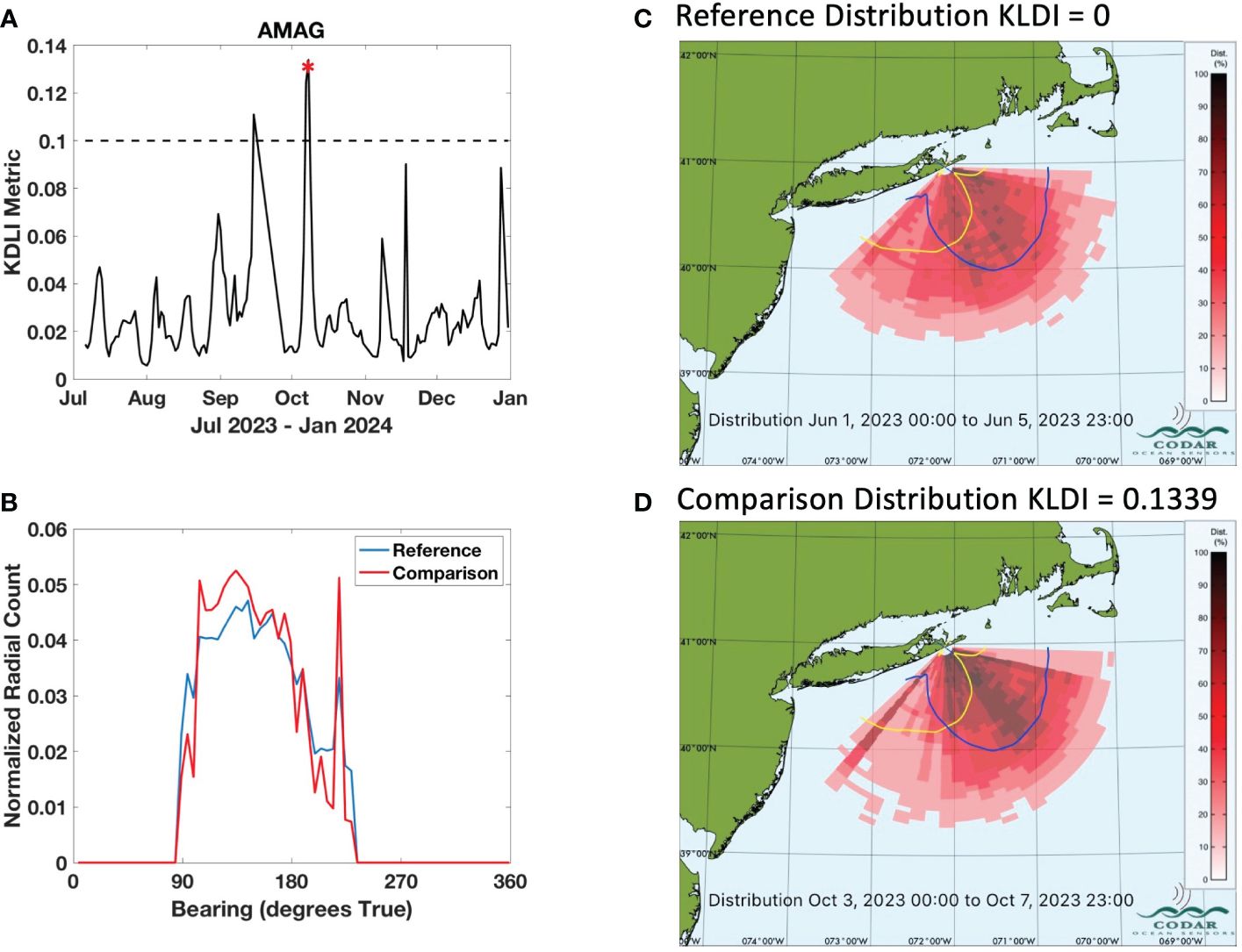
Figure 3 (A) Time series plot of the KLDI metric for the Amagansett, NY (AMAG) radar station (black line) and a warning threshold indicating an potentially invalid pattern (black dashed line) (B) Normalized radial distributions used to calculate the KLDI metric for the reference time period June 1-5, 2023 (blue line) and a later time period October 3-7, 2023 (red line) (C) Radial distribution for reference time period June 1-5, 2023 (red colormap) along with the antenna pattern for the radar (yellow and blue curves) (D) Radial distribution for later time period October 3-7, 2023 along with the antenna pattern for the radar (yellow and blue curves).

2.2 Level 1 – spectra

Level 1 data focuses on the step of generating velocity spectra from the radar. The settings for spectra collection for each of the frequencies are provided in Table 1. The relevant first-order scatter from the sea (Bragg echo) needs to be correctly extracted from the spectra for further processing into radial vectors. Rodriguez-Alegre (2022) presents a thorough description and explanation of the first order identification algorithms. We currently use the SeaSonde software to delineate the first order region of the spectra. Alternative methods (Kirincich, 2017; Rodriguez-Alegre, 2022) utilize image processing techniques and machine learning to draw this boundary and we are evaluating the impact of this new methodology. If a more efficient methodology for extracting the first order Bragg region becomes available, radial maps can be reprocessed using spectra which are archived at each operator’s institution.

Table 1

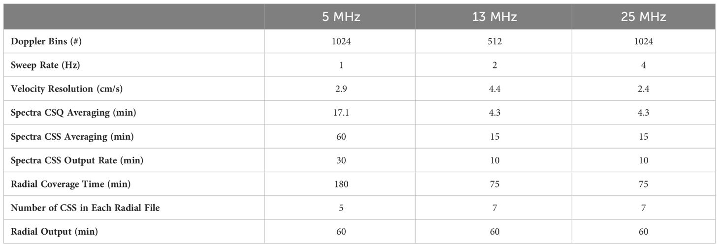
Table 1 SeaSonde Doppler, spectra and radial vector file processing parameters for each of the three frequencies operated within MARACOOS.

Each operator makes a monthly inspection of the first order delineation in the self-spectra to see if any of the processing parameters need to be adjusted to better capture the Bragg echo. The shape of the Bragg echo varies based upon the type of current that is being measured. Figure 4 shows the self-spectra (CSS) from the three frequencies operated within the Mid Atlantic, including a 5 MHz station in Loveladies, NJ (LOVE), a 5 MHz station in Buxton, NC (HATY), a 13 MHz system located in Seaside Park, NJ (SPRK) and a 25 MHz station in Staten Island, NY (SILD). In these plots, the x-axis represents radial velocity (cm/s), the y-axis represents range (km) and the color indicates echo signal strength (dB). The first order Bragg echoes appear as the flame-like shapes with the strongest signals and the white lines are delineations of that first order echo by the SeaSonde software. Second order echoes are not always present, but they may appear on either side of first order. In Figure 4C, second order peaks are visible in the positive radial velocity side to the right of the first order Bragg. For a majority of the stations within the Mid Atlantic the shape of the first order echo is a simple rectangle (Figures 4A, C). However, when the flow field is strong and variable as in the case of the Gulf Stream currents offshore of HATY or the water exiting NY Harbor measured by SILD, the shapes can be complex and it may be challenging to delineate the first order region for radial current processing.

Figure 4

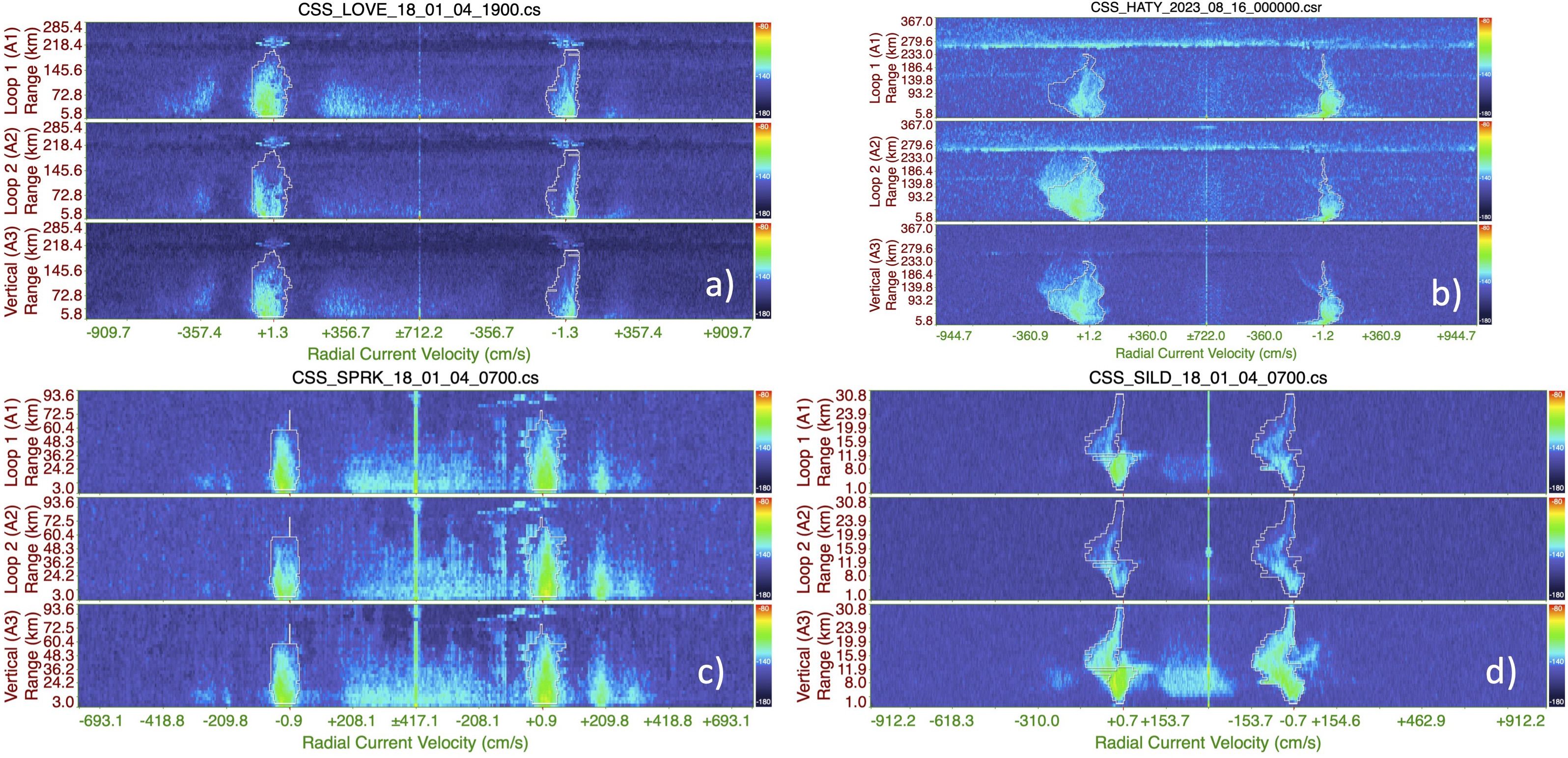
Figure 4 Spectra files from (A) 5 MHz system that covers the shelf (B) 5 MHz system that covers the Gulf Stream (C) 13 MHz system that covers the shelf (D) 25 MHz system that covers the entrance to NY Harbor with strong tidal currents.

2.3 Level 2 – radials

Generation of radial files involves several processing steps that take place at the radar station. The first order spectra from Level 1 are passed to the direction-finding algorithm MUSIC, which uses an ideal or measured antenna pattern to determine the bearings associated with first order reflections so that radial speeds can be properly mapped (Lipa et al., 2006; Cook et al., 2007). MUSIC processing produces radial metric files, which are then processed to short term radial files. The short-term radial files are concatenated and the median velocity in each range and angular bin is chosen as the velocity for the merged hourly file. The software is configured to require at least two vectors in the short-term radial ensemble in order to output a velocity measurement in the hourly file. The requirement of two vectors minimizes the error in the velocity measurement (Kohut et al., 2006b). On each radar station, a custom angular segment filter (named AngSeg_XXXX.txt located in the station configuration folder where XXXX is the four-letter site code for the station) is applied to the merged radial file. This filter is used to flag radial vectors that are placed in unreasonable locations, i.e. over land or behind islands. This also limits the angular coverage of the radial file to flag radial vectors derived from radar signals that would have excessive land paths back to the receive antenna. Radial files generated with a measured antenna pattern are referred to as measured radials and those generated with an assumed ideal antenna pattern are referred to as ideal radials. For a further description of the SeaSonde analysis procedure see (Lipa et al., 2006; de Paolo & Terrill, 2007; Kirincich et al., 2012).

The radial files are transferred back to the regional DAC at Rutgers once an hour via rsync over secure shell. As soon as a radial file arrives, a watchdog program initiates software that performs QC on that file. The radials are quality controlled according to the most recent version of the Quality Assurance/Quality Control of Real-Time Oceanographic Data (QARTOD) for High Frequency Radar surface current data (Bushnell & Worthington, 2022). The software used to perform the QARTOD tests is found in HFRadarPy (Smith et al., 2022), a Python package designed for exploration, cleaning and manipulation of HFR data. The quality tests applied to the radial data include file syntax, maximum speed, valid location, radial count and spatial median. All radial vectors are marked according to the QARTOD flagging definitions of pass (1), not evaluated (2), suspect (3) or fail (4) (Gouldman et al., 2017).

Primary and secondary flags are written to the radial file based on the QARTOD tests. The primary flag is meant to provide users with an overall assessment of data quality and can be used to quickly filter out bad data. The secondary flags are the results of individual QC tests. The primary flag for a radial vector is set to a fail code (4) if any of the specified secondary flags has a fail code. Radials that fail are excluded from the total vector calculation. The new radial QC file retains the same name as the original radial file and keeps all of the information from the original file. QC test metadata is added to the file header and the flag code results for each test are appended to the CODAR main data table in separate data columns. When an entire file fails based on a test such as syntax or radial count, fail flags are set for every vector in the file (Updyke et al., 2021). Lastly a cleaned version of the radial file is created, which only contains data that has passed quality control (primary flag not equal to 4). This file is then passed to the IOOS surface current data assembly center (HFRNet) for total vector processing.

Monitoring practices at the MARACOOS DAC help streamline the processing as well as alert operators to any problems. The radial metadata are inserted into a Mongo database to allow for quick retrieval of station diagnostic information and to monitor which sites in the network have contributed a radial file for a particular hour. The latest radial information from each of the stations can be found on the Radial Diagnostic Dashboard² hosted on the Rutgers University website. The Dashboard displays the timestamp of the latest radial file, the radial vector count of the file, transmit frequency and preferred radial type (ideal or measured) that will be used in the total processing. If the most recent radial data is older than 12 hours the background color of the radial station changes to alert the technicians to the deficiency. An outage report is automatically created and the technicians also receive an email alert. Information for each outage, including duration and cause, is saved in the database and displayed online.

In addition to monitoring for data gaps, the DAC creates several automated plots that operators use to evaluate data quality. Figure 5A shows a plot of a typical radial file. Radial maps are made with the blue/red colormap where blue indicates vectors that are travelling towards the radar and red vectors indicating currents that are travelling away from the radar, consistent with redshift and blueshift from electromagnetic Doppler phenomenon. This two-color map aids in quick identification of areas that have contrasting directions of flow, which may signify flow dynamics of particular interest or indicate vectors that have potential data quality issues. We utilize the 25-hour mean radial map (Figure 5B) and a weekly plot of average radial velocity and radial vector count (Figure 6) as quick diagnostics for station health. These diagnostics are similar to those of previous researchers (Kim, 2015). Abnormally low radial counts are caused by a low radar signal to noise ratio (SNR) and the reason for the low SNR must be investigated. When low SNR is due to equipment failure or high background noise levels, the radials are likely to be of poor quality. Other initial QC checks include those for spatial consistency within each station map and between neighboring station maps. Figure 5A shows smooth transitions in radial flow and no spatial outliers in speed or direction. The southern section of this map shows radial flow directed away from the antenna. If for example, a single bearing in that section included vectors directed towards the antenna, this would be a spatial inconsistency of concern. The radial maps in Figure 5 indicate a general flow towards the southwest; however, if nearby radar stations all indicated flow to the north, this would indicate a quality issue. The current flow must be physically reasonable. Another quick check of this in our region is to see that the periodicity of the average radial velocity time series (Figure 6) is visually consistent with the ebb and flow of a semi-diurnal tide. We have also found that a consistent average radial bearing (Roarty et al., 2012b) is an indication of a properly operating station and if this measurement has a step change or becomes erratic then that is an indication of a failure somewhere within the system. Whenever inconsistencies are found, the data are considered suspect and the operator will update a configuration file in the database to either remove the radial station from the total vector processing or change its preferred pattern type for processing. The operator will then begin an inspection of the system to identify any problems.

Figure 5

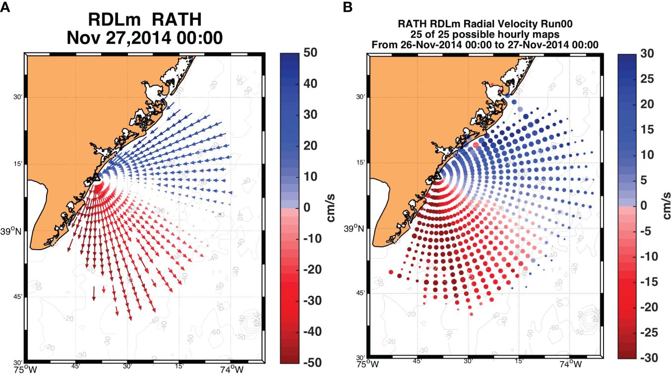
Figure 5 (A) Example of a radial map for a 13 MHz station. (B) 25-hour mean of radial velocities. The average velocity is represented by the color and the standard deviation by the size of the dot.

Figure 6

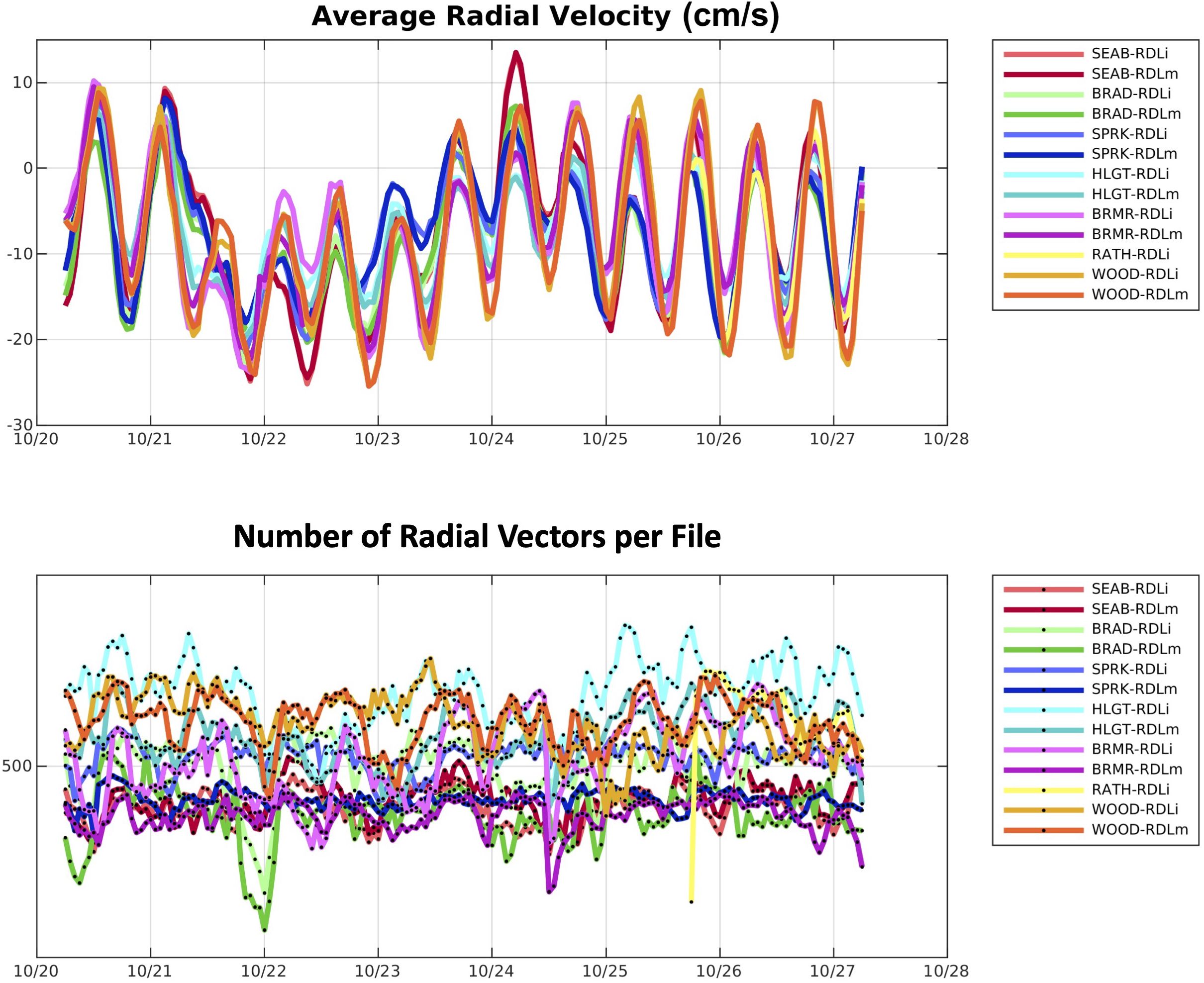
Figure 6 One week plot of average radial velocity (top) and radial vector count (bottom) for the ideal and measured radial files of the 13 MHz radar network.

2.4 Level 3 – totals

The processing of total vectors runs once an hour to combine the radial velocity measurements into an evenly gridded total surface current product. When the total generation script runs it checks the Mongo database to see what radials are available at that time. The software also checks back 168 hours (1 week) to see if any radials were late in arriving at the DAC and will reprocess the total file if a radial file is now present. The MATLAB community toolbox HFRProgs (available on GitHub) is used to generate the total vector files. The radial vectors are screened so only vectors without fail codes in the primary flag are included in total vector generation. The configuration file within the database sets the pattern type (ideal or measured) to be used in the processing. The preferred radial type for total generation is measured; however, the ideal type may be used if the measured file is not available or found to be questionable.

The radial files are combined with two methods, unweighted least squares (UWLS) and optimal interpolation (OI), to produce two distinct total vector products. The configuration parameters for the UWLS and OI total surface current products are given in Table 2. In areas of good geometry and radial data coverage the algorithms are similar, however the OI outperformed the UWLS in the prediction of a surface drifter over 12 hours (Kohut et al., 2012). The surface drifter is the preferred instrument the Coast Guard uses for evaluation of surface currents during search and rescue missions (Allen, 1996) and the 12-hour threshold is the maximum length of drift scenario that would be used by the Coast Guard; therefore we chose the OI product as the one we would deliver to the Coast Guard and other stakeholders as the operational product.

Table 2

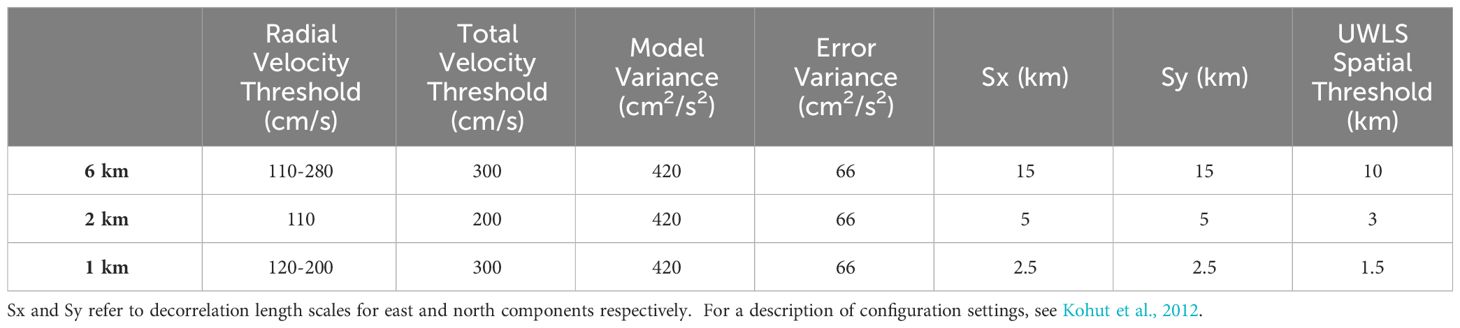
Table 2 Processing parameters and velocity thresholds for the unweighted least squares (UWLS) and optimal interpolation combining methods.

Currently, only radials from similar frequency and averaging parameters are combined to form total vector products within the region. The combining grids were provided by the US National HF Radar Network (Terrill et al., 2006). The radials from the 5 MHz radars are combined on a 6 km grid, the 13/16 MHz radials on a 2 km grid and 25 MHz radials on a 1 km grid. This is unlike the U.S. National Network that combines radials from multiple frequencies and processing configurations into its 6 km and 2 km products. It has been noted that radial velocity maps with higher spatial resolution would produce a bias in the total vector map if combined with radial files with lower spatial resolution (Kim et al., 2011), so the decision was made to only generate totals with radials with similar averaging and processing schemes. Also, the temporal averaging differs for the frequencies that are operated in the region, 180 minutes for the 5 MHz radars and 75 minutes for the 13 and 25 MHz radars. Operators have experimented with shorter averaging intervals for the 5 MHz (Roarty et al., 2013a) and 25 MHz (Chant et al., 2008) but have not implemented them operationally.

The total vector files are quality controlled according to the HFR QARTOD manual (Bushnell & Worthington, 2022). The total vector data are subject to the data density (a minimum of three radial velocities must be sourced from at least two radar stations in order to compute a total velocity vector), maximum speed (total velocities > 300 cm/s are flagged as failing), valid location and velocity uncertainty tests. The u component (eastward) and v component (northward) velocity uncertainties are normalized uncertainties that are calculated as part of the optimal interpolation algorithm. A value of 0 is good and a value of 1 is poor. In the Mid-Atlantic, a previous study by Kohut et al., 2012 showed that a threshold value of 0.6 improved data quality while preserving good data coverage in the total vector maps.

The total vector data are saved in MATLAB (.mat) files in the HFRProgs TUV data structure as well as climate and forecast (CF) compliant NetCDF files. The quality control flags are stored in the MATLAB files as additional fields of the TUV structured array. In the NetCDF files, the flags are represented as additional variables and those variables include attributes that describe the flags and the tests. The radial and total vector files are served to the oceanographic community and public through several methods. The data files can be accessed and downloaded through the Thematic Real-time Environmental Distributed Data Services (THREDDS)³ (Unidata, 2017) interface or via ERDDAP⁴ (Simons, 2017). The surface current maps can be visualized through the MARACOOS data portal OceansMap available at http://oceansmap.maracoos.org, the National HF-Radar Network https://cordc.ucsd.edu/projects/hfrnet/ or the National Data Buoy Center https://hfradar.ndbc.noaa.gov

The hourly gridded total maps are the data product of interest for most applications at this time. The maps are reviewed to look for errant vectors. If a total map has suspect vectors, the radial files in the vicinity of the suspect area are plotted. If a particular radial file/station is found to have errant vectors, the cause of the error is investigated and adjustments are made to the processing to eliminate the error in future maps.

2.5 Level 4 – derived products

Level 4 data is treated as analyses from lower Level 3 data i.e. variables derived from multiple measurements. The types of products that are generated include daily, seasonal and annual means of the Mid Atlantic surface currents (Gong et al., 2010; Roarty et al., 2020), virtual Lagrangian drifter trajectories (Roarty et al., 2016a; Roarty et al., 2018) and Eulerian velocity time series at any point in the field of coverage. For daily, monthly or yearly maps of the surface currents we typically require 50% temporal coverage and the OI normalized velocity uncertainty to be below 0.6 (Kohut et al., 2012) at a grid point in order for a vector to be displayed.

2.6 Network performance metric

The MARACOOS 6 km surface current product has been operational with the Coast Guard for search and rescue since May 4, 2009. A requirement from the Coast Guard for this new data product was consistent temporal coverage and spatial coverage over a majority of the Mid Atlantic. Therefore, a spatial and temporal coverage metric was developed to gauge network performance which in turn helped guide the efforts of the technical staff operating the network. The goal is to achieve 80% temporal coverage over 80% of the Mid Atlantic over a six-month period, which is the reporting interval for MARACOOS. The spatial coverage entailed the 6 km grid beyond the 15 m isobath within 150 km of the coast between latitude 35° to the south and 42° to the north. The 15 m isobath was chosen as the inward boundary because the measurements from the 5 MHz radars will include a bias in water depths shallower than this threshold. The radio wavelength for the 5 MHz radars is 60 m and these radio waves scatter off ocean wavelengths of 30 m. From linear wave theory, wave speed is altered when d/λ<0.5, where d is the water depth and λ is the ocean wave length. The 150 km outer boundary was chosen as the minimum nighttime range of the 5 MHz radars.

Figure 7 presents the network coverage from June 2011 to February 2022. This is a marked improvement over the network performance that was first published in 2012 (Roarty et al., 2012b). MARACOOS was able to exceed the 80/80 goal for nearly all progress, even during the December 2012 period just after Hurricane Sandy badly damaged the network (Malakoff, 2012). The four failures to meet the goal were due a combination of factors. The coverage of the network has degraded recently as the funding has not kept up with inflation and the equipment continues to age with many of the radars older than 20 years. The COVID-19 pandemic also impacted technician response time and hardware repair turnaround times. One of the biggest contributing factors to missing the goal was due to the locations of the particular stations that experienced extended outages. In the northern section of the region, adjacent sites had extended outages at the same time. Whenever adjacent stations are offline, this has a much greater negative impact on the spatial coverage of the total map product. In areas where radars are more densely spaced along the coast, such as New Jersey, losing one station will not create as much of a data gap since overlapping radials from the neighboring stations are still available to generate totals for much of the area. An extended outage for the Cedar Island station on the Eastern Shore of Virginia also created a large spatial gap as there are not many suitable powered locations for radar stations along that section of coastline and the neighboring stations are far enough apart that overlapping radial coverage is limited.

Figure 7

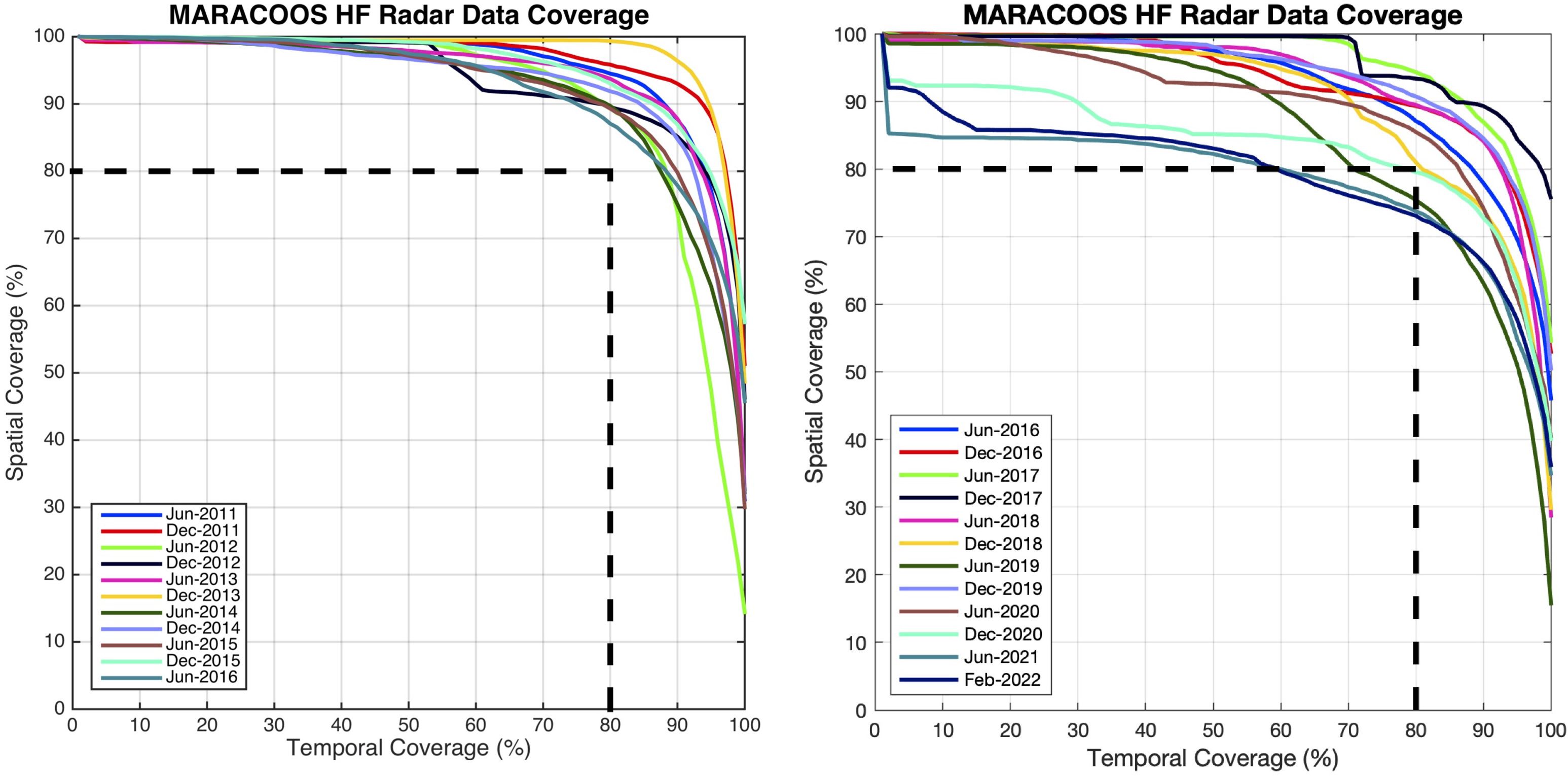
Figure 7 Total surface current performance metric for the 6 km product. The x-axis represents temporal coverage and the y-axis represents spatial coverage. Each of the colored solid lines represent the the network performance for the 6-month progress periods within MARACOOS. The dashed black line at 80/80 is the goal for network performance as established with the Coast Guard Office of Search and Rescue. The left panel represents the progress periods from 2011-2016 and the right panel shows network coverage from 2016-2022.

3 Results

This section first describes two previous studies that were performed in 2016 to quantify the impact of these quality control concepts. We discuss the difficulties in assessing the value of QC with these approaches and then report on recent analysis that seeks to better characterize the value from a wider perspective. In the 2016 studies, HFR data (with and without additional radial QC tests applied), were compared to in-situ measurements of surface currents from an Acoustic Doppler Current Profiler (ADCP) and to surface drifter data provided by the Coast Guard Office of Search and Rescue.

A four-month data set of HF radar surface currents from the New York Bight Midshelf Front Experiment (NYBMFE) (Kohut et al., 2012; Ullman et al., 2012) was compared to measurements taken from the closest surface bin of an ADCP. We then quantified the impact of using additional radial QC tests on the HFR data before making the comparison. We also assessed the difference between using measured pattern radials and using ideal pattern radials in the comparison. Preliminary results were previously published in conference proceedings (Roarty et al., 2016b). When the NYBMFE was conducted, only a limited number of radial QC tests were in place including a syntax test, over-water test, and a global range (maximum velocity) test. Three additional radial tests were used in reprocessing for this experiment: 1) local range (maximum velocity), which tests whether a velocity measurement falls outside a pre-defined range 2) stuck sensor, which tests if the velocity measurement has repeated occurrences of the same value and 3) temporal gradient, which tests if changes between successive measurements fall outside a predetermined range.

First, appropriate thresholds needed to be defined for each of the tests. The local range (maximum velocity) test thresholds were selected after reviewing one year of radial velocity measurements at different locations. Greater flow speeds and larger variability are associated with the Gulf Stream and the currents in New York Harbor, while shelf currents are slower and less variable. A local range threshold of 150 cm/s was chosen for stations observing shelf waters not located near the Gulf Stream and a higher threshold of 250 cm/s was set for stations observing strong tidal currents in estuaries or those measuring the Gulf Stream. Note that the maximum velocity thresholds reported in the methods section above were developed later and not in use when this analysis took place.

The stuck sensor test checks for repeating values in the time series. If successive measurements do not exceed the resolution of the measurement for a certain amount of time, the values are considered “stuck” and will fail the QC test. The resolution defined for the purpose of this test was 0.01 cm/s. The time threshold was set to three hours. The stuck sensor test identified gaps in velocity solutions at a particular range and bearing cell. The radar processing picks the median velocity from the ensemble of radial short files. If there are missing solutions over an averaging period then the median velocity repeats and is flagged by the stuck sensor test. The temporal gradient threshold was established using the ADCP record. The ADCP surface bin was rotated into a radial and cross radial coordinate system relative to the radar station at Wildwood, NJ (WILD). The temporal derivative over one hour in the radial direction was calculated for the four-month velocity record. The median of that record was -1.15*10^-4 cm/s² and mean was -2.5*10^-8 cm/s², both close to zero. The 95^th percentile value of 0.005 cm/s², was chosen as the gradient threshold. This equates to a velocity change of 18 cm/s over an hour and any radial velocity with a temporal derivative greater than this threshold was flagged as failing the test.

The thresholds explained above were used to flag the HF radar measurements. MARACOOS follows the flagging scheme established by the Quality Assurance of Real-Time Oceanographic Data (QARTOD) (Gouldman et al., 2017) The radial velocities with fail flags were then removed from the record and the remaining data was compared to the full ADCP record. Then eight combinations of the three tests were utilized to determine if the comparison between the radial velocity from the WILD radar station closest to the ADCP would be improved. Test 1 kept all the HFR data while Test 8 removed any radar data that failed the local range, stuck sensor or temporal gradient test. The statistics for the comparison between the ADCP and the ideal and measured radials are given in Table 3. In this experiment, the use of ideal or measured radial files was comparable. In the ideal radial comparison, there was a 4% improvement in root mean square difference (RMSD) for test 8, which utilized all three quality control tests; however, 9% of the data was removed. For the measured radial comparison, both correlation and RMSD decreased with the use of all three quality control tests. There was no discernible change in the correlation between the HFR and ADCP data through the use of the QC tests.

Table 3

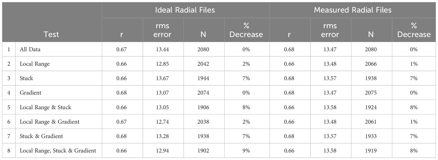
Table 3 Correlation (r), root mean square error (rms error cm/s), number of samples (N) and percentage decrease of the original data record based on 8 combinations of quality control tests for the WILD ideal (left) and measured (right) radial files.

Recognizing the limited scope of the first study as a comparison at a single location for one radar station, the next test of the quality control concepts used surface drifters so that given the Lagrangian nature of the drifter current measurements, larger areas of radar coverage for multiple stations could be tested. The analysis presented here was conducted as part of a validation experiment of the radar network in conjunction with the Coast Guard Office of Search and Rescue. Three clusters of Coast Guard surface drifters (Allen, 1996) were released: one cluster along the 30 m isobath in the northern area of the 5 MHz network, one along the 70 m isobath in the northern area of the 5 MHz network and one along the 30 m isobath in the central region of the 5 and 13 MHz network (Roarty et al., 2018). The average surface drift is towards the southwest so the hope was that the drifters deployed in the northern region of the network would drift through the majority of the network coverage. The drifters remained in the northern and central region for the experiment so the full network wasn’t tested near Virginia and North Carolina, but the drifters endured for an average of 36 days providing a robust data set.

The drifters reported position data every 30 minutes. The drifter data were interplated to hourly intervals to match the temporal sampling of the radar data. If a drifter passed through the coverage area of one of the radar stations, the velocity of the drifter was rotated into a radial velocity relative to the particular radar station. Then the closest radial velocity from the radar station was paired with the radial velocity of the drifter for comparison. An example of this comparison is shown in Figure 8 where drifter 43346 was compared to the radial velocity from the radar station at Brant Beach, NJ (BRNT). This comparison was repeated for each of the seven drifters against eleven radar stations. The radial velocity correlation and root mean square error (RMSE) between the drifter and radar station are shown in Table 4. Seven of the stations showed high correlation with the surface drifters. The radar stations that showed low correlation (Martha’s Vineyard, MVCO; Nantucket, NANT and Misquamicut, MISQ) were due to hardware problems at the stations that had not been repaired yet. Three stations (AMAG, MRCH and BLCK) displayed low correlation with the same drifter 43104 so there may have been errors in the position reporting of that particular drifter.

Table 4

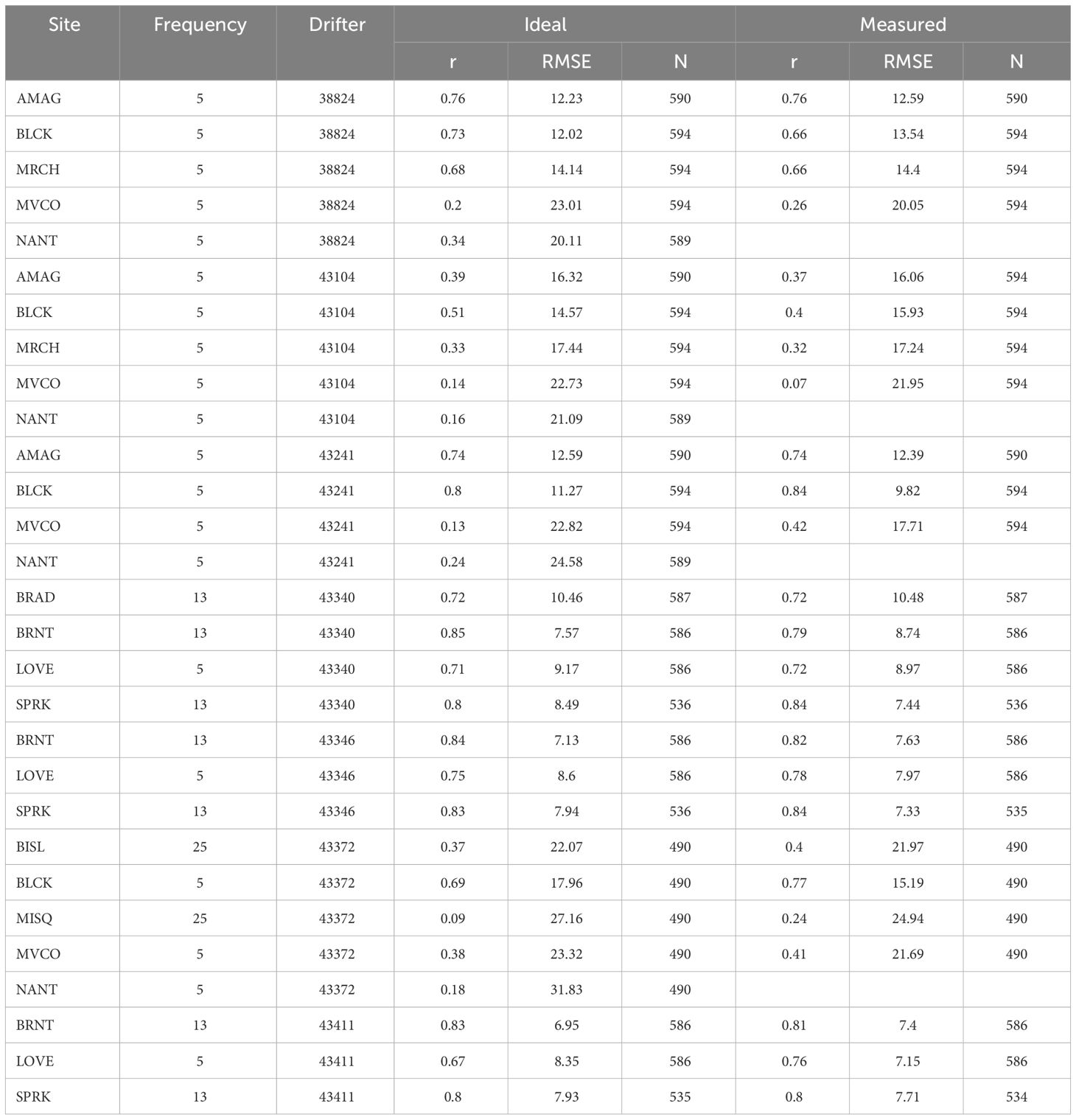
Table 4 Correlation (r), root mean square error (RMSE, cm/s) and number of data points (N) between radar station radial data (ideal and measured) and surface drifter.

Figure 8

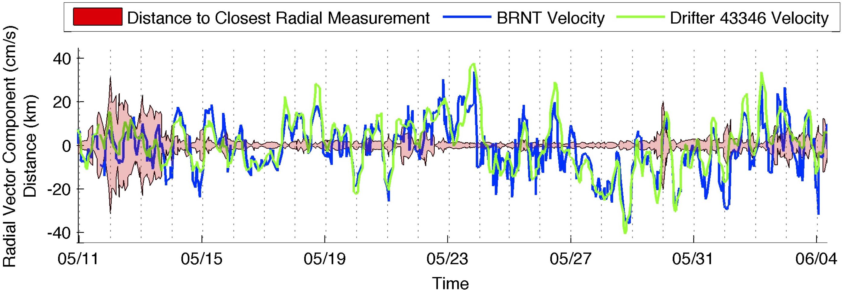
Figure 8 Radial velocity of drifter 43346 (green) relative to radial velocity of radar station at Brant Beach, NJ (BRNT) (blue). The distance between the drifter and the nearest radial velocity at a particular instance of time is shown as the shaded red region.

A subsequent analysis compared the skill of predicting drifter tracks with two datasets of HFR surface current maps, real-time and reprocessed, from the year 2017. The results quantify the impact of the use of additional QA/QC in the reprocessed data. The real-time dataset for radials included 1) operator review of hardware and radial diagnostic plots, 2) operator review of radial maps and radial distributions, 3) operator evaluation of which radial type to use in totals (ideal or measured pattern), 4) removal of data over a set maximum speed at the spectra level using manufacturer software, 5) flagging of invalid locations using manufacturer software and 6) radial file syntax requirements. Additional QA/QC for reprocessed maps included 1) a systematic review of data and diagnostics by the MARACOOS QC group to remove questionable data, 2) reprocessing radials from spectra if more suitable calibration patterns were available, 3) applying radial metric QC (Haines et al., 2017) to North Carolina radar stations, 4) applying QARTOD radial count and spatial median radial QC tests, which were not in use in real-time data in 2017 and 5) re-calculating totals with radials that did not fail any of the QC tests. Table 5 compares the performance of each dataset using a Lagrangian skill score (Liu & Weisberg, 2011). Skill at predicting a drifter track was improved significantly by using the reprocessing dataset for drifter 65247790 near the Outer Banks. The skill for drifter 63804280 was higher using the real-time dataset; however, it is worth noting that this case had an extremely low skill score count. For other drifters, skills were the same or slightly improved. These results provide comparisons throughout the Mid-Atlantic although the comparisons are only available for the duration of time that the drifter is located within the radar coverage. Each skill score represents a comparison over six hours so based on the number of scores per drifter, the minimum duration of a comparison was 12 hours (2 scores for drifter 63804280) and the maximum was 384 hours (64 scores for drifter 63783850).

Table 5

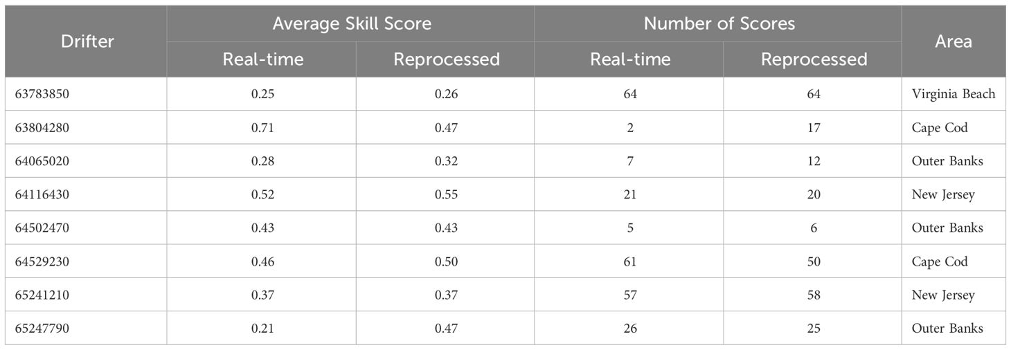
Table 5 HFR skill at predicting drifter tracks of Coast Guard drifters deployed in the Mid Atlantic in 2017.

We have used comparisons of HFR data with currents measured by other instruments to evaluate the effectiveness of quality control; however, this is not the only way to assess benefits of QA/QC. Poor quality is sometimes evident and can be identified even when a separate verification data set is not available. One source of measurement error is the processing of spectra that is not sea echo and an example of this is the processing of ionospheric reflections that are recorded in the spectra. All the radars operate with the manufacturer supplied filter that is applied to each Doppler spectra, where interference that is detected is removed from further processing. However, the existing filter does not catch all ionospheric interference. Ionospheric interference is characterized by increased signal strength stretching across the Doppler cells but confined to a few range bins. Those reflections in the radar data are of interest to researchers who study the ionosphere (Kaeppler et al., 2022); however, this interference can lead to large velocity vectors being added to the radial maps, which in turn, cause errant patches of high velocity data in the total maps. Figure 9 shows an hourly map when the Duck, North Carolina (DUCK) radar station exhibiting ionospheric interference as the large red vectors and the same map where the ionospheric interference has been removed through the use of the spatial median test. Figure 10 shows the positive impact that flagging and removing these types of erroneous vectors can have on the surface current maps. The high velocity patch seen in the map on the left of the figure is caused by the noise being processed to radial vectors and that patch is removed when QC tests, including the spatial median test, are applied in the processing.

Figure 9

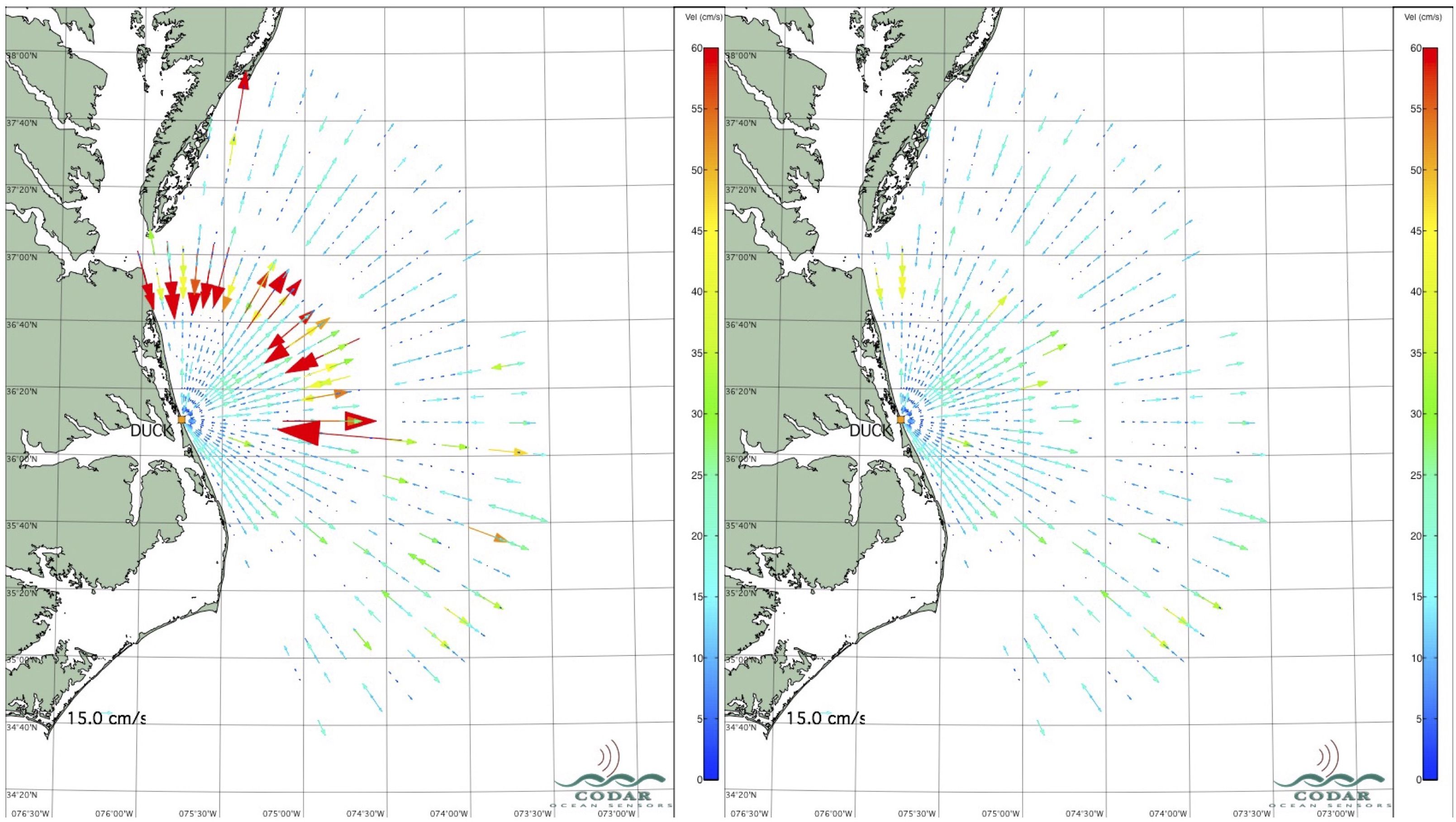
Figure 9 Map of radial files from the Duck, North Carolina radar station for November 9, 2016 23:00 UTC. Left panel: Map including erroneous high velocity radials caused by processing of ionospheric interference. Right panel: Map after applying a spatial median QC test to flag and remove spatial outliers.

4 Discussion

4.1 Utilizing flag information

The total count of flags for each of the individual radial tests (syntax, maximum velocity, valid location, radial count, spatial median, temporal gradient and stuck sensor) and the primary flag are plotted as a time series for the past week⁵. This online visualization allows the operators to detect any changes with respect to the radar operations by identifying time periods with high numbers of suspect or fail flags. The plots include two radial QC tests, temporal gradient and stuck sensor, that are staged for implementation at a future date. Tests under evaluation are added to the real-time processing, but the results are not considered when assigning a value to the primary flag; this means that those tests will not affect which radials are included in total vector calculations. However, the results of the tests are written to the QC version of the radial file and also plotted, which is useful because the plots of flag counts can be viewed to see if the new tests and test thresholds are working as expected. For example, if there are too many fail flags for a test at a certain site, a closer investigation of the performance of the test can be pursued and test thresholds could be adjusted for that station. When a new test is working well, it may be approved for inclusion in calculation of the primary flag.

4.2 QC challenges

The processing of ionospheric and other types of radio interference remains a significant QC challenge. The exact origin of interference might not be known, but it may still be visually apparent in a spectra colormap that other signals are being confused with sea echo (e.g. interference appearing as vertical or horizontal stripes covering wide areas of the spectra are also covering the first order sea echo). Radial vectors that contribute to unrealistic spatial patterns in the current maps can often be traced back to the locations in the spectra where interference intersected with the first order region. Flagging and removing these erroneous vectors from the maps can significantly improve data quality. In an application such as search and rescue planning, a high velocity patch such as that in Figure 10, would influence virtual drifter trajectories, carrying drifters further than they should travel in the time period for the search scenario and expanding the size of a search area. The QARTOD spatial median test occurs at the radial level; it can miss problems when there are few neighboring radials or a patch of erroneous data is large enough that the vectors in the middle of the patch pass the test. The development of additional QC measures to address interference at the spectra level would be an even better approach. QC is applied in the SeaSonde software to remove interference at the range and spectra level, but at the present time, it is only partially effective for some types of interference.

Figure 10

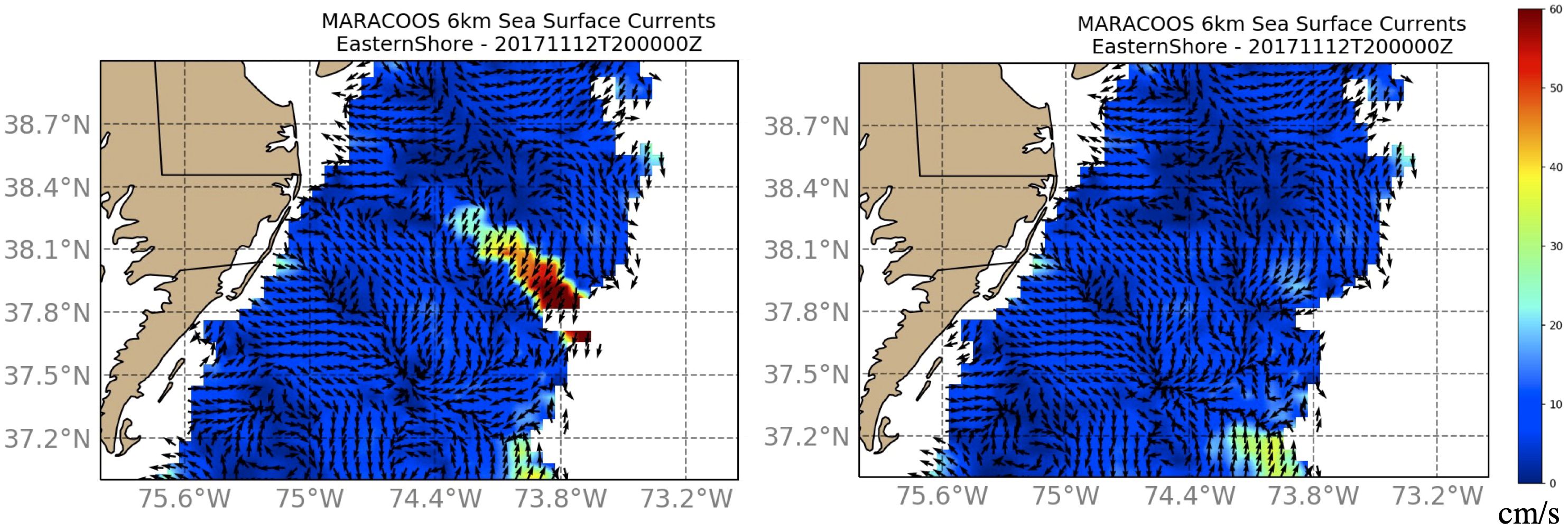
Figure 10 Surface current map for November 12, 2017 20:00 UTC. Left panel: Map calculated using real-time radials contaminated by ionospheric interference. Right panel: Map calculated with radials that had additional QC applied to flag and exclude spatial outliers from processing.

4.3 Best practices

The subject of quality control and best practices (Bushnell et al., 2019) has been a topic within the HF radar community for quite some time. The Radiowave Operators Working Group was formed in 2004 to help develop best practices for the burgeoning field of operational HFR remote sensing. The charter of ROWG aims to foster collaboration between new and experienced HFR operators, develop procedures governing HFR operations and provide recommendations to HFR stakeholders (data users, instrument manufacturers and program managers). The organization meets in person approximately every 18 months, maintains a listserv of approximately 140 members where members can communicate between meetings and supports a wiki www.rowg.org that serves as a knowledge repository for the operators. The operators also maintain several software repositories that are utilized in the management of HFR data and can be found at https://github.com/rowg. It should be noted that the HFR community was the first to update their QARTOD manual to provide community guidance and a roadmap for the ocean observing community.

HFR operators have also published several documents on best practices and quality assurance/quality control. Operators in California, USA developed the first best practices document on the deployment and maintenance of High Frequency radar stations (Cook et al., 2008). Operators in Europe have also made strides to document best practices and quality control (Rubio et al., 2017; Mantovani et al., 2020) as well as practitioners in Australia (Cosoli & Grcic, 2019). Both the Mantovani and Cosoli paper discuss best practices for both beam forming and direction finding radar systems while this paper focuses solely on the direction finding SeaSonde radar. Also, the Mantovani paper discusses the siting of new radar installations while this paper focuses on existing installations. One thing to note is that Australia utilizes UNESCO (Commission, I. O, 1993) flag codes while European HFR operators use the flag codes from the ARGO network (Wong et al., 2023). Both of these flagging conventions are slightly different from the QARTOD codes. The ability to manage these differing flagging schemes can be done through the use of a translation table (Bushnell et al., 2019). The unique aspect of our best practice manuscript is that we describe quality control tools that include dashboards and real-time automated plots that are implemented at the regional level.

4.4 Future QC work

Future QC plans include developing further use of radial metric QC (Haines et al., 2017) as well as implementing real-time baseline comparisons (Capodici et al., 2019) between stations and synthetic radial comparisons (Emery et al., 2022) for additional layers of quality control. Synthetic and baseline radial comparisons are a means of quantifying consistency with other HF radar measurements as a metric of quality. These are useful metrics given the unique spatial and temporal coverage of the HF radar, which complicates the evaluation of the data quality by means of comparison to data collected by other instruments, such as satellites, drifters or ADCPs.

This manuscript provides the most up to date summary of real-time delivery of surface currents from the Mid Atlantic High Frequency Radar Network. We are beginning to develop methods and the workflow to deliver a post-processed science quality product (Updyke et al., 2019; Smith et al., 2021) in addition to the real-time data stream. The quality control tests for reprocessed data may be applied somewhat differently from the tests for the real-time product. For example, the temporal QC test, such as gradient or stuck sensor, can be applied over time periods that extend further into the future as well as the past.

4.5 Operational challenges

There are two major challenges facing the network for continued success in the future: aging infrastructure and the development of offshore wind in the Mid Atlantic.

The radars that were first deployed in the region are reaching their end-of-life status. The MARACOOS radar community has designated the service life for radar chasses (receiver and transmitter) as 20 years. The exposed elements have shorter working life spans: 15 years for transmit antennas and 10 years for receive antennas which contain more sensitive electronics. Service life of the cables depends on the type of conduit and exposure, but is estimated at 10 years. Platform components like air conditioning units have a 10-year service life and computers are typically replaced every 5 years. The US network was envisioned to contain 321 radars (Harlan, 2015). At the current rate of expansion (26 stations added between 2017 and 2019, 9 per year), this will be completed in 2038. In order to complete the network by the end of the decade 25 new radars would need to be added to the network each year and 15 aging radars should be replaced each year.

The other challenge to the network is the 50 GW of offshore wind envisioned by the Mid Atlantic states. Land-based High Frequency (HF) Radars provide critically important observations of the coastal ocean that will be adversely affected by wind turbine interference (WTI). Pathways to mitigate the interference of turbines on HF radar observations exist for a small number of turbines; however, a greatly increased pace of research is required to understand how to minimize the complex interference patterns that will be caused by the large arrays of turbines planned for the U.S. outer continental shelf.

CODAR Ocean Sensors led a series of studies funded by the Bureau of Ocean Energy Management (BOEM) to understand the problem. The key findings of the first study (Trockel et al., 2018) are that the interference is caused by the amplitude modulation of the turbine’s radar cross section. The location of the interference is predictable and can be determined from the rotation rate of the turbine. The turbines interfere with HF radar processing in three ways: 1) raising the background noise level which affects the sea echo identification algorithm 2) changing the boundaries of the sea echo peaks by mischaracterizing turbine echoes as part of the sea echo and 3) affecting the bearing determination of radial current vectors by causing the turbine echoes to be convolved with the sea echo. The second BOEM study (Trockel et al., 2021) tested the mitigation strategies outlined in the first report. The overall result of the mitigation strategies led to a reduction of 86% of WTI in the first order region of SeaSonde spectra collected from a 5 MHz radar for a single month (March 2021). To assess the full impact of WTI on the HF radar enterprise, additional frequencies and longer evaluation periods will be needed.

The HF radar community self-organized to identify a roadmap for the next five years to tackle this problem (Kirincich et al., 2019). This led to the NOAA IOOS funded program (2020-2024) to advance the WTI mitigation from research into regular operations via a coordinated set of system integration, validation and verification activities. The radar community has identified three mitigation methods (Trockel et al., 2023) for the WTI: 1) increasing the sweep rate of the radar so the spread of the WTI peaks is reduced 2) flagging and removing the WTI peaks in the radar spectra and 3) increasing data redundancy by adding additional monostatic radial or bistatic (Lipa et al., 2009) elliptical measurements. It should be noted that there are drawbacks to each method but when used together, WTI can be effectively mitigated in HFR data streams.

5 Conclusion

This paper summarizes the configuration and operation of the Mid Atlantic High Frequency Radar Network for the measurement of ocean surface currents. We have summarized the data processing chain from site installation and operation, recording of spectra, generation of hourly radial velocity vectors, assembly of the radial velocity files from several shore stations into a total surface current product and then distribution of total surface currents and derived products to a multitude of users. The HFR surface current processing steps were mapped onto the data levels established for remote sensing measurements of the NASA Earth Observing System. Defining the data levels onto the HFR processing chain allows for improved data quality by ensuring that measurements have undergone the necessary checks and corrections at each level, facilitates data interoperability and improves data access and distribution by allowing researchers to access the data levels that align with their goals and expertise.

At each data level, quality assurance methods and quality control procedures were explained. The performance of the network over the past thirteen years was documented. The coverage was higher in the first half of the period then the last, however we have plans to raise the coverage levels to previous values by replacing aging equipment. The quality assurance procedures and quality control data tests were applied in two experiments. One focused on the comparison of radial vector data with an upward looking ADCP and the other experiment compared radial vector data with velocity data derived from several surface drifters. Both experiments highlighted the case that well performed quality assurance reduces the need for quality control.

Both radial and total vector data are being generated in realtime with quality descriptor flags satisfying the first QARTOD Data Management Law that “Every real-time observation distributed to the ocean community must be accompanied with a quality descriptor”. The pursuit of a best QA/QC practice is a never-ending task, so we will continue to develop new and revisit previous quality assurance and quality control procedures to improve the surface current measurements. The methodology and procedures outlined in this paper will hopefully serve as a template for other High Frequency Radar Networks that are operating around the globe.

Data availability statement

The datasets presented in this study can be found in online repositories. The names of the repository/repositories and accession number(s) can be found below: http://hfr.marine.rutgers.edu/erddap/index.html.

Author contributions

HR: Conceptualization, Methodology, Project administration, Writing – original draft. TU: Conceptualization, Formal Analysis, Methodology, Writing – original draft. MS: Software, Writing – original draft, Data curation. LN: Software, Writing – original draft, Visualization. SG: Supervision, Writing – review & editing. OS: Writing – review & editing, Supervision.

Funding

The author(s) declare financial support was received for the research, authorship, and/or publication of this article. This work was funded by NOAA Award Number NA16NOS0120020 “Mid-Atlantic Regional Association Coastal Ocean Observing System (MARACOOS): Powering Understanding and Prediction of the Mid-Atlantic Ocean, Coast, and Estuaries”. Sponsor: National Ocean Service (NOS), National Oceanic and Atmospheric Administration (NOAA) NOAA-NOS-IOOS-2021-2006475, Integrated Ocean Observing System Topic Area 1: Implementation and Development of Regional Coastal Ocean Observing Systems. The activities described in this manuscript were funded through a contract from the National Academy of Science, Engineering, and Medicine – Gulf Research Program – Understanding Gulf Ocean Systems (NASEM-GRP-UGOS) to the GulfCORES research consortium.

Acknowledgments

We would like to thank the HF radar partners in SECOORA (Harvey Seim, Sara Haines, Mike Muglia, Trip Patterson and Anthony Whipple) for their collaboration in operating the radars and analysis of the data in the southern MAB. Thank you to Art Allen and the United States Coast Guard for providing the surface drifters used in this experiment. Thanks to Gerhard Kuska and Mary Ford for their continued leadership at MARACOOS. Thanks to all of the Mid Atlantic radar operators for their efforts in maintaining the radar systems.

Conflict of interest

The authors declare that the research was conducted in the absence of any commercial or financial relationships that could be construed as a potential conflict of interest.

Publisher’s note

All claims expressed in this article are solely those of the authors and do not necessarily represent those of their affiliated organizations, or those of the publisher, the editors and the reviewers. Any product that may be evaluated in this article, or claim that may be made by its manufacturer, is not guaranteed or endorsed by the publisher.

Footnotes

1. ^ https://rucool.marine.rutgers.edu/codar/data_quality/plots/index_kldi.php.
2. ^ https://hfradmin.marine.rutgers.edu/status/radials.
3. ^ https://tds.marine.rutgers.edu/thredds/cool/codar/cat_totals.html
4. ^ http://hfr.marine.rutgers.edu/erddap/index.html
5. ^ https://rucool.marine.rutgers.edu/codar/data_quality/plots/

References

Abascal A. J., Castanedo S., Medina R., Losada I. J., Alvarez-Fanjul E. (2009). Application of HF radar currents to oil spill modelling. Mar. Pollut. Bull. 58, 238–248. doi: 10.1016/j.marpolbul.2008.09.020

PubMed Abstract | CrossRef Full Text | Google Scholar

Allen A. (1996). Performance of GPS/Argos self-locating datum marker buoys (SLDMBs). OCEANS '96. MTS/IEEE. 'Prospects 21st Century', p.857-861. doi: 10.1109/OCEANS.1996.568341

CrossRef Full Text | Google Scholar

Barrick D., Parikh H., Aguilar H., Whelan C. (2011). Remote monitoring checklist. CODAR Ocean Sensors 6, 1-6.

Google Scholar

Barrick D. E., Lipa B. J. (1997). Evolution of bearing determination in HF current mapping radars. Oceanography 10, 72–75. doi: 10.5670/oceanog

CrossRef Full Text | Google Scholar

Brunner K., Lwiza K. M. (2019). “The impact of storm-induced coastal trapped waves on the transport of marine debris using high-frequency radar data,” in 2019 IEEE/OES Twelfth Current, Waves and Turbulence Measurement (CWTM) (San Diego, CA: IEEE). doi: 10.1109/CWTM43797.2019

CrossRef Full Text | Google Scholar

Bushnell M., Waldmann C., Seitz S., Buckley E., Tamburri M., Hermes J., et al. (2019). Quality assurance of oceanographic observations: Standards and guidance adopted by an international partnership. Front. Mar. Sci. 6, 706. doi: 10.3389/fmars.2019.00706

CrossRef Full Text | Google Scholar

Bushnell M., Worthington H. (2022). Manual for real-time quality control of high frequency radar surface current data: a guide to quality control and quality assurance for high frequency radar surface current observations. Available online at: https://repository.library.noaa.gov/view/noaa/15482.

Google Scholar

Capodici F., Cosoli S., Ciraolo G., Nasello C., Maltese A., Poulain P.-M., et al. (2019). Validation of HF radar sea surface currents in the Malta-Sicily Channel. Remote Sens. Environ. 225, 65–76. doi: 10.1016/j.rse.2019.02.026

CrossRef Full Text | Google Scholar

Chant R. J., Glenn S. M., Hunter E., Kohut J., Chen R. F., Houghton R. W., et al. (2008). Bulge formation of a buoyant river outflow. J. Geophys. Res. 113, C01017. doi: 10.1029/2007JC004100

CrossRef Full Text | Google Scholar

Commission, I. O (1993).

Google Scholar

Cook T. M., DePaolo T., Terrill E. J. (2007). Estimates of radial current error from high frequency radar using MUSIC for bearing determination. OCEANS 2007, 1-39. doi: 10.1109/OCEANS.2007.4449257

CrossRef Full Text | Google Scholar

Cook T., Hazard L., Otero M., Zelenke B. (2008). Deployment and Maintenance of a High-Frequency Radar for Ocean Surface Current Mapping: Best Practices (San Diego, CA: Southern California Coastal Ocean Observing System), 35. Available at: https://repository.oceanbestpractices.org/handle/11329/368.

Google Scholar

Cosoli S., Grcic B. (2019). Quality Control procedures for IMOS Ocean Radar Manual, Version 2.1. Available online at: https://repository.oceanbestpractices.org/handle/11329/1173.

Google Scholar

de Paolo T., Terrill E. (2007). Skill assessment of resolving ocean surface current structure using compact-antenna-style HF radar and the MUSIC direction-finding algorithm. J. Atmospheric Oceanic Technol. 24, 1277–1300. doi: 10.1175/JTECH2040.1

CrossRef Full Text | Google Scholar

Emery B., Kirincich A., Washburn L. (2022). Direction finding and likelihood ratio detection for oceanographic HF radars. J. Atmospheric Oceanic Technol. 39, 223–235. doi: 10.1175/JTECH-D-21-0110.1

CrossRef Full Text | Google Scholar

Evans C. W., Roarty H. J., Handel E. M., Glenn S. M. (2015). “Evaluation of three antenna pattern measurements for a 25 MHz seasonde,” in Current, Waves and Turbulence Measurement (CWTM), 2015 IEEE/OES Eleventh (St. Petersburg, FL: IEEE). doi: 10.1109/CWTM.2015.7098147

CrossRef Full Text | Google Scholar

Gradone J., Roarty H., Evans C., Glenn S., Handel E., Baskin C., et al (2015). Assessing HF radar data in the New York Harbor: Comparisons with wind, stream gauge and ocean model data sources. In OCEANS 2015-MTS/IEEE Washington (pp. 1-8). IEEE.

Google Scholar

Gong D., Kohut J. T., Glenn S. M. (2010). Seasonal climatology of wind-driven circulation on the New Jersey Shelf. J. Geophys. Res. 115, 25. doi: 10.1029/2009JC005520

CrossRef Full Text | Google Scholar

Gouldman C. C., Bailey K., Thomas J. O. (2017). Manual for real-time oceanographic data quality control flags.

Google Scholar

Haines S., Seim H., Muglia M. (2017). Implementing quality control of high-frequency radar estimates and application to Gulf Stream surface currents. J. Atmospheric Oceanic Technol. 34, 1207–1224. doi: 10.1175/JTECH-D-16-0203.1

CrossRef Full Text | Google Scholar

Harlan J. (2015). A Plan to Meet the Nation's Needs for Surface Current Mapping (Silver Spring, MD: NOAA IOOS), 64. Available at: https://cdn.ioos.noaa.gov/media/2017/12/national_surface_current_planMay2015.pdf.

Google Scholar

Harlan J., Allen A., Howlett E., Terrill E., Kim S. Y., Otero M., et al. (2011). National IOOS high frequency radar search and rescue project. OCEANS 2011, 1-9. doi: 10.23919/OCEANS.2011.6107090

CrossRef Full Text | Google Scholar

Heil C. A., Muni-Morgan A. L. (2021). Florida’s harmful algal bloom (HAB) problem: Escalating risks to human, environmental and economic health with climate change. Front. Ecol. Evol. 9, 646080. doi: 10.3389/fevo.2021.646080

CrossRef Full Text | Google Scholar

Howden S., Barrick D., Aguilar H. (2011) “Applications of high frequency radar for emergency response in the coastal ocean: utilization of the Central Gulf of Mexico Ocean Observing System during the Deepwater Horizon oil spill and vessel tracking”, Proc. SPIE 8030, Ocean Sensing and Monitoring III, 80300O (11 May 2011). doi: 10.1117/12.884047

CrossRef Full Text | Google Scholar

Kaeppler S. R., Miller E. S., Cole D., Updyke T. (2022). On the use of high-frequency surface wave oceanographic research radars as bistatic single-frequency oblique ionospheric sounders. Atmospheric Measurement Techniques 15, 4531–4545. doi: 10.5194/amt-15-4531-2022

CrossRef Full Text | Google Scholar

Kerfoot J., Baltes R., Bushnell M., Campbell L., Knee K. (2016). “The US National glider network: Application of QARTOD recommended quality control methods to glider CTD data sets,” in OCEANS 2016 MTS/IEEE Monterey (Monterey, CA: IEEE). doi: 10.1109/OCEANS.2016.7761356

CrossRef Full Text | Google Scholar

Kim S. Y. (2015). Quality assessment techniques applied to surface radial velocity maps obtained from high-frequency radars. J. Atmospheric Oceanic Technol. 32, 1915–1927. doi: 10.1175/JTECH-D-14-00207.1

CrossRef Full Text | Google Scholar

Kim S. Y., Terrill E. J., Cornuelle B. D., Jones B., Washburn L., Moline M. A., et al. (2011). Mapping the U.S. West Coast surface circulation: A multiyear analysis of high-frequency radar observations. J. Geophysical Research: Oceans 116, C03011. doi: 10.1029/2010jc006669

CrossRef Full Text | Google Scholar

Kirincich A. (2017). Improved detection of the first-order region for direction-finding HF radars using image processing techniques. J. Atmospheric Oceanic Technol. 34, 1679–1691. doi: 10.1175/JTECH-D-16-0162.1

CrossRef Full Text | Google Scholar

Kirincich A. R., de Paolo T., Terrill E. (2012). Improving HF radar estimates of surface currents using signal quality metrics, with application to the MVCO high-resolution radar system. J. Atmospheric Oceanic Technol. 29, 1377–1390. doi: 10.1175/JTECH-D-11-00160.1

CrossRef Full Text | Google Scholar

Kirincich A., Emery B., Washburn L., Flament P. (2019). Improving surface current resolution using direction finding algorithms for multiantenna high-frequency radars. J. Atmospheric Oceanic Technol. 36, 1997–2014. doi: 10.1175/JTECH-D-19-0029.1

CrossRef Full Text | Google Scholar

Kohut J. T., Glenn S. M. (2003). Improving HF radar surface current measurements with measured antenna beam patterns. J. Atmospheric Oceanic Technol. 20, 1303–1316. doi: 10.1175/1520-0426(2003)020<1303:IHRSCM>2.0.CO;2

CrossRef Full Text | Google Scholar

Kohut J., Glenn S., Schofield O. (2006a). Phased implementation of the Mid-Atlantic regional HF radar system. 2006 IEEE US/EU Baltic Int. Symposium, 1-7. doi: 10.1109/BALTIC.2006.7266158

CrossRef Full Text | Google Scholar

Kohut J., Oliver M. J., Wark K., Breece M., Nazzaro L. (2021). “A new blue economy: connecting ocean information with the needs of the recreational and commercial fishing industry,” in Preparing a Workforce for the New Blue Economy (Cambridge, MA: Elsevier), 151–159. doi: 10.1016/B978-0-12-821431-2.00056-1

CrossRef Full Text | Google Scholar

Kohut J. T., Roarty H. J., Glenn S. M. (2006b). Characterizing observed environmental variability with HF doppler radar surface current mappers and acoustic doppler current profilers: Environmental variability in the coastal ocean. Oceanic Engineering IEEE J. 31, 876–884. doi: 10.1109/JOE.2006.886095

CrossRef Full Text | Google Scholar

Kohut J., Roarty H., Randall-Goodwin E., Glenn S., Lichtenwalner C. (2012). Evaluation of two algorithms for a network of coastal HF radars in the Mid-Atlantic Bight. Ocean Dynamics 62, 953–968. doi: 10.1007/s10236-012-0533-9

CrossRef Full Text | Google Scholar

Kurapov A., Pelland N., Rudnick D. (2017). Seasonal and interannual variability in along-slope oceanic properties off the US West Coast: Inferences from a high-resolution regional model. J. Geophysical Research: Oceans 122, 5237–5259. doi: 10.1002/2017JC012721

CrossRef Full Text | Google Scholar

Kurapov A. L., Rudnick D. L., Cervantes B. T., Risien C. M. (2022). Slope and shelf flow anomalies off oregon influenced by the el niño remote oceanic mechanism in 2014–2016. J. Geophysical Research: Oceans 127, e2022JC018604. doi: 10.1029/2022JC018604

CrossRef Full Text | Google Scholar

Laws K., Paduan J. D., Vesecky J. (2010). Estimation and assessment of errors related to antenna pattern distortion in CODAR seaSonde high-frequency radar ocean current measurements. J. Atmospheric Oceanic Technol. 27, 1029–1043. doi: 10.1175/2009JTECHO658.1

CrossRef Full Text | Google Scholar

Levin J., Arango H. G., Laughlin B., Wilkin J., Moore A. M. (2021). The impact of remote sensing observations on cross-shelf transport estimates from 4D-Var analyses of the Mid-Atlantic Bight. Adv. space Res. 68, 553–570. doi: 10.1016/j.asr.2019.09.012

CrossRef Full Text | Google Scholar

Lindstrom E., Gunn J., Fischer A., McCurdy A., Glover L. K. (2012). A Framework for Ocean Observing, By the Task Team for an Integrated Framework for Sustained Ocean Observing. (Paris: UNESCO). doi: 10.5270/OceanObs09-FOO

CrossRef Full Text | Google Scholar

Lipa B. J., Nyden B., Ullman D. S., Terrill E. J. (2006). SeaSonde radial velocities: Derivation and internal consistency. Oceanic Engineering IEEE J. 31, 850–861. doi: 10.1109/JOE.2006.886104

CrossRef Full Text | Google Scholar

Lipa B., Whelan C., Rector B., Nyden B. (2009). HF radar bistatic measurement of surface current velocities: Drifter comparisons and radar consistency checks. Remote Sens. 1, 1190–1211. doi: 10.3390/rs1041190

CrossRef Full Text | Google Scholar

Liu Y., Weisberg R. H. (2011). Evaluation of trajectory modeling in different dynamic regions using normalized cumulative Lagrangian separation. J. Geophysical Research: Oceans 116, 1-13. doi: 10.1029/2010JC006837

CrossRef Full Text | Google Scholar

Malakoff D. (2012). Scientists assess damage from sandy's deadly punch. Science 338, 728–729. doi: 10.1126/science.338.6108.728

PubMed Abstract | CrossRef Full Text | Google Scholar

Mantovani C., Corgnati L., Horstmann J., Rubio A., Reyes E., Quentin C., et al. (2020). Best practices on high frequency radar deployment and operation for ocean current measurement. Front. Mar. Sci. 7, 210. doi: 10.3389/fmars.2020.00210

CrossRef Full Text | Google Scholar

National Transportation Statistics (2021).

Google Scholar

O'Halloran C. L. (2011). Oceans and human health: harmful algal blooms and acute health symptoms among surfers and lifeguards (Berkeley: University of California).

Google Scholar

Paduan J. D., Kosro P. M., Glenn S. M. (2004). A national coastal ocean surface current mapping system for the United States. Mar. Technol. Soc. J. 38, 102–108. doi: 10.4031/002533204787522839

CrossRef Full Text | Google Scholar

Parkinson C. L., Ward A., King M. D. (2006). “A guide to NASA's earth science program and earth observing satellite missions,” in Earth Science Reference Handbook (Washington D.C.: NASA), 291. Available at: https://atrain.nasa.gov/publications/2006ReferenceHandbook.pdf.

Google Scholar

Pearlman J., Bushnell M., Coppola L., Karstensen J., Buttigieg P. L., Pearlman F., et al. (2019). Evolving and sustaining ocean best practices and standards for the next decade. Front. Mar. Sci. 6, 277. doi: 10.3389/fmars.2019.00277

CrossRef Full Text | Google Scholar

Roarty H., Allen A., Glenn S., Kohut J., Nazzaro L., Fredj E. (2018). Evaluation of environmental data for search and rescue II. 2018 OCEANS - MTS/IEEE Kobe Techno-Oceans (OTO) , 1-3. doi: 10.1109/OCEANS-Kobe39585.2018

CrossRef Full Text | Google Scholar

Roarty H. J., Barrick D. E., Kohut J. T., Glenn S. M. (2010). Dual-use compact HF radars for the detection of mid- and large-size vessels. Elektrik Turkish J. Electrical Eng. Comput. Sci. 18, 373–388. doi: 10.3906/elk-0912-15

CrossRef Full Text | Google Scholar

Roarty H., Glenn S., Allen A. (2016a). Evaluation of environmental data for search and rescue. OCEANS 2016 - Shanghai, 1-3. doi: 10.1109/OCEANSAP.2016.7485535

CrossRef Full Text | Google Scholar

Roarty H., Glenn S., Brodie J., Nazzaro L., Smith M., Handel E., et al. (2020). Annual and seasonal surface circulation over the Mid-Atlantic Bight Continental Shelf derived from a decade of High Frequency Radar observations. J. Geophysical Research: Oceans 125, e2020JC016368. doi: 10.1029/2020JC016368

CrossRef Full Text | Google Scholar

Roarty H., Kerfoot J., Kohut J., Glenn S., Whelan C., Hubbard M. (2013a) in Improving the measurements of high frequency radar: Reduced averaging times and bistatics, OCEANS - Bergen, 2013, MTS/IEEE (Bergen, Norway: IEEE).

Google Scholar

Roarty H., Lemus E., Handel E., Glenn S., Barrick D. E., Isaacson J. (2011). Performance evaluation of seaSonde high-frequency radar for vessel detection. Mar. Technol. Soc. J. 45, 14–24. doi: 10.4031/MTSJ.45.3.2

CrossRef Full Text | Google Scholar

Roarty H., Palamara L., Kohut J., Glenn S. (2016b). “Automated quality control of high frequency radar data II,” in OCEANS 2016 MTS/IEEE Monterey (Monterey, CA: IEEE). doi: 10.1109/OCEANS.2016.7761250

CrossRef Full Text | Google Scholar

Roarty H., Riscica J., Palamara L., Bowers L., Seroka G., Kohut J., et al. (2012a) in Analysis of the wind resource off New Jersey for offshore wind energy development, 2012, Oceans (Hampton Roads, VA: IEEE).

Google Scholar

Roarty H., Shivock C. (2022). “Surface current coverage of the mid atlantic United States,” in OCEANS 2022, Hampton Roads (Hampton Roads, VA: IEEE). doi: 10.1109/OCEANS47191.2022.9977344

CrossRef Full Text | Google Scholar

Roarty H. J., Smith M., Glenn S. M., Barrick D. E. (2013b). Real-time beyond the horizon vessel detection. Proc. SPIE 8714 Radar Sensor Technol. XVII, 87140Z–87140Z. doi: 10.1117/12.2015871

CrossRef Full Text | Google Scholar

Roarty H. J., Smith M., Handel E., Glenn S. M., Barrick D. E. (2012c) in Expanding the coverage of HF radar through the use of wave powered buoys, 2012, Oceans (Hampton Roads, VA: IEEE).

Google Scholar

Roarty H., Smith M., Kerfoot J., Kohut J., Glenn S. (2012b) in Automated quality control of High Frequency radar data, , 2012, Oceans (Hampton Roads, VA: IEEE).

Google Scholar

Rodriguez-Alegre I. (2022). Determining First-Order Boundaries in High-Frequency Radar Sensing of Ocean Surface Currents: A Proposed Method Using Bayesian Estimation (Santa Cruz: University of California). Available at: https://login.proxy.libraries.rutgers.edu/login?qurl=https%3A%2F%2Fwww.proquest.com%2Fdissertations-theses%2Fdetermining-first-order-boundaries-high-frequency%2Fdocview%2F2649953876%2Fse-2%3Faccountid%3D13626.

Google Scholar

Rubio A., Mader J., Corgnati L., Mantovani C., Griffa A., Novellino A., et al. (2017). HF radar activity in european coastal seas: Next steps toward a pan-european HF radar network. Front. Mar. Sci. 4, 8. doi: 10.3389/fmars.2017.00008. Review.

CrossRef Full Text | Google Scholar

Rypina I. I., Kirincich A., Peacock T. (2021). Horizontal and vertical spreading of dye in the coastal ocean of the northern Mid-Atlantic bight. Continental Shelf Res. 230, 104567. doi: 10.1016/j.csr.2021.104567

CrossRef Full Text | Google Scholar

Seroka G., Dunk R., Glenn S., Bowers L., Kerfoot J., Crowley M., et al. (2012). “Rutgers university coastal ocean observation laboratory (RU-COOL) advanced modeling system developed to cost-effectively support offshore wind energy development and operational applications”, in 2012 Oceans Hampton Roads, VA: IEEE, 2012, Oceans.

Google Scholar

Simons R. A. (2017). ERDDAP (Monterey, CA: NOAA/NMFS/SWFSC/ERD). Available at: https://coastwatch.pfeg.noaa.gov/erddap.

Google Scholar

Smith M., Belabbassi L., Garzio L., Knuth F., Lichtenwalner S., Kerfoot J., et al. (2017). Automated quality control procedures for real-time ocean observatories initiative datasets. OCEANS 2017-Anchorage, 1-4.

Google Scholar

Smith M., Glenn S., Merz C., Liu Y., Weisberg R., Shay L., et al. (2021). A unified approach to HF radar radial quality control for understanding gulf ocean systems. OCEANS 2021: San Diego–Porto, 1-5. doi: 10.23919/OCEANS44145.2021.9705910

CrossRef Full Text | Google Scholar

Smith M. J., Updyke T., Haines S. (2022). Open-source software to support high frequency radar data analysis and quality control (Hampton Roads: OCEANS 2022). doi: 10.1109/OCEANS47191.2022.9977323

CrossRef Full Text | Google Scholar

Snowden J., Hernandez D., Quintrell J., Harper A., Morrison R., Morell J., et al. (2019). The U.S. Integrated ocean observing system: governance milestones and lessons from two decades of growth. Front. Mar. Sci. 6. doi: 10.3389/fmars.2019.00242

CrossRef Full Text | Google Scholar

Terrill E., Otero M., Hazard L., Conlee D., Harlan J., Kohut J., et al. (2006). Data management and real-time distribution in the HF-radar national network. OCEANS 2006, 1-6. doi: 10.1109/OCEANS.2006.306883

CrossRef Full Text | Google Scholar

Trockel D., Rodriguez-Alegre I., Barrick D., Whelan C. (2018). Impact Assessment and Mitigation of Offshore Wind Turbines on High Frequency Coastal Oceanographic Radar Vol. 53 (Sterling, VA: US Department of the Interior, Bureau of Ocean Energy Management. OCS Study BOEM), 49.

Google Scholar

Trockel D., Trockel J., Whelan C. (2021). Coastal High Frequency Radar Wind Turbine Interference Mitigation (Sterling, VA: US Department of the Interior, Bureau of Ocean Energy Management). 37 p.

Google Scholar

Trockel J., Emery B., Kirincich A., Muglia M., Roarty H., Taylor P., et al. (2023). Strategies for Operating HF Radars in Field of View of Offshore Wind Turbines. In OCEANS 2023-MTS/IEEE US Gulf Coast (pp. 1-6). IEEE.

Google Scholar

Ullman D. S., Codiga D. L., Hebert D., Decker L. B., Kincaid C. R. (2012). Structure and dynamics of the midshelf front in the New York Bight. J. Geophysical Research: Oceans 117, 1-17. doi: 10.1029/2011JC007553

CrossRef Full Text | Google Scholar

Unidata (2017). Thematic Real-time Environmental Distributed Data Services (THREDDS) (Boulder, CO: UCAR/Unidata). doi: 10.5065/D6N014KG

CrossRef Full Text | Google Scholar

Updyke T. G., Roarty H. J., Smith M., Nazzaro L. (2019). “The impact of reprocessing efforts on the mid-atlantic's surface current product,” in OCEANS 2019 MTS/IEEE SEATTLE (Seattle, WA: IEEE). doi: 10.23919/OCEANS40490.2019

CrossRef Full Text | Google Scholar

Updyke T. G., Roarty H. J., Smith M., Nazzaro L. (2021). Implementation of quality flags in the processing of high frequency radar surface current data. OCEANS 2021: San Diego–Porto, 1-6. doi: 10.23919/OCEANS44145.2021.9706013

CrossRef Full Text | Google Scholar

US Department of Commerce, N. (2019). Weather related fatality and injury statistics.

Google Scholar

Whelan C., Hubbard M., Trockel D., Parikh H. (2018). “Benefits of multiple antenna pattern measurement methods for maintaining a regional HF radar network,” in Proceedings of the ORCA Conference (Okinawa, Japan: ORCA).

Google Scholar

Wilkin J. L., Hunter E. J. (2013). An assessment of the skill of real-time models of Mid-Atlantic Bight continental shelf circulation. J. Geophysical Research: Oceans 118, 2919–2933. doi: 10.1002/jgrc.20223

CrossRef Full Text | Google Scholar

Wong A., Keeley R., Carval T. (2023). Argo quality control manual for CTD and trajectory data (Brest, France, Ifremer).

Google Scholar

Yaremchuk M., Spence P., Wei M., Jacobs G. (2016). Lagrangian predictability in the DWH region from HF radar observations and model output. Deep Sea Res. Part II: Topical Stud. Oceanography 129, 394–400. doi: 10.1016/j.dsr2.2013.05.035

CrossRef Full Text | Google Scholar