Ocean surface radiation measurement best practices

1 Introduction

The radiative balance at the Ocean’s surface has a profound impact on the Earth system, affecting the ocean uptake and release of heat, oxygen, carbon dioxide, and aerosols. Solar heating drives ocean and wind circulations. Downwelling solar (shortwave) radiation at the ocean surface is reduced from that at the top of the atmosphere due to reflection and absorption by moisture and particles in the atmosphere, which in turn emit, absorb, and reflect infrared (longwave) radiation. Surface radiation is also a component of the surface energy budget driving ocean heat flux, ocean buoyancy flux, and air-sea exchange processes that impact cloud formation, global circulation, greenhouse gas concentrations, and climate patterns. Sunlight provides energy for photosynthesis supporting marine life.

Accurate measurements of both the solar shortwave (SW) and longwave (LW) radiation at the ocean’s surface require not only sensitive high-quality sensors, but also careful installation of the sensor, calibration practices, and treatment of the data. In this paper, we summarize best practices for ocean surface radiation budget measurements developed over the past years by land-based and ocean-based experts, making measurements from a variety of platforms, in a range of environments, and under a range of power, space, and resource constraints. Fundamentally, this set of best practices needs to be applicable to real-world conditions, including those found in remote, harsh regions of the world’s oceans. The goal here is to harmonize measurements between ocean and terrestrial-based radiation measurement communities to make a truly global network of Earth surface radiation observations.

Oceanographers began to observe ocean surface radiation to better understand upper ocean dynamics and the processes that govern sea surface temperature and mixed layer depth in the Tropical Ocean Global Atmosphere (TOGA, 1985-1994) program and the World Ocean Circulation Experiment (WOCE, 1990-1998). The TOGA Coupled Ocean Atmosphere Response Experiment (COARE, 1992-1993) saw diverse research groups deploy radiometers on ships, buoys, and aircraft as part of the effort to close the heat budget of the upper ocean in the western Pacific warm water pool. An immediate challenge to the effort was found in disagreements between the SW and LW observations (Weller et al., 2004) fielded by the different groups. An air-sea flux working group of TOGA COARE recognized the need for better coordination among observers of ocean surface radiation and made progress through post-deployment recalibrations and comparisons and put forward recommendations to guide future observing efforts (Weller et al., 2004). Following TOGA COARE, deployments of radiometers on surface buoys became more common (Weller, 2018), and surface buoy radiation observations were used to investigate upper ocean processes (e.g. Foltz et al., 2013b; Cronin et al., 2015) and provide ground-truth for satellites (Pinker et al., 2018) and numerical weather prediction model reanalyses (Cronin et al., 2006). Today, the need for ocean surface radiation observations of documented accuracy and thus for improved coordination and agreement on best practices is even greater.

These updated best practices were developed through two community Ocean Best Practice Systems (OBPS) workshops (September 2020, September 2021) for surface radiation measurements, organized by the Observing Air-Sea Interactions Strategy (OASIS). OASIS is a UN Decade of Ocean Science for Sustainable Development program, led by the Scientific Committee on Oceanic Research (SCOR) Working Group #162 and with roots in the Global Climate Observing System (GCOS) air-sea flux task team. Formed to “harmonize observational strategies and develop a practical integrated approach to observing air-sea interactions”, OASIS is organized into five theme teams, one of which is Best Practices and Interoperability (airseaobs.org; Cronin et al., 2023).

The Baseline Surface Radiation Network (BSRN) (Driemel et al., 2018) is widely recognized as a global reference for the measure of SW and LW radiation at the Earth’s surface over land. In many BSRN stations, the complete surface radiation budget, considered a GCOS Essential Climate Variable (ECV; GCOS, 2021), is measured by including the upwelling components in the installation setup. The BSRN is an initiative endorsed by the World Climate Research Program (WCRP) through the GCOS network (https://gcos.wmo.int/index.php/en/node/461). However, the scope of the BSRN does not include ocean-based measurements except in very particular circumstances and thus omits a major portion of the Earth’s surface for its stated goals of satellite validation, model assessment, and climate trend detection. This is due in part to unique challenges associated with ocean-based measurements, where moving and often unattended platforms limit the application and selection of deployed instrumentation. The highest accuracy measurements determined by the BSRN community (McArthur, 2005) include standards that are impractical to implement on ocean platforms including, for example, using solar trackers with moving parts and required regular maintenance and cleaning. Since the standards put forth by the BSRN cannot be directly applied on most marine platforms, it is necessary to define and adopt a set of practices specific to marine radiometry that result in a measurement with an acceptable level of uncertainty in these environments. A number of fixed towers and moored buoys have taken and continue to take long-term measurements of surface radiation. Further, improvements in radiometer technologies since the founding of the BSRN have the potential to mitigate some of the challenges faced in ocean measurements, bringing measurement accuracy closer to what is achievable on land.

This paper is also a step towards aligning the highest quality, long-term, ocean-based surface radiation measurements and the measurements with the BSRN network, resulting in a more unified ECV dataset for use by the scientific community and creating future potential to bring buoy records into the BSRN network. At the same time, recognizing that increasingly diverse platforms are being fielded and that there is merit in adding new surface radiation measurements in the data sparse ocean even if they are of lesser quality, this discussion of best practices is intended to inform all those working to make surface radiation measurements at sea.

2 Scope of best practice effort

This paper focuses on best practices of surface radiation budget measurements for the maritime physical flux community deployed on fixed towers, ships, moored buoys, spar buoys, Uncrewed Surface Vehicles (USV), and drifters (Figure 1). Each of these platforms carries its own challenges and standards and can thus be expected to have different best practices. We summarize some of these limitations and opportunities in Table 1.

Figure 1

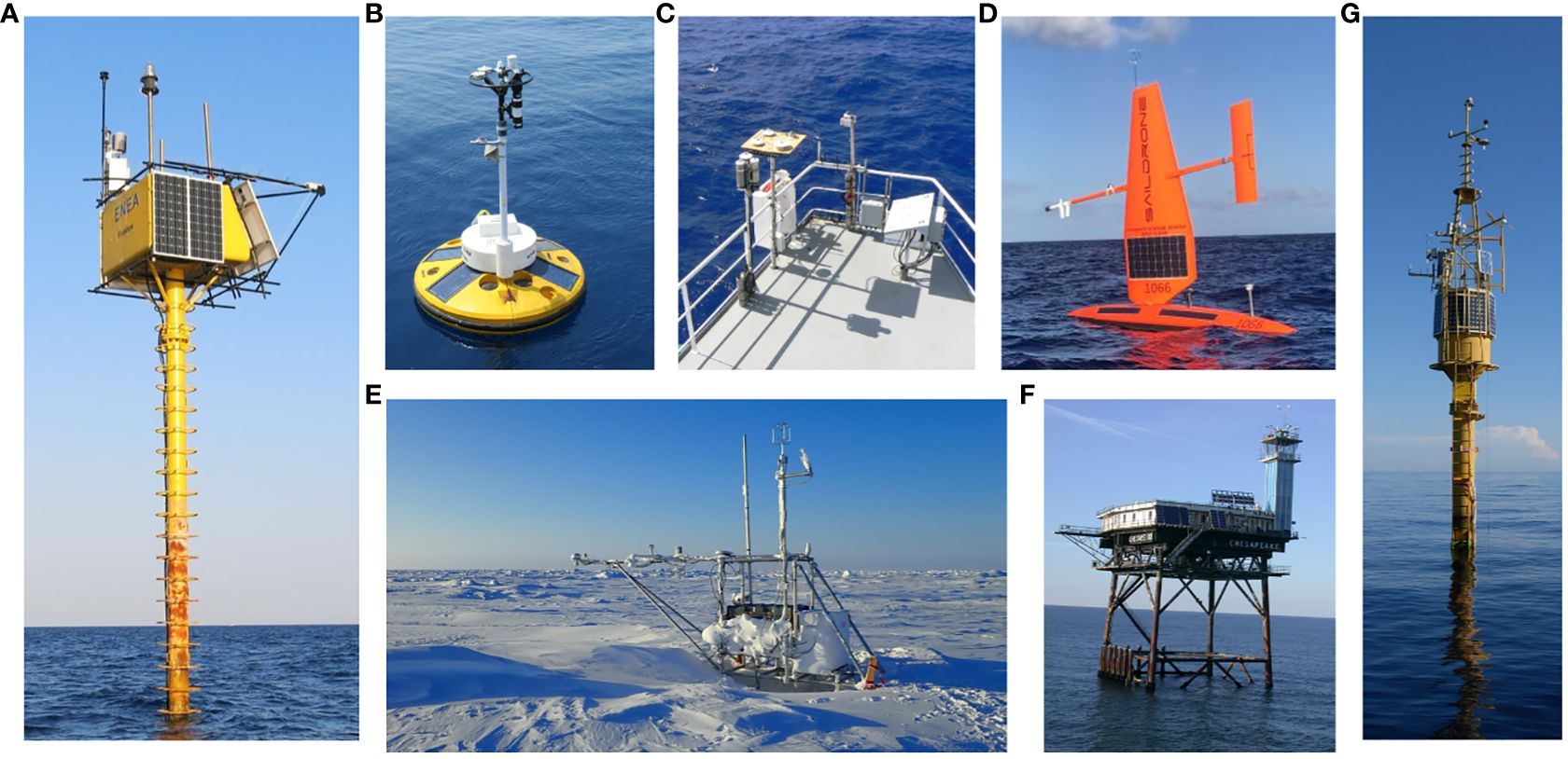
Figure 1 Examples of platforms used to measure the surface radiation budget. (A) Fixed tower at Lampedusa Observatory, Italy (photo by A. di Sarra); (B) Ocean Moored buoy Network for Northern Indian Ocean (OMNI) moored buoy in the Indian Ocean (photo by Dr. Martin V Mathew, NIOT, Chennai); (C) multiple radiometer systems on the deck of the NOAA ship Ronald H. Brown (photo by F. Bradley); (D) Saildrone USV as part of the Tropical Pacific Observing System (TPOS) (credit: Saildrone, Inc.); (E) sled on Arctic sea ice during the Multidisciplinary drifting Observatory for the Study of Arctic Climate (MOSAiC) field campaign (photo by C. Cox); (F) Chesapeake Lighthouse (BSRN site CLH); (G) Oceanografic Data Acquisition System (ODAS) Italia 1, a large spar buoy forming the W1M3A Research Facility that is part of the European Multidisciplinary Seafloor and water column Observatory- European Research Infrastructure Consortium (EMSO-ERIC) (photo by S. Pensieri).

Table 1

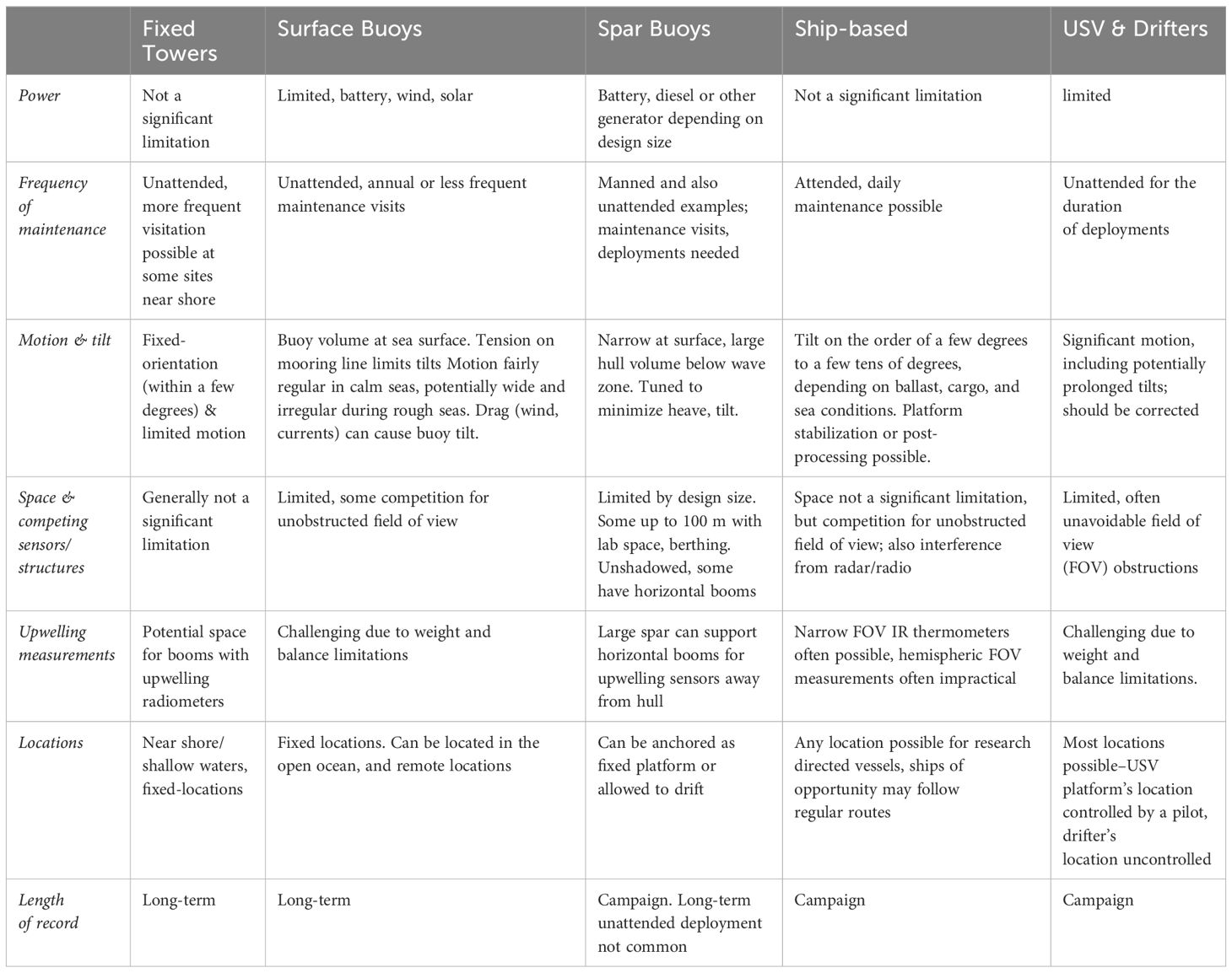
Table 1 Summary of observation platform limitations and opportunities.

We focus on measurements of downwelling SW, or solar, and LW, or infrared (IR) broadband radiation, and best practices for calculating or measuring the corresponding upwelling broadband components. We only briefly consider the ties between broadband and spectral measurements (e.g., Photosynthetically Active Radiation (PAR), ultraviolet (UV), or ocean color), though we hope that the broadband radiation best practices provided here will help spur additional discussion about synergies with spectral radiation measurement best practices. While we do not offer explicit recommendations for aircraft measurements in this paper, we discuss lessons learned from aircraft-based measurements for moving platforms and highlight the advantages of aircraft and Unmanned Aerial Vehicles (UAVs) to fill particular niches, such as upwelling observations.

A successful marine measurement strategy requires a variety of platforms capable of sampling different temporal and spatial scales in varied environmental conditions, that together can provide global coverage. The GCOS tiered network approach is a conceptual framing for how disparate platforms can be linked within the Global Ocean Observing System (GOOS) (e.g., Thorne et al., 2018). The network of OceanSITES (Send et al., 2010) fixed platforms provides long-term measurements at single locations within the open ocean. OceanSITES reference stations use the highest quality instrumentation and standards possible, giving the best potential counterparts to terrestrial BSRN stations, necessary for detecting changes in climate and validating remote sensing estimates of surface radiation. These open ocean reference stations along with coastal high-quality fixed tower stations, such as the Chesapeake Lighthouse Station (Figure 1F) that took measurements until 2016, can be capable of meeting at least GCOS ECV threshold uncertainty requirements of 10 W m^-2 as defined in ECV product requirement tables (GCOS, 2022, section 1.6). The ECV threshold uncertainty values are defined as the minimum requirement that must be met for the data to be useful for climate studies, with lower uncertainty values also defined for breakthrough and ideal requirements as well. Within the tiered network system of ocean observing platforms advocated here, long-term stations provide temporal variability measurements that can be linked to measurements of spatial variability from moving platforms like ships, USVs, and drifters. Ships provide unique advantages as a measurement platform because instrumentation can be maintained by staff who can monitor their performance, and generally have sufficient power and space to manage instrument level, and record measurements at high temporal resolution and in remote locations not often sampled by other systems. Ship-based measurements also face challenges related to shadowing by infrastructure, stack gas plumes and high energy radio frequency interference due to radar and radios. The advantages of being regularly maintained by personnel and fewer power and space limitations allows ships to be an important intercomparison standard when sailing on routes that pass moored buoys or moving autonomous platforms. Complementary to ships, new technologies like USV’s (e.g., Figure 1D) and drifters offer a lower-cost alternative to sample spatial variability where there are gaps in coverage, for short- (hours) or long-term (months to year) measurements depending on platform type. Other creative setups, such as the ice-bound buoys or sleds pictured in Figure 1E (Cox et al., 2023), can be tailored to meet the unique challenges of specific environments such as high-latitude regions (see also Lee et al., 2022). Surface-riding buoys as used by OceanSITES experience tilt; spar buoys are designed to minimize both heave and tilt. The community recommends establishing interoperability of surface radiation measurements from all ocean-based platforms, including USV and drifting buoys by quantifying uncertainties when following best practices relevant to each platform.

Additionally, the community recommends identifying the right permanent organizations or structures to maintain these best practices and coordinate the long-term development of the tiered network under development in OASIS.

A full characterization of the surface radiative budget requires accurate estimates of upwelling and downwelling SW and LW irradiances. Additionally, measurements of diffuse and direct components of downwelling SW irradiance allow for corrections for platform motion (Long et al., 2010), the calculation of fractional cloud cover (Long et al., 2006), and radiative effects (Long and Ackerman, 2000; Long and Turner, 2008). Downwelling irradiance can be measured directly from all ocean-based platforms discussed here. Conversely, upwelling flux measurements are rarely made on ocean platforms. For this reason, upwelling components are often calculated using ancillary measurements (Section 5). Downwelling radiation measurements including in the water as a function of depth were made from RP FLIP by (Simpson and Paulson 1977). Simpson and Paulson (1979) made simultaneous downwelling and upwelling radiation measurements from RP FLIP.

Current recommendations, challenges, and priority areas for improvement are addressed by measurement type for SW and LW radiation measurements (Sections 3-5), a brief nod to spectral measurements is made in Section 6, followed by recommendations for the handling and installation of sensors (Section 7), checking and improving data quality (Section 8), and calibration (Section 9). Within each section, identified needs for future research, community conversation, and experiments to determine best practices are italicized and underlined; these aspects are then summarized in Section 10. Current community recommendations are indicated in bold, with the list summarized in Section 11.

3 Downwelling shortwave radiation

SW radiation is defined as the full solar spectrum in the 0.1-5.0 μm wavelength range. In practice, most SW radiometers measure a range of approximately 0.29-3.0 μm, which contains 97% of the solar energy (WMO, 2018). The small amount of solar radiation not measured in the UV and near-IR is implicit in the calibration, yielding a negligible spectral inaccuracy. This section will describe instrument selection considerations related to accuracy and desired measurements, with additional recommendations for obtaining the best performance in the field in Sections 7-9.

3.1 Instrument selection

To achieve the BSRN target uncertainty requirements of 2% or 5 W m^-2 (Ohmura et al., 1998; McArthur, 2005), measurements of downwelling SW irradiance on land-based platforms incorporate redundant measurements. An unshaded and ventilated secondary-standard pyranometer is deployed to measure the downwelling SW radiation (we will refer to downwelling SW irradiance measurements from a single pyranometer as global SW radiation going forward). Redundant measurements are also made from summing the measured direct normal component with a pyrheliometer and the diffuse irradiance measured with a ventilated shaded pyranometer. We will refer to this way of measuring the downwelling total SW irradiance as the component sum SW going forward. This implementation requires a motorized sun tracker that keeps the pyrheliometer sensor normal to the incoming radiation and the diffuse pyranometer fully shaded.

Since the unshaded pyranometer is affected by the cosine response error, thermal offset and tilting, downwelling SW irradiance derived by the component sum method described above is generally considered more accurate than the global irradiance measured by a single unshaded pyranometer, although recent secondary-standard instruments have excellent performance with respect to the cosine response. On a moving platform, maintaining a sun tracker is generally not feasible, due to platform motion. Even fixed towers tilt a few degrees in response to wave motion (e.g., di Sarra et al., 2019). Upkeep of moving parts in the corrosive sea salt environment and power limitations further limit feasibility of maintaining a sun tracker on ocean platforms.

Pyranometers measuring global SW have improved significantly over time, and though they do not meet the accuracy of a tracker system, some models come close. Broadly, the specifications for a research-grade marine pyranometer should meet the highest standard for calibration uncertainty; have minimal directional dependency; and a fast response time.

The ISO 9060:2018 standards define a spectrally-flat Class A pyranometer that multiple manufacturers can currently meet, providing a starting point to evaluate the current state of the art for accuracy of SW irradiance sensors. We consider a number of the criteria in the current standard and how they are important for measurements from ocean-based platforms. For the purpose of measuring the radiation energy budget accurately, global SW measurements should be made with a thermopile-based sensor rather than one using a silicon (Si) photodiode sensor, or what is considered a spectrally-flat pyranometer in ISO 9060:2018 standards. Si-based sensors have a non-linear spectral response for SW wavelengths between 0.3 and 1.1 μm, and do not measure the portion of the SW spectrum between 1.1 and 4 μm (e.g., Vignola et al., 2016, 2017), which introduces a poorly-constrained bias dependent on sky conditions (e.g., atmospheric water vapor content). However, we note that Si-based sensors have a very high sampling rate which might be useful for experimental studies on the impact of tilts and motion on measurements.

Pyranometer measurements should prioritize minimization of cosine response errors, the directional dependence due to non-linearities in the thermopile response to the incident angle of incoming radiation, ideally through choice of sensors or possibly by corrections (described more in Section 8.3). This is particularly important for high-latitude measurements where the solar elevation angle is always relatively low. This is one of the largest error sources in previous generations of pyranometers (e.g., Michalsky et al., 1995), and an area where manufacturers have significantly improved technologies in recent years (e.g., Vuilleumier et al., 2014). Figure 2 shows the sensitivity of pyranometer calibration factors (responsivities) to solar zenith angle for different pyranometer models. As is typical for older models of pyranometers, the Eppley Precision Spectral Pyranometers (PSPs) vary by about 8% over the course of the day, while newer models from Kipp and Zonen (CM21, CM22) vary by 1-2%. Pyranometers are typically calibrated at a solar zenith angle of 45°, in clear-sky conditions, as shown by the blue vertical line in Figure 2. Thus, a pyranometer is generally most accurate at solar zenith angles of 45° and during overcast conditions when diffuse radiation is dominant, with positive and negative deviations from the cosine response partially balancing each other over the course of diurnal and seasonal cycles; the degree to which this cancellation occurs depends on deployment latitude.

Figure 2

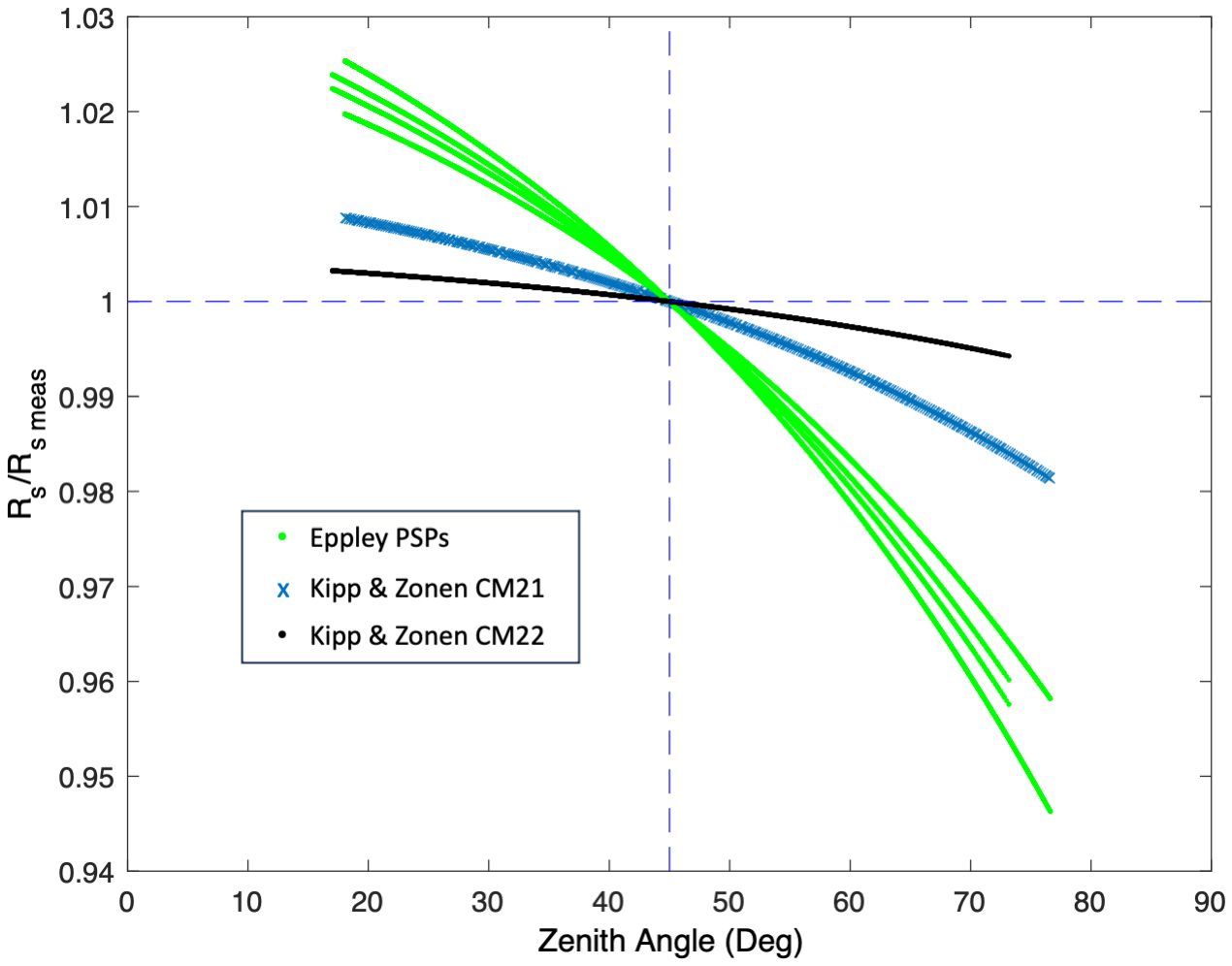
Figure 2 Ensemble of clear-sky calibration fits to different pyranometers from Boulder, CO and Woods Hole, MA rooftop deployments: four different Eppley PSP (green), Kipp and Zonen CM21 (blue), Kipp and Zonen CM22 (black). The measured irradiance equals the instrument voltage output divided by its responsivity, R_s, so here a value of R_s/R_{s meas} below 1 (above 1) indicates a lower (higher) instrument sensitivity at these zenith angles compared to a solar zenith angle of 45 deg.

Differences between downwelling SW measured by an unshaded pyranometer and the component sum can be easily found at land-based BSRN sites (Gueymard and Myers, 2009). A preliminary analysis comparing measurements from unshaded pyranometers and the component sum from BSRN data archived over the period 2000-2018, showed a median monthly RMSD of ~7 W m^-2 with first and third quartiles of ~4 and ~12 W m^-2, respectively, over all stations and months in the timeseries. The comparison was calculated for 1-minute measurements for each month and station in the archive. The average bias was nearly null, with first and third quartiles of -2 and +2 W m^-2, respectively. A range of instrumentation is used at BSRN stations, including pyranometers that meet ISO 9060:2018 Class A standards and older instrumentation with larger cosine errors.

Figure 3A shows NASA’s CERES SYN1deg data product (Rutan et al., 2015) calculated (hourly) SW irradiance down at the surface minus US DOE Atmospheric Radiation Measurement (ARM) station (SGP E13) observed values from component sum (black) and unshaded pyranometer (red) during clear skies. Results in 3a) show an overall positive bias (<1%) that linearly increases with respect to total SW as the cosine of the solar zenith angle [cos(SZA)] increases. However the calibration of the Eppley pyranometer to 45° solar zenith angle introduces non-linearity into the comparison resulting in larger negative biases for cos(SZA) > 0.8. Buoys historically, and in the foreseeable future, will likewise have unshaded pyranometers. Figure 3B shows calculated SW irradiance compared to buoy observations for the same clear sky conditions though collected from 46 different buoys. Overall bias is over 2% with significantly higher random error (RMS >10%), most likely associated with satellite cloud retrievals over tropical oceans using geostationary imagers and buoy motion. Again, the polynomial fit is significantly concave. These results are for hourly, ‘clear sky’ comparisons and suggest care should be used at high time resolutions as unshaded pyranometers give more meaningful values for daily averages and beyond. Likewise, the climate regime of a buoy may affect temporal averages if the buoy sits in a predominantly clear sky location. Indeed, many buoys in Figure 3B are located in tropical subsidence zones. Modern pyranometers have greatly reduced this solar zenith angle dependence though this is not the case for the historical record.

Figure 3

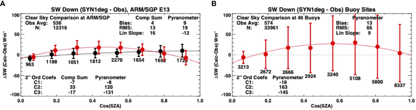
Figure 3 Differences between surface downward shortwave (SW) irradiance calculated hourly from the SYN1deg data product and observed hourly averages for comparison to global pyranometers (red) and component sum (black) at a range of solar zenith angles. (A) Results at the BSRN site at the ARM central facility “E13”. (B) Results from data drawn from 46 separate buoy locations for sufficient clear sky samples. Data are collected across 21 years (2000-2020) when the SYN1deg cloud fraction is< 1% for the 1° grid box where the site is located. Statistics are calculated in cos(SZA) bins, shown are the mean bias (circles) and +/- 1 standard deviation (vertical bars). 2^nd order polynomial fits are calculated for the entire data sets. All numbers are Wm^-2 except hour counts.

IR loss should also be considered as a potential systematic bias in measurements. While ventilated radiometers may have a reduced IR offset compared to non-ventilated ones, the thermal offset varies among different models of pyranometers and with environmental conditions and should be taken into account and properly corrected (Dutton et al., 2001; Gueymard and Myers, 2009; Wang et al., 2018). It is recommended that the thermal offset be mitigated if possible through use of radiometers with minimal offsets and ventilation when appropriate. However, since ventilation is difficult to maintain for pyranometers installed on many ocean platforms due to limited power availability, and funding for new instrumentation that mitigates thermal offsets may not be available, the thermal offset may represent a non-negligible bias in SW irradiance measurements. In these cases, correction of thermal offset in a SW radiometer should be applied, which requires simultaneous measurements of raw signals from a LW radiometer, reinforcing the need to include both sensors in the instrument suite. Methods for correcting for thermal offset are described in Section 8.2.

Response time is an important consideration on moving platforms, particularly when motion correction is applied to a measurement. Using an instrument with a faster response time than the 10-s minimum response time (time for 95% response) in the ISO 9060:2018 Class A standard is possible and desirable. Current thermopile-based pyranometers are available with a 3-s response time and could be created with less than 1-s response time (William Beuttell, personal communication). The response time of the pyranometer should be sufficiently fast to capture the sampling requirements of the scientific use of the measurements, which will be discussed more in Sections 3.2 and 7.4.

Finally, in the previous generation of instrumentation, sensor degradation was linked to degradation of the black coatings used on the thermopiles (Wilcox et al., 2001; Riihimaki and Vignola, 2008) causing potentially rapid drift from the initial calibration. It is recommended not to recoat sensors in response to sensitivity decline, as this decline happens most rapidly in the first year so recoating the sensors leads to a greater instability in the measurements. The sensitivity decline should be handled by further calibration when possible, otherwise it is recommended to retire the instrument from operations. Newer instrumentation with non-organic coatings do not experience the same rate of decline in sensitivity. Instrument manufacturers consulted here reported that sensor degradation is not likely to be significant after a potential sensitivity decline of ~0.5% in the first year of use. This stability is a specification listed in the ISO 9060:2018 standard which manufacturers need to meet. Current BSRN standards recommend regular calibrations (every 1-2 years). For older sensors this is necessary to maintain accurate calibrations. While newer sensors may not require such frequent calibrations for stability, regular checks also help identify any other instrument changes or repairs needed. Thus, currently regular calibrations (every 1-2 years) against a reference standard traceable to the World Radiometric Reference (WRR) are recommended following BSRN recommendations, as discussed in Section 9. We also recommend further conversations between the ocean community and BSRN to determine optimal calibration procedures for accuracy and practicality.

3.2 Correcting for tilt

When a pyranometer is not level it can change the apparent zenith angle of the direct solar radiation beam and thus alter the measurement significantly, particularly under clear skies and low sun angles when the aspect of the tilt is aligned with the direction of the sun. This introduces a challenge for measuring downwelling SW irradiance on moving platforms and care should be taken to mitigate the impact on measurements.

Platforms at sea can have both persistent tilts and varying tilts due to the impact of waves and swell on the platform. Changing cargo loads, fuel, and ballast tank levels, and trimming of the vessel can be the source of persistent tilts on ships that vary during a cruise. Surface buoys with wind loading and or drag forces on the hull and mooring line may have persistent tilts as well as pitch and roll. Systems on sea ice may be impacted by persistent, abrupt, and/or slowly-varying tilts from ice freeze/melt and dynamic activity.

We discuss here the three most common ways to deal with platform tilt and motion: averaging, stabilized platforms, and tilt correction post-processing. Which one is most appropriate for a given application depends both on deployment limitations and scientific priorities.

The wave motion that influences ocean platforms during calm sea conditions is fairly regular with a period on the order of 1-20 seconds (e.g., Toffoli and Bitner-Gregersen, 2017). If the desired scientific need of the measurement is for longer-term averages, such as daily or monthly average data from fixed towers or moored buoys for comparisons with model or satellite data, much of the variability caused by platform motion can be treated as a random fluctuation that will approximately cancel out with averaging (e.g., Colbo and Weller, 2009; di Sarra et al., 2019). A mean tilt to the sensor for certain wind and wave conditions, or due to the imbalance of the platform, however, will not average out and instead remains a systematic error or bias in the measurements. MacWhorter and Weller (1991) showed that a mean tilt of 10° can cause an error of 40% in the SW irradiance. If averaging is used as a means to mitigate platform motion, then a method is needed to also characterize any impact from mean sensor tilt relative to the direction of incoming solar radiation. The other two methods for tilt mitigation require additional instrumentation or equipment and may be cost-prohibitive or otherwise technically infeasible on some platforms. The unquantified systematic and random errors caused by waves and mean tilt may well make measurements unusable for some data users, such as the satellite community that needs measurements of known uncertainty for validation of derived products at the surface. Thus, the community recommends that best practices for characterizing mean tilt be developed through future intercomparison experiments.

Additionally, for averaging to be effective, the sampling must be of high enough resolution to subsample the period of motion and not selectively oversample one direction of motion over others. Both the instrument response time and the sampling frequency need to be considered when averaging. This is discussed further in Section 7.4.

Averaging may not provide sufficient accuracy for some scientific purposes or platforms, e.g. the need for higher temporal resolution data, such as 1-min average data needed for studying cloud effects, and platforms such as aircraft or USVs where substantial platform motion or mean tilts are too great for averaging to provide sufficient correction. Other mechanical or advanced post-processing methodologies are needed in these situations.

On platforms with sufficient power and weight capacity, such as a ship or larger aircraft, a mechanically stabilized platform can be used (Wendisch et al., 2001; Bucholtz et al., 2008). These platforms can keep an instrument level, compensating the ship motion, though active motion compensation may be more challenging in rough seas. Stabilized platforms can also be costly, and limited in the motion they can correct for so may not be practical in all deployments or wave conditions.

Another possibility is to use simultaneous measurements of sensor orientation and direct SW irradiance to calculate a correction to the downwelling SW. Because the orientation of the sensor primarily changes the measurement of the direct beam and not the diffuse irradiance, correcting downwelling SW irradiance requires knowledge of the separation of the irradiance components. A calculation described by Long et al. (2010) assumes that diffuse irradiance is isotropic and unchanged by tilt which they showed was a valid assumption when the instrument was within 10° tilt from horizontal. Equation 1, shows how to calculate total downwelling horizontal SW (G) from tilted measurements of downwelling SW irradiance (G_T), the cosine of solar zenith angle (${\mu }_o$), cosine of the tilt angle (${\mu }_T$), and the ratio of diffuse to direct normal irradiance (K).

$\begin{array}{ll}G = G_T \left(\frac{{\mu }_o + K}{{\mu }_T + K}\right)& (1)\end{array}$

The tilt angle is defined as the angle between a normal to the tilted surface and the incoming direct beam, as illustrated in Figure 4. Details of this derivation are found in Long et al. (2010). This correction has been successfully applied to the downwelling SW measurements from USV saildrones (Zhang et al., 2019), where the SW irradiance is measured at 5 Hz by an SPN1 Sunshine Pyranometer and the three-axis motion of the platform is measured at 20 Hz by a dual GPS-aided IMU VN-300.

Figure 4

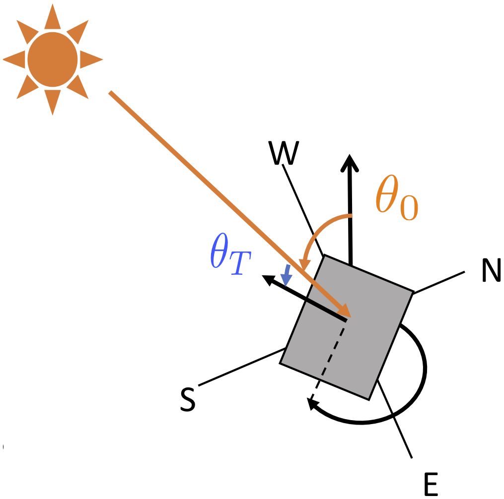
Figure 4 Diagram defining the tilt angle (${\theta }_T$) as the angle between the normal to the tilted surface and the direction of incoming radiation. The solar zenith angle (${\theta }_o$) is also indicated in the image.

3.3 Downwelling diffuse and direct SW components

In order to use the post-processing method of SW irradiance measurements, measurements of the partitioning between diffuse and direct SW radiation is necessary. Additionally, measurements of diffuse and total downwelling SW irradiance together can be used to estimate clear sky irradiances (Long and Ackerman, 2000), and cloud fraction (Long et al., 2006), and thus give more information for studies of cloud radiative effects and forcing. Also, the quantification of the diffuse and direct contributions helps separate the impact of clouds and aerosols on surface irradiance (e.g., Qiu, 2001; Riihimaki et al., 2009).

An example of an instrument capable of measuring the diffuse downwelling SW component on moving platforms including aircraft, ships, and an autonomous vehicle (Long et al., 2010; Zhang et al., 2019; Gentemann et al., 2020) is the SPN1 radiometer (Wood, 1999). The SPN1 instrument uses a fixed shading device that always shades at least one of seven sensors and keeps at least one sensor unshaded (see photograph inset in Figure 5), and thus has no moving parts. Another strength of the SPN1 instrument for moving platforms is that the small thermopile sensors have a fast response time of 200 ms (Delta-T Devices Ltd, 2019), which is sufficient to sample the impact of wave motion on the instrument’s effective zenith angle. The instrument design also minimizes IR loss, keeping offset errors to 3 Wm^-2 or less (Delta-T Devices Ltd, 2019).

Figure 5

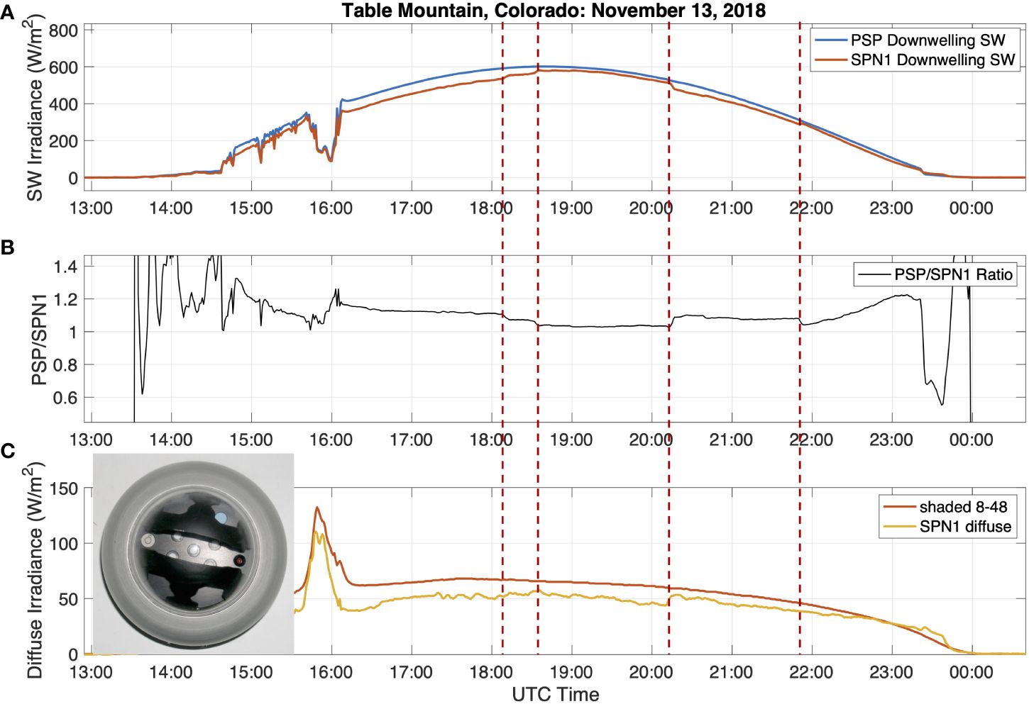
Figure 5 Downwelling SW irradiance measured by co-located PSP and SPN1 pyranometers for a sample day in Colorado (A), the ratio between those two measurements (B), and diffuse measured by a shaded Eppley 8-48 and an SPN1 (C). Vertical red dashed lines indicate step functions in the SPN1 measurements when the instrument switches between which of 7 sensors is used to measure the unshaded irradiance. Inset in the lower panel shows a photograph looking down onto an SPN1 radiometer showing the black shading mask and 5 out of the 7 thermopile sensors (small white circles).

However, due to the configuration and spectral range of the SPN1, step functions on the order of 10-20 W m^-2 can occur over the course of the day as different sensors become shaded and unshaded (Figure 5). Badosa et al. (2014), also found a 5-10% low bias in the diffuse SW radiation measurements depending on the conditions (e.g. Figure 5C). Thus, for the highest quality measurements, it is recommended that when a lower accuracy instrument is used to measure diffuse irradiance, a Class A pyranometer be fielded alongside as described in Long et al. (2010).

In addition to the SPN1, several deployments have used a fast-rotating shadowband on broadband and filter radiometers on ships, without the need for a stabilized platform (e.g., Reynolds et al., 2001; Witthuhn et al., 2017), though none were commercially available at the time of publication.

3.4 SW Instrumentation decision tree

To summarize the recommendations for the selection of SW instrumentation, we have created a decision tree (Figure 6). Class A pyranometers refer to spectrally-flat Class A pyranometers according to the ISO 9060:2018 standard. There are a number of pyranometers that meet this standard, with different specifications and sizes as well as power requirements. A list of some commonly used pyranometers in the BSRN network are listed in Table 2 to give readers an idea of the potential range of specifications for measurements meeting this standard, though this list should not be considered exhaustive.

Figure 6

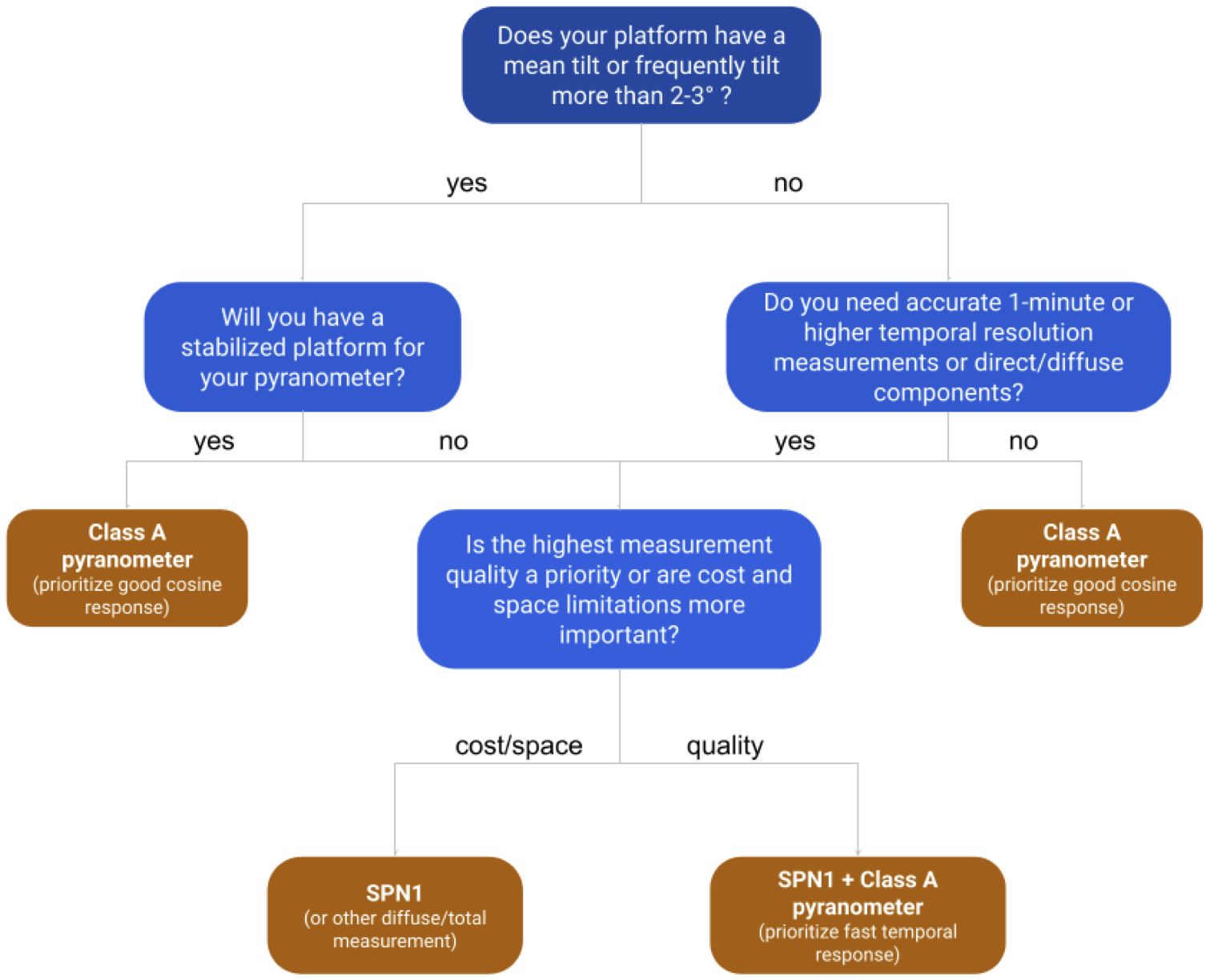
Figure 6 Decision tree showing recommendations (brown) for choosing instruments depending on platform and accuracy needs (blue). Examples of Class A pyranometers are given in Table 2.

Table 2

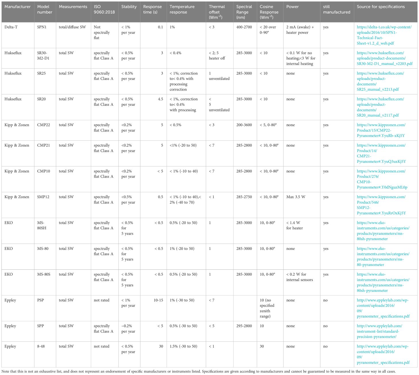
Table 2 Comparison of commonly used pyranometers.

4 Downwelling longwave radiation

Pyrgeometers measure the portion of the LW radiation spectrum from terrestrial infrared radiation. Pyrgeometer filters include wavelengths of approximately 3 to 50 μm. The small contribution of longer terrestrial wavelengths (~50-100 μm) is generally out of pyrgeometer filter ranges, but is approximately included in the measurements through the pyrgeometer calibration against the World Infrared Standard Group (WISG).

Detailed industry standards for pyranometers have largely been driven by the solar energy community, but there is no similar industry standard for pyrgeometers measuring LW radiation. There are consequently fewer instrument options available for LW measurements. The highest quality pyrgeometer sold by a manufacturer is generally the best option for climate quality measurements. Only a few LW instruments have been used in BSRN network measurements at the time of this publication, the most common of which are listed in Table 3. This list is not exhaustive but provides users an example of the specifications of high-quality pyrgeometers.

Table 3

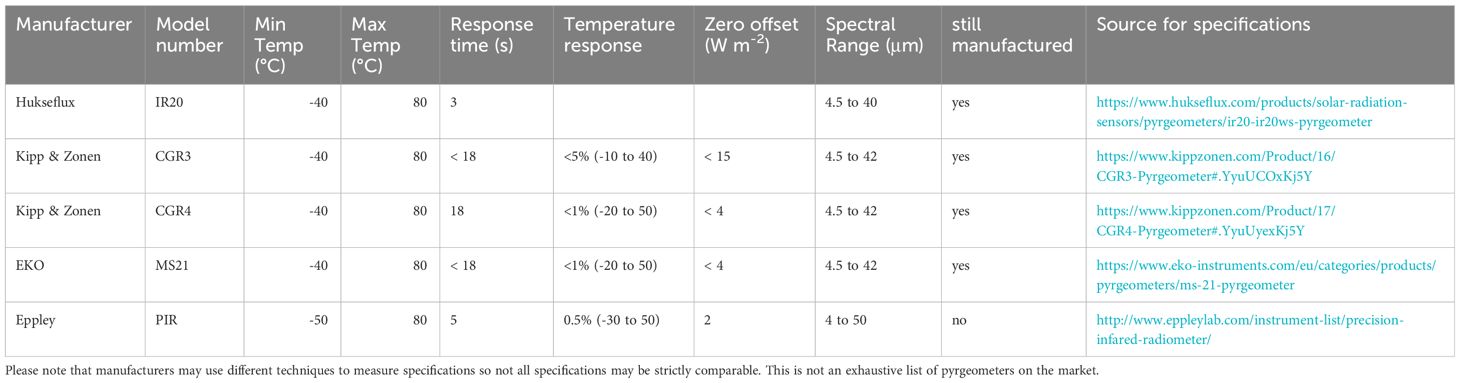
Table 3 List of pyrgeometers commonly used in BSRN, with specifications given by manufacturers listed for convenience.

Some of the challenges of pyranometer measurements, such as the dependence on the directional component of incident solar radiation, are not relevant to pyrgeometers. For small tilts (< 10°) downwelling LW measurements are not likely to be significantly affected by platform motion and the directional errors that plague pyranometers. Pyrgeometer calibration is an active field of research, which is discussed in Section 9.

Several BSRN recommendations are impractical for pyrgeometers on ocean-based platforms. Pyrgeometers on land are usually installed on a solar tracker with a shading device to block the direct solar component, which may heat the dome, cause heat exchange, and result in possible solar leakage (Meloni et al., 2012). Another land-based practice is to use ventilation to reduce heating of the instruments and reduce sedimentation of dirt or salt deposition due to increased airflow, which is only possible on platforms without significant power limitations. Meloni et al. (2012) found biases of up to 12 W m^-2 in unshaded Precision Infrared Radiometers (PIRs) compared to shaded pyrgeometers, and suggested possible corrections. Since these configurations are not practical on most autonomous ocean platforms, a key consideration in instrumentation choice is to use instruments with reduced dome heating effects. We recommend further work by the community to quantify the impacts of using unventilated and unshaded pyrgeometers of multiple manufacturers to aid understanding the uncertainty of the measurements, and whether standard corrections can be developed to improve measurement accuracy.

Response time in pyrgeometers varies among models from 3 to 18 s (95% response, Table 3). Because LW irradiance does not have a strong directional component like SW irradiance, its response time in most applications is less important and even 18 s adequately samples changing sky conditions for 1 min or longer averages, as clouds have a temporal decorrelation scale of ~15 minutes (Kassianov et al., 2005). However, in fast moving platforms like aircraft, faster sampling rates may be needed to capture spatial changes in sky conditions.

5 Upwelling measurements

Collecting hemispheric upwelling irradiance measurements is challenging over the ocean as most platforms, such as buoys and ships, do not have the potential to mount instruments far enough away from the platform to avoid significant interference from platform structures.

It is possible to make upwelling measurements on fixed platforms, though few exist. Upwelling measurements were taken for a number of years at the BSRN Chesapeake Light Tower, using a horizontally-oriented boom extending 9 m off the side of the platform (Figure 1F). Nevertheless, the measurements are not included in the BSRN archive due to (i) corruption of the upwelling SW flux by shadows cast by the tower; and (ii) errors in the LW measurement due to emission from the tower legs as they heated and cooled across the day. There are also plans to include upwelling measurements at the Lampedusa observatory in the future.

For future deployments on fixed platforms, the pyranometer should be mounted on the equator side of the tower (e.g. south side for towers located in the northern hemisphere) to minimize tower structure shadows. Painting the side of the tower mast facing south black may minimize the impact on the hemispheric radiation. The LW radiometer should be placed on the poleward side of the tower (e.g. the north side of the tower in the northern hemisphere), to reduce the impact of the daily heating/cooling cycle of the tower structure. The interference of the mast holding up the sensor arm increases with the mast diameter and decreases for increasing arm length such that the mast will take up a smaller portion of the field of view of the radiometer. The World Meteorological Organization (WMO) recommends (WMO, 2018) that upwelling radiometers should be placed at 1 or 2 m above a uniform surface and leveled. BSRN best practices over land use 3, 10, or 30-meter heights for upwelling measurements as higher measurements represent a larger area, improving measurement utility for the satellite community. On ocean platforms, these heights will most likely be set by infrastructure limitations. Aligning approximately with one of the BSRN heights would ensure continuity with land-based measurements and the farther distance from the ocean surface would reduce the impact of sea spray on the instruments, though choosing heights that reduce platform interference is likely a larger concern. Instrumentation recommendations are similar to those described in Sections 3 and 4 for downwelling irradiances.

In systems over sea ice, measuring upwelling irradiance, particularly SW, is necessary to quantify the surface radiation budget as albedos there are much higher and more variable than over the open ocean. This environment also has more potential for structures that can support upwelling measurements and some campaigns have featured ice stations to make such observations at staffed and semi-autonomous locations (e.g. SHEBA, Persson et al., 2002; CASES, Savelyev et al., 2006; N-ICE 2015, Walden et al., 2017). To increase station autonomy, sleds built for the Multidisciplinary drifting Observatory for the Study of Arctic Climate (MOSAiC; Shupe et al., 2022) successfully used booms for mounting upward- and downward-facing radiometers (Figure 1E; Cox et al., 2023), which was later repeated on a fully-autonomous spar buoy (Lee et al., 2022). Spectral albedo measurements have also been successfully measured from an autonomous platform (Nicolaus et al., 2010). These successes show the potential of autonomous sea ice platforms for measuring surface radiation.

Another promising platform for upwelling measurements in sea ice, ocean, and land environments are aircraft and UAV flights that can characterize the spatial variability of the surface and irradiance, giving better information about the surface energy budget and its impacts. Over oceans, UAVs have been shown to be an effective platform for measuring albedo and sea directional reflectance away from ships and other structures (Reineman et al., 2013; Zappa et al., 2020). Calmer et al. (2023) show that the aggregation scale of albedo over summertime sea ice from hemispheric broadband radiometric data occurs at ~50-60 m altitude, indicating that surface-based systems measuring sea ice are better at representing local temporal evolution and UAVs have a better potential to capture the horizontal mean albedo. Initial results show that sampling strategy is critical as spatial variability in upwelling SW and LW is significant (Zappa et al., 2020). To make the most accurate measurements there is a need for faster-response instrumentation and precise aircraft attitude. UAV stabilization can currently achieve less than 1° attitude change in a 10-s period when flying upwind, and roughly 1° for a 20-s period when flying downwind, though this is a function of air density. Improved UAV stabilization is recommended (and deliverable) to provide less reliance on tilt corrections described in Section 3.2. This is a growing area of research and is expected to provide fruitful new data for the community in the future.

When upwelling measurements are not available, they can be calculated from ancillary information as will be described in Sections 5.1 and 5.2.

The working group recommends intercomparison of reference datasets of upwelling broadband radiation measurements from crewed aircraft and UAVs to help the community better define the accuracy of current field deployments with calculated methods, including using different instrumentation for ancillary values, using estimations (e.g., from ships and land-based stations) described in Sections 5.1 and 5.2.

5.1 Upwelling SW calculations

For the purposes of calculating air-sea fluxes, Bradley and Fairall (2007), recommended calculating upwelling SW irradiance using a constant broadband albedo of 0.055. The date, time, and latitude-based albedo parameterization of Payne (1972) gives a better representation of albedo as a function of solar zenith angle and wind speed than a simple fixed value, and is now implemented in the forthcoming COARE version 4.0 bulk flux algorithm (James Edson, private communication).

Jin et al. (2004) developed a parameterized model for ocean surface albedo from observations taken during the CLAMS experiment (Smith et al., 2005) and a coupled ocean/atmospheric/sea ice radiative transfer model (Jin et al., 2006, 2023). The parameterization can be used to derive broadband ocean surface albedo as a function of the cosine of the solar zenith angle, wind speed, aerosol/cloud optical depth, and chlorophyll concentration. Hogikyan et al. (2020) compared albedo calculations from the CERES and ISCCP satellite products with a constant 0.055 albedo at equatorial, sub-tropical, and sub-polar buoy locations in the Pacific Ocean. The CERES dataset (based on the Jin et al., 2004 model) and the ISCCP model both include solar zenith angle, but use different inputs and models to describe sea surface conditions (e.g., foam, spray, glint, waves) as well as clouds and aerosol. Both models show reasonable agreement with a constant 0.055 albedo value in the tropics, but large spatial and temporal variability in surface albedo exists beyond simple zenith angle dependence (Hogikyan et al., 2020). A similar model to the Jin parameterization was recently developed by Wei et al. (2021). The model compared well with observations from the Chesapeake Light Tower and CERES ocean surface albedos and is optimized for the Rapid Radiation Transfer Model (RRTM) (Clough et al., 2005) which is the radiative transfer model used in a number of current GCMs. Nonetheless because of the complexity of the ocean surface there is a need for further work to test and improve albedo parameterizations for use in these calculations (Cronin et al., 2019).

5.2 Upwelling LW calculations

Rather than measuring upwelling LW, a more realistic approach for many platforms is to estimate upwelling LW from measurements of downwelling LW plus either the measurement of surface skin temperature or its estimate from a subsurface measurement used as input in an algorithm that accounts for cool skin and warm layer effects (Fairall et al., 1996, 2003). Bradley and Fairall (2007) recommend using an emissivity ($\epsilon$) of 0.97 and calculating upwelling LW using Equation 2:

$\begin{array}{ll}L{W}_{up} = \epsilon \sigma T_s^4+ (1-\epsilon )L{W}_{dn},& (2)\end{array}$

where $\sigma$ is the Stefan-Boltzmann constant, $T_s$ is the ocean surface skin temperature (in K), and $L{W}_{up}$ and $L{W}_{dn}$ are upwelling and downwelling LW irradiance, respectively.

This calculation requires accurate skin temperature estimation or measurements (Donlon et al., 2014). Ideally, the skin temperature is measured directly with downward looking radiometers, or IR thermometers that are corrected for reflected radiation by a separate upward looking device or the same device that is occasionally rotated to look upwards (Donlon et al., 2014). More typically, a thermistor is used to measure the temperature at some depth. Thermistors that can be towed very close to the sea surface (e.g., a sea-snake) require an adjustment for cool skin (on the order of 0.25°C). Thermistors at depth (e.g., from surface moorings or drifters) require correction for diurnal warming and then adjustment for cool skin (Fairall et al., 1996; Marullo et al., 2016). A vertical array of temperature sensors may constrain estimates of the warm layer but not the cool skin since it is very shallow (<= 1 mm).

6 Spectral measurements

Solar radiation penetrating the air-sea interface is absorbed at wavelength-dependent depths: long wavelengths are absorbed more quickly than short wavelengths primarily due to absorption by pure seawater. It follows that longer wavelengths (reds) are absorbed in the upper part, and at 40 meters depth, seawater has absorbed virtually all the red visible light; shorter wavelengths (blue light) are able to penetrate beyond 40 meters in clear, typically oceanic, waters. The depths of heat absorption are critical for determining the stratification and the temperature of the ocean surface layer. The absorption profile depends upon optical properties of the water (Ohlmann et al., 2000; Light in the Ocean). However, best practices for measurement of penetrative radiation by optical sensors in the water is beyond the scope of this paper. For more discussion on ocean measurements of penetrative solar radiation see references (e.g. Lotliker et al., 2016; Amber and O’Donovan, 2018).

Energy from sunlight is also critical for supporting marine life through photosynthesis, and has a spectral component. Solar radiation in the visible wavelength band of 400 to 700 nm is considered Photosynthetically Active Radiation (PAR) and is the most important source of energy for plants. PAR sensors are generally less expensive than broadband solar radiation sensors and provide the spectral information needed for biological applications at the target wavelengths. PAR quantum sensors are responsive to all photons in the 400-700 nm spectral range, cutting radiation below 400 nm and above 700 nm. This definition has been adopted after McCree (1972). Although the ideal spectral response is flat, commercial quantum sensors have spectral responses slightly deviating from the ideal and with cutoff wavelengths different from 400 and 700 nm. In addition, they are affected by a cosine response, that is an angular response deviating with the cosine of the incoming direction of radiation. These are the main source of deviations from one sensor to another measuring PAR (Ross and Sulev, 2000). Most atmospheric PAR sensors have a silicon photodiode detector, are lightweight and have a wide operational temperature range, making them suitable for installation in different environments and platforms. Underwater PAR measurements can be performed with either lightweight, small sensors, highly resistant to corrosion, or by more sophisticated instruments equipped with mechanical anti-fouling systems for long-term monitoring on moorings and buoys.

In addition to PAR, ocean color measurements for biogeochemical work need to observe additional wavelengths from the ultraviolet (UV) to the short-wave infrared (SWIR), with high spectral resolution. This spectral resolution is needed to better separate the signal from within the ocean (the desired signal) from that reflected from the surface and the atmosphere in remote sensing measurements, which is particularly challenging over turbid waters for coastal and inland water applications (GOOS Panel, Essential Ocean Variable (EOV): Ocean Colour, 2018). The distribution of UV and visible solar radiation regulates ocean biogeochemical cycles of carbon, nutrients, and oxygen (Frouin et al., 2018); among a wide range of applications, ocean color measurements offer a quantification of the global distribution of ocean phytoplankton (indexed by the chlorophyll-a concentration and responsible for roughly half Earth photosynthesis, Field et al., 1998) as well as specific blooms including those from harmful algae (Blondeau-Patissier et al., 2014) or coccolithophores (IOCCG, 2014). The sensors required for spectral measurements in the field differ from those used for heat budget analyses, and therefore require separate best practices (e.g.,Mueller et al., 2003; Frouin et al., 2018; IOCCG, 2019; Ruddick et al., 2019a, b), which have been and are continuing to be developed under the International Ocean Colour Coordinating Group (IOCCG).

While identifying best practices for these spectral instruments is beyond the scope of this paper, connections between the physical and biological communities would be of great value as interdisciplinary process studies and interdisciplinary measurement platforms continue to grow through activities such as OASIS and OneArgo (Owens et al., 2022), and should continue to be considered in future best practice efforts. One particular connection worth noting here is that the quantities derived from ocean color measurements that are widely used by the biological community also impact the ocean surface albedo which is fundamentally important for radiative energy budgets (Enomoto, 2007; Wei et al., 2021). An innovative approach being used by the ocean color community is separating the upwelling irradiance reflected at the ocean surface and the portion of upwelling irradiance that is scattered within the water. That is, quantifying the water leaving albedo, defined as the ratio of upwelling irradiance coming from scattering within the water to the downwelling irradiance. Numerical simulations based on inherent optical properties that calculate water leaving albedo outperform those based only on chlorophyll-a concentration, therefore they can improve model calculations of ocean albedo, as shown using satellite estimates of water leaving albedo from the Visible Infrared Imaging Radiometer Suite (VIIRS) (Yu et al., 2022). Considering their hyperspectral nature, the ocean color measurements given by the upcoming PACE (Plankton, Aerosol, Cloud, ocean Ecosystem, Werdell et al., 2019) mission might also provide interesting connections with the physical community.

7 Handling of sensors and installation setup

In the 2020 OBPS workshop, the surface radiation working group identified capacity building as a high priority (Cronin et al., 2021). Field expertise is too often developed by trial and error and specific details about sensor handling, installation or calibration remains ‘in-house’ knowledge. The community requires a method to provide current information and the ability to distribute recommendations and best practices to new users; this in turn will promote community-wide early adoption and standardization of practices and ultimately result in high-quality radiation measurements. This paper hopes to clarify best practices and recommendations as a step towards that capacity building. This section contains recommendations for sensor installation, maintenance, and data collection. This effort builds on earlier work, such as that from Bradley and Fairall (2007), but incorporates recommendations from new platforms, instrumentation, and practices that have developed in recent years.

7.1 Installation of instrumentation

The location of instrument installation is critical and should be chosen to reduce or eliminate shading and thermal emission of platform structures and minimize radio frequency interference from antennas and other electronics. Sensors should be positioned on the highest point possible to avoid shadows and IR heating. On ships, it is also recommended that radiometers be placed forward of the stack, as stack gas can be sufficiently warm to produce IR radiation in a measurable range. However, the highest level on a platform is also often desirable for other meteorological instruments that are particularly susceptible to flow distortion, such as anemometers and rain gauges. If space constraints make it impossible to avoid having objects in the field of view of the radiometer, it is recommended to take into account the cosine response of the sensor (i.e., have the object as low in the radiometer’s field of view as possible) and consider the reflectivity/emissivity of the object. For instance, one can calculate the impact of structures on LW measurements using the formula in (Bradley and Fairall 2007, Appendix C). They show diagrams of potential radiometer placement on board ships that include considerations that minimize shading/heating, but also keep instrumentation accessible to technicians who clean and maintain them. If it is not possible to eliminate the influence of platform structures, another way to mitigate this problem is by installing a second radiometer that will be shaded by platform structures at different times and combining the two datasets. If shading cannot be avoided, compromised SW data should be removed from the dataset when possible.

Additionally, as sensor leveling is critical, care should be taken to align the sensor with the waterline to remove mean tilt biases. When calculating a tilt correction, as described in Section 3.2, the sensors should be aligned with respect to what the tilt sensors call level.

When considering locations for radiometer, particularly on ships or large fixed ocean platforms, it is possible to conduct Electromagnetic Interference (EMI) testing to determine the “cloud” of EMI influence by other systems on the platform. Such testing can determine the level of EMI between nearby satellite, radio, or other EM emitting systems at the site proposed for the radiometers. If EMI is moderate to severe, enough to break up or mask the radiometer signal, then an alternate location for the radiometers should be chosen.

7.2 Ventilation

The BSRN standards dictate using a fan to ventilate pyranometers and pyrgeometers to minimize IR loss biases and reduce dust, frost, and condensation on domes. Using ventilators is impractical on many ocean platforms due to power and space limitations. However, the use of ventilators on platforms where space and power are not limiting factors, such as ships, should be further explored, especially ships that frequent high-latitude locations where heating and ventilation may prove necessary in freezing conditions. If ventilators are not used, some field experience suggested that removing the sun shields may be advisable to reduce uneven heating of radiometer bodies at low sun angles. Tests are recommended to determine the relative impact of these three configurations: ventilated, unventilated with a sun shield, and unventilated without a shield to make further recommendations about when these configurations are advisable.

In high-latitude locations, such as over sea ice, where freezing conditions are common, ice-mitigation is needed to avoid instantaneous errors of +/- 100-200 W m^-2 (SW) and +60 W m^-2 (LW) (Cox et al., 2021). Mitigation is typically achieved with a combination of heating and ventilation, but if carefully-designed, ventilation alone is sufficient, which reduces power consumption (Cox et al., 2021).

7.3 Modifications

Some groups use off-the-shelf (i.e., commercial) instrumentation and data loggers to acquire output directly from instrumentation, while others use modified electronics and instruments for better performance in ocean environments. This is particularly true for power-limited, unattended platforms like buoys and USV.

Thermopile output voltages from both SW and LW radiometers are on the order of 10 µV per W/m² of incoming radiation or less, thus these small voltage signals need to be amplified prior to digitization. Due to the smaller signal out of a thermopile for LW measurements, there is a greater need to quantify and control the stability and accuracy of amplifiers and other signal conditioning electronics than with pyranometers. Radio frequency interference can also introduce noise to the signal. When building electronics to amplify and digitize thermopile output for datalogging, it is recommended to keep the amplifier and digitization near the transducer. Inline amplifiers in the signal cable should be avoided.

Some analog LW radiometers used internal circuitry to combine case and dome thermistor readings with thermopile output to provide a voltage as a measure of the downwelling LW. Users found that recording the thermistor readings and the thermopile output for use in computing downwelling LW yielded more accurate results.

Marine use exposes radiometers to salt spray and visits from sea birds which leave guano behind. Some users replace the stock housings (holding the thermopile and dome) with more corrosion resistant material (for example, replacing aluminum with stainless steel) and/or apply coatings to exposed metal surfaces. As these changes may influence the solar heating and heat held by the housings, it is important to quantify any change in radiometer performance by comparison with unmodified standards. To reduce birds roosting on radiometers, vertical rods have been added to a ring fitted around the radiometer case (Figures 7B, C); if this is done the impact of shadowing and of infrared emission in the near field of the radiometer should be assessed.

Modifications for ventilation to reduce thermal gradients across the radiometer and for mitigation of dew/frost on the dome have been made and should be assessed for impact on performance and calibration.

Additionally, vendors are now marketing digital pyranometers and pyrgeometers and we think it would be valuable to test these for ocean use. A major recommendation of the surface radiation community working group at the 2020 OBPS workshop was to work with manufacturers to standardize instrument modifications for widespread marine application (Cronin et al., 2021).

More discussion in the community about best practices for instrument modification related to developing electronics for low-power environments and adequately sealing instrumentation and electronics for robustness in ocean environments is recommended, including the ability to pass along these needs to instrument manufacturers, who may be able to provide custom-built instrumentation for marine environments, making more accurate measurements more accessible and reproducible.

7.4 Sampling rates

BSRN standards for land-based irradiance measurements require 1-minute averages (minimum, maximum and standard-deviation) of 1-second samples, and recommend that operators record the raw 1-second data for reprocessing purposes, if possible. Sampling rates on ocean-based platforms are not standardized, and it is recommended that sampling-rate standards be developed for better consistency across platforms.

Two fundamental scientific frequencies need to be taken into account in order to determine appropriate sampling rates: the typical period of wave motion (on the order of a few seconds), and the typical timescales of growth and dissipation of convective clouds (on the order of minutes).

If a tilt correction is going to be applied, the sampling rate needs to be at least twice the frequency of platform motion, and coincident with measurements of pitch, roll, and heading. As periodic wave motion in calm seas typically has a period of 1-20 s (e.g., Toffoli and Bitner-Gregersen, 2017), the sampling rate will generally need to be greater than 1 Hz for tilt correction. As discussed in Section 3, it is important to use a SW sensor with sufficiently fast time response to capture this motion. The corrected high-temporal resolution data can then be averaged to a more practical resolution like 1-minute data for most purposes, which also should capture changes in radiation due to cloud evolution overhead.

If the primary scientific scope of the measurements is long-term averages, the sampling rate needs to be sufficiently high to not alias the measurement by selectively sampling a given orientation relative to the wave slopes. In this case, an instrument with a longer temporal response may naturally perform some of that averaging if its temporal response is slower than the platform’s motion that houses the instrument. Sensitivity tests of the sampling rate with instruments of different temporal response could be done to help determine requirements for sampling rate.

7.5 Maintenance for marine environments

Three recommendations for maintenance in marine environments were deemed particularly important by the working group. First, instruments need to be packed with care so that the domes are not broken during transport as damage to domes will compromise the measurements (e.g. Figure 7A shows the results of improper packing).

Figure 7

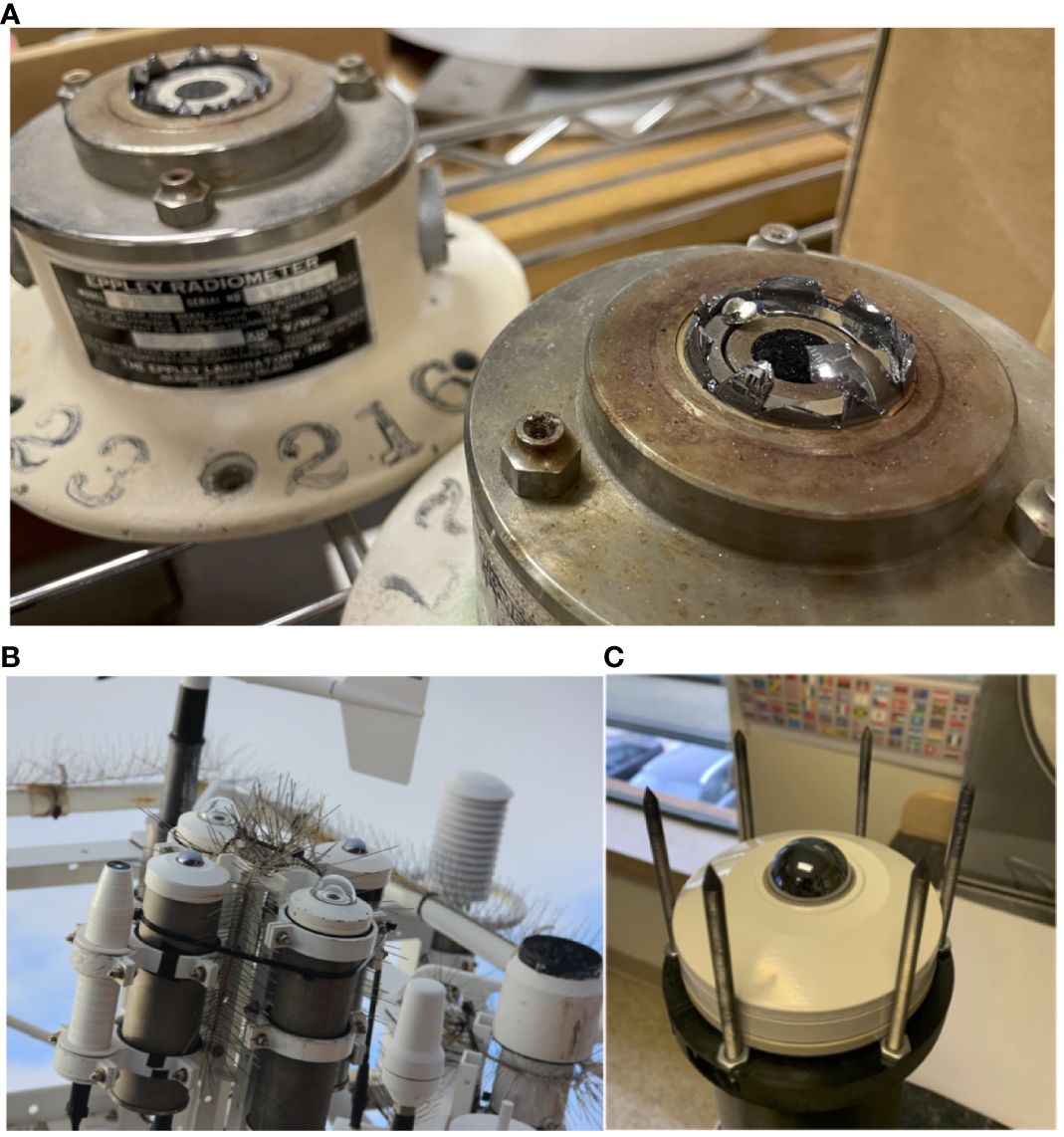
Figure 7 (A) Photograph of Eppley PIR pyrgeometers with broken domes from improper packing when shipping. Photo credit L. Riihimaki. Lower photos show two examples of bird deterrent spikes used on unattended systems. The older design (B) was found to be insufficient to keep birds from sitting on and soiling sensors, so a new methodology (C) is being tested to see if it is effective and does not overly interfere with measurements. Photo credit R. Weller.

Second, to take good measurements, moisture within pyranometers and pyrgeometers needs to be kept to minimal limits. In attended instrumentation, such as on ships, this can be accomplished by changing desiccant regularly. On unattended platforms, instruments must be robust enough to seal out all moisture for extended deployments. This may require instrument modifications if the desired instrument does not meet this criterion.

Finally, cleaning of sensors from dust, aerosols, salt deposits, bird droppings, and biofouling is important to maintain good measurements. On ships and other attended platforms, daily cleaning is recommended, with weekly cleaning at a minimum. Cleaning can be done with a soft cloth or delicate wipes, using distilled water in warm temperatures, or with alcohol when temperatures are cold or for soiling due to organic or oil-based substances. More details are included in the Supplementary Materials, under ship-based recommendations.

On unattended platforms, such as buoys, cleaning may only be able to be performed during deployment of instruments, or otherwise naturally when rain occurs. Since rain occurs at different intensities and frequencies across the globe and throughout time (annually, seasonally, subseasonally, diurnally), cleaning by rain cannot be counted on all the time or at all locations. Redundant measurements can help assess some quality control issues such as biofouling or a bird sitting on an instrument that typically do not impact both instruments simultaneously. Additionally, some automated cleaning systems are being designed for fixed-platforms, and it is recommended to test these systems for their ability to keep domes clean and give more insight into the magnitude of this cleaning error on systems that can’t be cleaned.

Power limitations may make it impractical to deploy automated cleaning systems on many unattended platforms. In these cases, it is important to be able to quantify the possible error associated with dome soiling. One practice that can help quantify this error is to calibrate instruments before and after cleaning at the end of a deployment (Colbo and Weller, 2009). This may not be possible for drifters which are typically not recovered post-deployment. Waliser et al. (1999) investigated the effect of dome cleaning on SW irradiance measurements in the North Atlantic Ocean. They recalibrated the SW radiometers after substitution on the buoys following 8-month unattended deployments before and after cleaning, and found differences smaller than 2%. This can be done with side-by-side tests using instrumentation on a ship when buoys are being serviced, or done at a calibration facility after radiometers have been recovered from the field.

These tests alone are not likely to fully quantify the errors as sensors are subject to changing conditions such as rain and contaminants don’t necessarily build up at a measurable or predictable rate over time. Observation sites which are not far from stations where reference measurements are carried out on land, such as for the Lampedusa observatory (e.g., di Sarra et al., 2019), give the opportunity to investigate systematic differences. Di Sarra et al. (2019) compared SW irradiance measurements made at the Lampedusa observatory with those made on the island of Lampedusa, at 15 km distance, where regularly cleaned instruments are operational. They found that the average effect of dome cleaning on ocean observations at Lampedusa is negligible. Some land-based tests also showed fairly negligible (less than 1%) changes in SW irradiance measurements from pyranometers when assessing 2 years of data from 25 sites that were cleaned every 2 weeks (Myers et al., 2001). Geuder and Quaschning (2006) tested the impact of pyranometer soiling in dry conditions with more mineral dust deposition and infrequent rain for periods of time up to over 100 days and found an average of about 1% error due to lack of cleaning, though with individual cases with errors of up to 5% from heavier soiling, and one case with a 17% error due to bird droppings on the pyranometer dome. Foltz et al. (2013a) studied the impact of dust deposition on measurements made on a moored buoy west of tropical Africa, where intense desert dust transport and deposition occurs. They found a negative bias in SW irradiance with respect to satellite analyses and model calculations, and estimated a 14% decrease in SW irradiance produced by dust deposition by comparing a freshly calibrated sensor with a dirty one removed from the buoy. Foltz et al. (2013a) also used precipitation measurements on buoys as an indicator of when domes would have been cleaned by rain. This might be a potential way to evaluate measurement uncertainties in locations with high soiling.

7.6 Instrument changes on unattended platforms

For the case of instrumentation that is unattended in the field for long periods of time, such as on buoys, care should be taken to check the impact of environmental degradation on the measurements. This information can help better quantify achievable measurement uncertainty in the field.

When possible, comparisons against freshly calibrated instruments on the same or nearby platforms should be performed before unattended instruments are retrieved for maintenance and calibration. This gives a field comparison against a well-maintained instrument. This can be done with overlapping deployments on ships or new surface moorings alongside those that have been in the water for an extended period.

Additionally, calibrating instruments retrieved from the field before any cleaning or maintenance is done can give an estimate of the impact of soiling. The condition of the instruments should be documented and preserved, including material deposited on the dome.

8 Best practices for data quality and processing

8.1 Monitoring data quality in the field

Broad checks can be made with data in the field to ensure values are reasonable. Measurements should be taken 24 hours a day when feasible and nighttime offsets examined to look for reasonable values. Because of the thermal offset experienced by some pyranometers, values will often be negative at night, particularly under clear skies when the temperature difference between a clear sky and the thermopile is greatest. The magnitude of these negative offsets depends on the atmospheric conditions and the instrument in use, but generally is no more than a few W m^-2 in newer pyranometers that meet ISO 9060:2018, Class A standards. For older generation instruments like the Eppley PSP, these offsets may be larger (up to 10 Wm^-2 or even larger).

Measurement values should be checked using expected ranges of values for each variable. While these limits can be set more specifically for a given location and climatology in post-processing, as described in Section 8.4, in general the downwelling SW irradiance values should be 0 at nighttime, average to no more than 1200 W m^-2 at solar noon. On clear days, SW irradiance measurements should exhibit a smooth diurnal curve. On cloudy days, SW values should generally decrease compared to clear skies, though cloud effects on partially cloudy days may cause downwelling SW measurements to exceed 1500 W m^-2 for short durations up to 10-20 minutes.

Downwelling LW irradiance values can range from 40 to 700 W m^-2 (Long and Shi, 2008), although smaller realistic ranges can be defined at specific latitudes, with higher values in warmer, humid locations like the tropics and lower values in dryer, colder locations like polar regions. Downwelling LW values should increase when the sky is cloudy (particularly in the presence of low, optically-thick clouds).

It is technically possible to install LW and SW radiometers for which the sign of the recorded voltage is opposite the intended measurement but the instrument is working properly. It is good practice to reconcile the expected actual signs of the voltages with expected radiation values at radiometer installation. As discussed in Sections 7 and 8.4, it is advantageous to deploy duplicate SW and LW sensors on the same platform or in overlapping deployments of new and existing to-be-recovered moorings so that outputs can be checked and corrected if needed.

Finally, it is recommended that the community create climatologies or climatology tools to show typical values by location, time, and relationships between variables to make it easier to quality control data consistently.

8.2 IR loss correction in pyranometer measurements

Negative offsets in pyranometer measurements caused by IR loss by the thermal exchange between an all-black detector and the atmosphere can be reduced through instrument engineering or removed through post-processing adjustments to the data. IR loss is the cause of negative pyranometer output at night, though it can also lead to a negative bias during the day. When simultaneous measurements from a pyrgeometer are available, this bias can be corrected. Several calculations are available for this correction. In the previous version of the BSRN manual (McArthur, 2005), no consensus was reached about which correction method should be used, though it was recommended that regardless of the methodology used, adjusted measurements should be thoroughly checked at each installation. We recommend working with the BSRN community to determine when and what IR loss corrections should be applied for the next manual.

One widely used estimate of thermal offset uses measured pyrgeometer detector flux, case, and dome temperatures (Dutton et al., 2001). This correction determines regression coefficients ($b_0, b_1, b_2$) empirically by fitting pyranometer and pyrgeometer measurements at night, when solar zenith angles are larger than 108° (Equation 3).

$\begin{array}{ll}os = b_0+b_{1}NetIR+b_2\sigma (T_{dome}^4-T_{case}^4)& (3)\end{array}$

Where $os$ is the offset in W m^-2, $NetIR$ is the flux measured by the pyrgeometer detector (the irradiance signal that comes from the pyrgeometer alone without correction terms from case or dome thermistors), $\sigma$ is the Stefan-Boltzmann constant, and $T_{dome}^{}$ and $T_{case}^{}$ are the dome and case temperatures of the pyrgeometer in K. For some models of pyrgeometer only the case temperature is measured and the dome temperature is assumed to equal the case temperature so the last term in the equation is effectively zero.

Other simpler forms of the offset corrections correlate the pyranometer offset with the pyrgeometer detector flux only (e.g., the detector only correction in Younkin and Long, 2003), or with the pyrgeometer IR signal (e.g., Wardle et al., 1996).

Much of the research on IR loss correction was done using the previous generation of pyranometers. A recent study by Wang et al. (2018) examined the impact of applying a thermal loss correction on newer and older generation pyranometers, ventilated and unventilated. For newer pyranometers, the average thermal offset was quite small, generally<2 W m^-2. The study examined the magnitude of the deviation of global pyranometer measurements from downwelling SW irradiance measured by the component sum method. Instrument-specific recommendations were then given for the best thermal offset correction method, including that described in Dutton et al. (2001), a detector-flux only correction, or no correction.

8.3 Fix cosine response through post-processing

The cosine response of a SW pyranometer can be significantly non-linear and yield significant errors when using a single calibration value, due to the dependence of the measurement on the direction of illumination. This is particularly true of older generation pyranometers. Newer pyranometers have more fully minimized and quantified this error so that, for example, pyranometers meeting Class A specifications given in ISO 9060:2018 should have cosine response errors<10 W m^-2 (as discussed in Section 3.1).

One possible approach to mitigate this error in downwelling SW measurements is to calibrate pyranometers with respect to solar zenith angle. However, the instrument cosine response is dependent on sky conditions so it isn’t straightforward to determine how to apply that calibration. When a single calibration coefficient is used, set at 45° incidence, the pyranometer will overestimate solar irradiance during clear sky conditions when the solar elevation is low (i.e., near sunrise and sunset) and underestimate irradiance when the solar elevation is high. This can be corrected to some extent if it is characterized as illustrated in Figure 2. However, this correction is only strictly valid for clear sky conditions when the majority of the signal comes from the direct normal irradiance. Diffuse radiation generally does not have a directional component, and a calibration at 45° is more accurate for these times (see argument in Vignola et al., (2017), Chapter 6). Therefore, for an accurate correction, it must be determined whether there is a direct component to the measurement. Most land-based measurements do not use a zenith angle dependent correction because pyranometer-measured downwelling irradiance is considered a secondary measurement and more accurate measurements can be made with the sum of the direct and diffuse measurements.

More work should be done to test the impact of a solar zenith angle dependent calibration for ocean platforms, to fully understand under which conditions it would be recommended.

8.4 Quality assessment and quality control

8.4.1 Redundant measurements

One of the most effective ways to perform data quality control (QC) and prevent data loss is by taking redundant measurements (e.g., Colbo and Weller, 2009). Figure 8 shows an example of how shading can be identified by systems on the port and starboard sides of the supply vessel Aurora Australis in the Measurements of Aerosols, Radiation, and Clouds over the Southern Ocean (MARCUS) field campaign (McFarquhar et al., 2021). In the afternoon, the measurements on the port side show a smoother curve, but those on the starboard side show intermittent dips from shading.

Figure 8

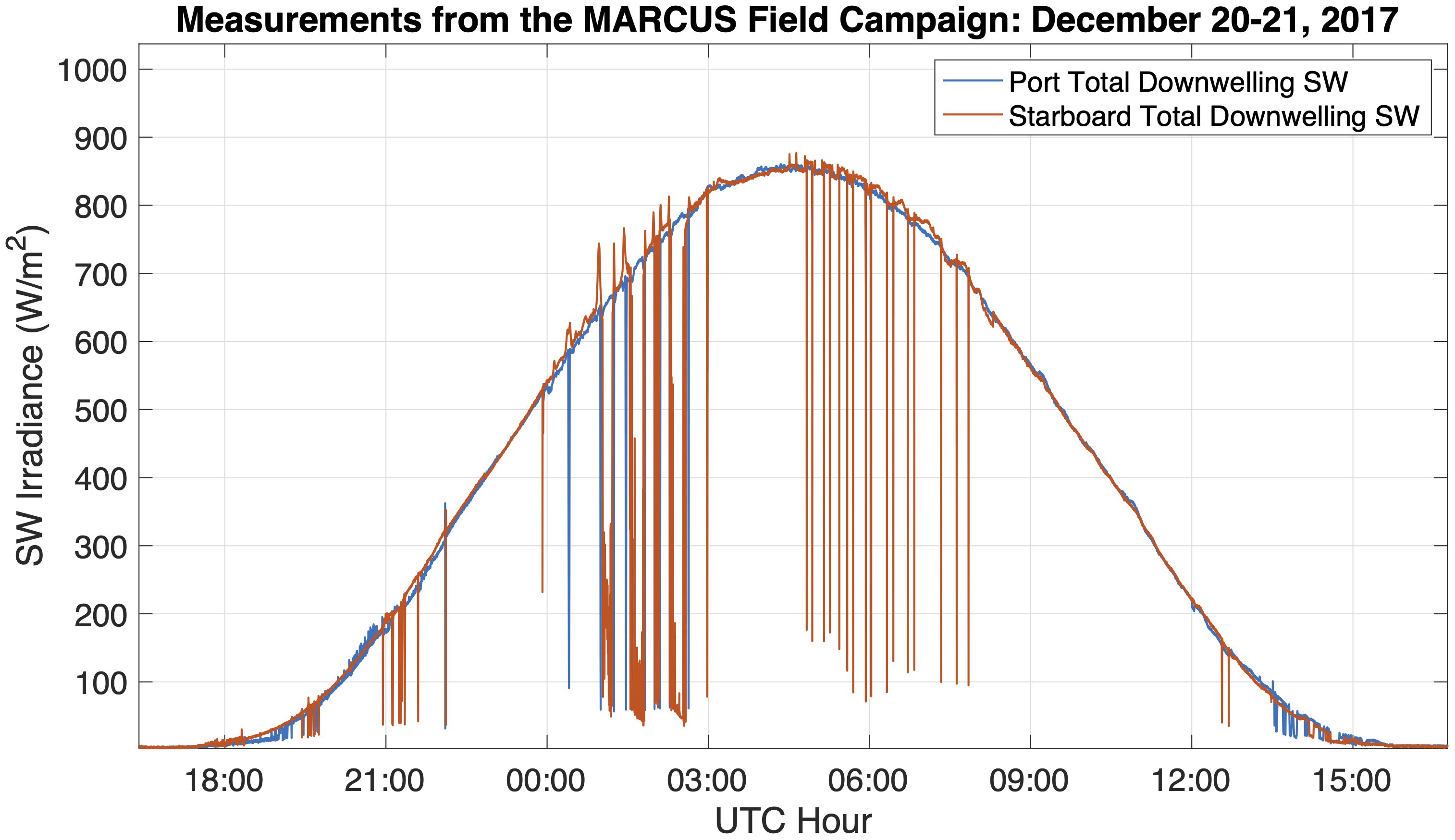
Figure 8 An example of redundant radiometer systems placed on the port and starboard sides of a ship in the Southern Ocean during the MARCUS field campaign. The dips in the data show shading from ship structures at different times on either side of the ship. The measurements have been tilt-corrected using the method described in Section 3.2.

However, including multiple instruments may be limited by cost and space constraints. And redundant measurements will not solve all problems. For example, errors due to platform motion will affect both sensors and thus will be difficult to identify through intercomparisons.

8.4.2 Automated tests

Basic automated limit checks can be applied to the data in order to identify obvious outliers. Long and Shi (2008) list tests for the most commonly observed variables. It should be noted, however, that their defined ranges assume that most of the data is good and errors are outside the statistical range of expected variability, however, many errors produce data within the normal range (e.g. Cox et al., 2021).

In general, these tests set limits based on physically possible limits and climatologies of data for a given site. For SW, this requires taking into account the diurnal cycle of the data, for example, as described in Equation 4 with an estimate of a physically possible maximum.

$\begin{array}{ll}S{W}_{max} = S_a\ast 1.5\ast {\mu }_o^{1.2}+100,& (4)\end{array}$

where $S_a$ is the solar constant adjusted for Earth-Sun distance (or the calculated solar irradiance incident on the top of the atmosphere), and ${\mu }_o^{}$ is the cosine of the solar zenith angle.

Equations also exist for calculating clear sky irradiance (Section 8.5), which can be used as a visual check on whether SW data match estimated clear sky curves for times which appear to not be impacted by clouds.

For downwelling LW irradiance, automated QC can be applied by comparing LW observations to the calculation of emission using the Stefan-Boltzmann equation and coincident measurements of temperature, e.g., $L_{eff} = \sigma T^4$. McArthur (2005) reports that the LW irradiance should generally be smaller than the effective irradiance calculation, except in cases of strong temperature inversion over a cold surface or in isothermal fog, and that assuming a surface emissivity of 0.75 as a lower bound can give a lower limit for downwelling LW irradiance. Alternatively a clear sky downwelling LW estimate can be used as a lower limit for evaluating measured downwelling LW as long as it is sufficiently relevant to the conditions at a given time and location. See Section 8.5 for methods to calculate clear sky.

Several codes that automate qc of radiation measurements are listed on the BSRN website at https://bsrn.awi.de/software/other-qc-software/. These tests and codes have been developed for land-based measurements, however, and platforms that change their location or orientation as many ocean-based platforms do may require different tests. Thus, we recommend that automated tests for ocean-based platforms be developed and open-source codes provided to the community.

8.4.3 Manual QC

The automated tests in the previous section may catch large errors, but are not a substitute for manual quality control. A well-trained data manager can often remove the impacts from shading (Figure 8), birds (Figure 9), or other field conditions.

Figure 9

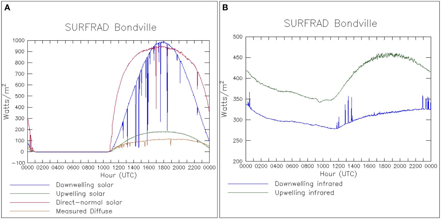
Figure 9 Spikes are seen in the SW (A) and LW (B) irradiance due to birds flying near or landing on sensors at the Bondville station in the land-based SURFRAD network on May, 7, 2018. Downward spikes are seen in the downwelling pyranometer measurements [(A), blue line] due to birds blocking sunlight from reaching the sensor. Upward spikes in the downwelling LW measurements [(B), blue line] are seen due to the extra heat that the pyrgeometers detect from the body heat of the birds.

A final note for this section is that recording raw radiometer signals, including thermopile voltages, as well as case and dome temperatures, is valuable for quality assessment and control as well as allowing radiation to be recomputed if calibration changes or in case of instrument malfunction. Higher-temporal resolution data can also be helpful for manual quality control, as impacts of short-term disturbances can sometimes be seen in high-temporal resolution data. These data are also useful to isolate problem areas such as understanding whether problems are in the instruments, datalogging systems, etc. For example, when desiccant fails condensation may occur inside an instrument’s dome. This is not apparent with PIRs as the dome is not transparent to the eye, but errors can manifest as a sudden large change in flux a few hours after sunrise when solar warming evaporates the moisture.

8.5 Calculating clear-sky irradiance

Estimates of clear sky irradiance at a given time and location can help with both quality control and scientific interpretation of the data. A number of methodologies exist to calculate clear sky irradiance, particularly for SW; some discussion of their accuracies is given here to help direct the community towards the most useful models.

The first factor that is needed in most clear sky SW irradiance methods is an accurate calculation of the solar position for a given place and time (e.g., ephemeris calculations of solar zenith angle, elevation angle, and azimuth angle). As a convenience to direct the community to useful calculations, we suggest a few models that are of known accuracy, though this is not meant to be exhaustive. Michalsky (1988) gives a model with stated azimuth and zenith angle accuracy of 0.01°, and includes printed fortran code in the appendix. An implementation of a solar position algorithm in C (https://midcdmz.nrel.gov/spa/), with an accuracy of 0.0003°, is described by Reda and Andreas (2004). This algorithm is widely used, and has been implemented in commonly used tools like pvlib available for Matlab and Python (Holmgren et al., 2018; https://pvpmc.sandia.gov/applications/pv_lib-toolbox/) and the Python library pysolar (Stafford et al., 2021; https://pysolar.readthedocs.io/en/latest/).

With an accurate calculation of solar position, SW clear sky irradiance can be estimated using an empirical approach such as that of Long and Ackerman (2000), which fits a curve to points that are identified as clear, or by modeling the clear sky. An advantage of the empirical approach is that estimates of other atmospheric parameters like aerosol loading and water vapor concentrations are not needed. Empirical fits to the data will also remove some measurement errors when creating ratios or differences between measured and calculated clear sky irradiance. For example, if a pyranometer has a calibration bias, the clear sky curve will have that same bias so it will be reduced in calculations of the transmissivity. However, the Long and Ackerman (2000) algorithm requires measurements of diffuse and total irradiance to identify clear skies, and the impact of sensor motion must be calculated, so it is not applicable to all measurements.

Care must be taken when applying a clear-sky fit function found with data from a pyranometer to measurements made by another model of pyranometer, because the fit may be affected by instrument characteristics, such as the cosine response. Furthermore, the clear sky fit found in a certain surface condition may not be suitable if the surface albedo changes, as could be the case for measurements taken in polar regions. The Long and Ackerman (2000) method handles these challenges by fitting to as many clear sky days as possible within the time series and interpolating the fit parameters between those clear days. This can give more inaccurate results when a site has frequent cloudy skies as there will be fewer clear sky fits.

The SW irradiance can be modeled using physical radiative transfer calculations or with a combination of radiative transfer and parameterized elements. All models require some characterization of inputs like aerosol, water vapor, and surface albedo. Sun et al. (2019) performed a robust comparison of 75 different clear sky models against 75 high quality ground-based land stations representing five climate regimes (i.e., equatorial, arid, temperate, cold, polar) using input data from the MERRA-2 reanalysis data. The MAC2 (Davies and McKay, 1982) and REST2v5 (Gueymard, 2008) models stood out as the top performing models globally, though some models performed better in particular climate regimes. Most of these models were coded using the R computer language by the authors, and are available online (Bright and Sun, 2018).

Clear-sky, surface LW estimates are based on the emissivity of the atmosphere. If temperature and humidity profiles of the atmosphere are available for a given location and time, clear-sky estimates can be calculated via radiative transfer models. There are also a number of parameterized models that use measurements of the ambient air temperature and humidity to approximate the emission of the atmospheric profile. These parameterizations generally take the form of Equation 5, where an effective clear-sky broadband emissivity (${\epsilon }_c$) is estimated assuming that the atmosphere can be treated as a single slab:

$\begin{array}{ll}L{W}_c = {\epsilon }_c\sigma T_a^4& \text{(5),}\end{array}$

where $L{W}_c$ is the clear sky downwelling surface LW, ${\epsilon }_c$ is an effective clear-sky broadband emissivity, $\sigma$ is the Stephan-Boltzman constant, and $T_a$ is the ambient air temperature in K.

The challenging piece of this equation is estimating the effective clear-sky emissivity, and a number of models exist to make that calculation. These models are based on surface parameters (like air temperature, water vapor partial pressure) or bulk quantities, such as integrated water vapor, or a combination thereof. Flerchinger et al. (2009) compare 13 algorithms at 21 sites and find that the Dilley and O’Brien (1998), Prata (1996), and Ångström (1915) algorithms calculate clear sky the most accurately. Guo et al. (2019) compare 7 algorithms at 71 different global sites and claim that Carmona et al. (2014) performs the best, but found that different methods worked better in different climate regions. Shakespeare and Roderick (2021) published a model that includes the ability to also constrain CO₂ concentrations and lapse rate to better tailor a clear sky estimate to a particular time and place.

Clear sky downwelling LW can also be estimated empirically using fits to the data. For example, Long and Turner (2008) use empirically identified clear sky periods and surface temperature and humidity measurements to estimate LW clear sky. As they discuss, because ~90% of the surface LW signal comes from the lowest 1 km of the atmosphere, an accurate surface clear sky LW calculation depends primarily on how well the near surface temperature and humidity profile is known. They base their estimates on the Brutsaert (1975) formula of where the effective clear-sky emissivity in Equation 5 is:

$\begin{array}{ll}{\epsilon }_c=C{(\frac{e}{T_a})}^{1/7}& (6)\end{array}$

In Equation 6, $e$ is the vapor pressure in hPa, and C is the effective temperature/humidity lapse rate coefficient which Brutsaert (1975) calculated to be 1.24 for a standard atmosphere. Long and Turner (2008) scale this estimate to identified clear periods. This identification of clear sky intervals is one of the challenging pieces: during the day this problem can be solved by exploiting the SW irradiance data, while at night the method proposed by Marty and Philipona (2000), based on LW irradiance, air temperature and humidity measurements, may be applied.

Another empirically derived method is given in the appendix of Fairall et al. (2008), based on a number of ship cruises in the Pacific Ocean, with over half the measurements taken near the equator. A fit based on latitude and surface humidity is given in Equation 7, though an additional version that includes the integrated water vapor as a dependent variable is also given in the reference. This equation can also be adjusted to fit data from a particular field campaign.

$\begin{array}{ll}{\epsilon }_{c }= 0.52+\frac{0.13}{60}abs(lat) +(0.82 - \frac{0.03}{60}abs(lat))\sqrt{q_a} & (7)\end{array}$

where q_a is the specific humidity in g/kg, and $lat$ is latitude.

In future work, we recommend specific testing for the best clear sky models for ocean measurements at different latitudes, in order to find site-specific clear sky models based on the available atmospheric parameters.

9 Best practices for calibrating sensors

To better unify the land and ocean communities, we recommend the adoption of BSRN calibration practices by the ocean community. World reference standards for surface radiation measurements are defined and maintained by the WMO (WMO, 2018). Additionally, some calibration standards for radiometers have been developed by the International Organization for Standardization (ISO) and ASTM International. For example, the ISO, 9846 (1993) calibration standard for SW pyranometers describes outdoor calibration methodologies used by major calibration centers used by BSRN stations. There is no similar industry standard for pyrgeometer calibrations, but the BSRN does describe pyrgeometer calibration methodologies for the network, and has a working group that is actively working on improving pyrgeometer calibrations. To ensure consistency with other platforms, SW pyranometers should be calibrated against a reference traceable to the WRR, and LW pyrgeometers should be calibrated against a reference traceable to the World Infrared Standard Group (WISG).

Additional details of calibrations may need to be tailored to the practicalities of ocean deployments and warrant further discussion. At the time this document was written, BSRN manual version 2 (McArthur, 2005) is the latest published version, though work on the third version of the manual is underway and the calibration recommendations will be updated, making this an ideal time to come to consensus between the ocean and land communities on needed calibration standards. We recommend that the ocean-based community contribute to and adopt the calibration standards written in the next BSRN manual.

In addition to standardizing practices, a major recommendation from the 2020 OBPS Surface Radiation Community Working Group report (Cronin et al., 2021) was to develop plans to expand land-based calibration facilities to also calibrate ocean-based networks of sensors. Additionally, it was recommended to create and maintain a list of calibration centers who can uniformly calibrate instrumentation. As many ocean programs do not have a high volume of radiometers, this could help unify and ensure consistent quality across networks without requiring substantial new investment by individual groups.

Another recommendation is to compare instruments calibrated at different centers, for example, sending the same instrument to multiple places to be calibrated as a check on how consistent the calibration methods are between sites and individual calibration events.

Finally, when possible end-to-end calibration of instruments, datalogging, and software systems including all signal conditioning and related hardware and software is recommended to check calibration of the complete system.

It is likely that the uncertainties in ocean radiation observations in the field will be significantly greater than those derived from laboratory calibration, thus there is a need for quantification of these errors through intercomparison experiments as discussed more in the next section.

10 Need for intercomparison experiments and future research

A critical step in building a unified network between land and ocean and over multiple ocean platforms is to establish the comparability of the sensors as deployed in the field. Past studies have shown the importance of intercomparisons to quantify and understand the impact of differences in set up, electronics, calibrations, etc (e.g., Fairall et al., 1998; Joseph et al., 2022). Interoperability experiments and other targeted studies to identify best practices and quantify uncertainties associated with various options are thus recommended to reach higher accuracies and synthesis between communities and measurement networks. The well-established OceanSITES network of time series stations provide ready opportunities for these intercomparison field tests. We recommend that field intercomparisons against OceanSITES stations and other platforms be performed whenever possible to test the interoperability of different platforms for measuring a given essential ocean or climate variable. Recommendations for areas with a need for future research or community consensus in order to determine best practices or quantify the uncertainties associated with various options are detailed throughout the paper. We collect them here in Table 4 for ease of reference.

Table 4

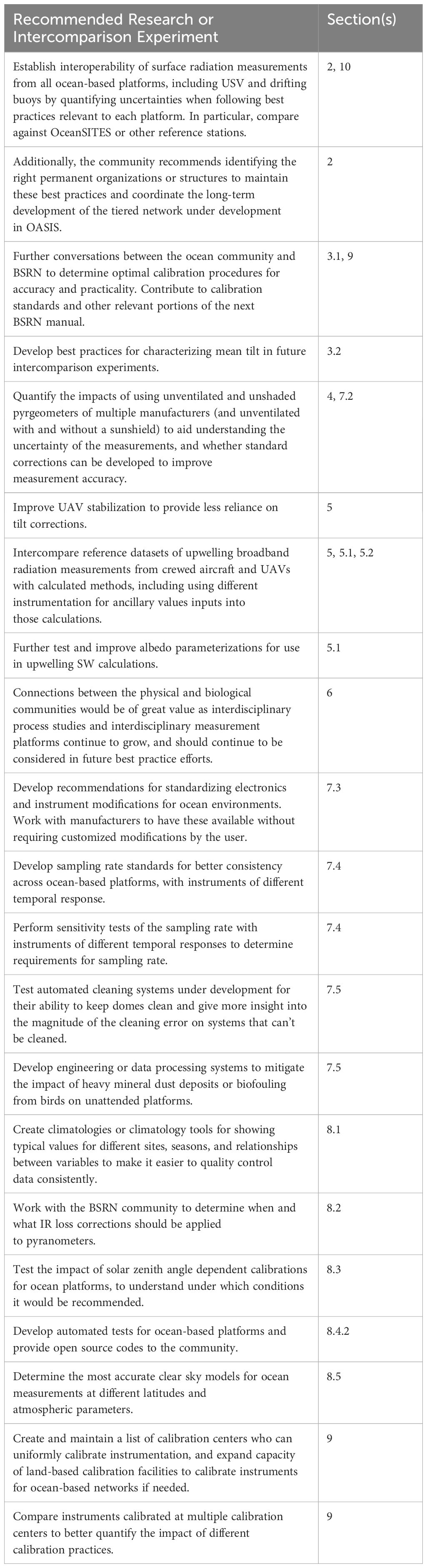
Table 4 Summary of recommended future experiments and research.

11 Summary of recommendations

For ease of reference, the best practice recommendations described in this article are summarized here in Table 5. The sections that describe these recommendations are also listed in the table, and the recommendations can be found in bold throughout the article.

Table 5

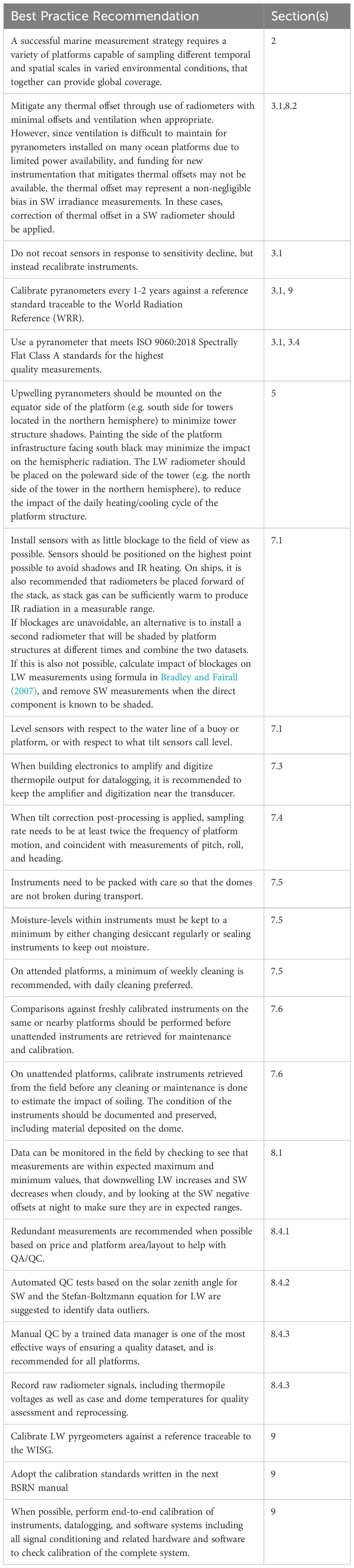
Table 5 Summary of best practice recommendations from throughout the paper.

12 Conclusion

A number of standards for surface radiation measurements have been created over the years within different communities. For example, recommendations were created for ship-based measurements (Bradley and Fairall, 2007). The BSRN created best practices for reducing uncertainties in measurements over land (McArthur, 2005; WMO, 2018). And the solar energy industry has created instrument and calibration standards focused on shortwave instrumentation (e.g., ISO, 9846, 1993; ISO, 9060:2018, 2018). In light of new technologies, such as improved SW and LW radiometers and new platforms like UAVs and USVs, and in light of new scientific objectives, such as OASIS and expanding the BSRN to include ocean-based measurements, additional efforts are needed to determine best practices for ocean-based platforms. This document was put together by bringing together experts from land, ocean, and aircraft-based radiometer measurements to develop a more unified set of best practices for SW and LW radiation measurements for oceanic platforms.

Standards that can be recommended based on current knowledge were described herein as well as a list of high priority needs for the community to determine through new experiments or discussions amongst various stakeholders.

While it is not possible to achieve the same measurement accuracy on all platforms, measurements from different platforms can be used more broadly when uncertainties are quantified. There is a need for more spatial coverage of the surface radiation budget. Thus, these best practices are not meant to restrict additional measurements when all these best practices can’t be met, but rather to be a motivator for establishing the level of interoperability between platforms for a tiered network approach for developing a broader global network. Existing high-quality measurements like BSRN and OceanSITES stations can form the backbone of an expanding network. When uncertainties are quantified for other platforms and practices through intercomparison experiments at these stations, the global network can be better tied together with a fuller understanding of the strengths and limitations of these measurements.

We hope this review of best practices for observing surface radiation sets the stage for this growing tiered network of ocean-based instrumentation that can seamlessly connect into the land-based network for broader scientific endeavors including studies of air-sea interactions and long-term climate reference networks.

Data availability statement

The original contributions presented in the study are included in the article/Supplementary Material. Further inquiries can be directed to the corresponding author.

Author contributions

LR: Writing – original draft, Writing – review & editing, Methodology, Visualization, Conceptualization. MC: Conceptualization, Project administration, Writing – review & editing, Methodology, Supervision. RA: Writing – review & editing. NA: Writing – review & editing. JA: Visualization, Writing – review & editing. KB: Writing – review & editing. PB: Visualization, Writing – review & editing, Methodology. RB: Writing – review & editing. AB: Writing – review & editing, Methodology. KC: Writing – review & editing. CC: Methodology, Visualization, Writing – review & editing. AD: Writing – review & editing, Supervision, Methodology, Visualization. JE: Writing – review & editing, Methodology. CF: Methodology, Visualization, Writing – review & editing. JF: Writing – review & editing, Methodology. KG: Writing – review & editing, Methodology. MG: Writing – review & editing, Methodology. VH: Writing – review & editing. KJ: Writing – review & editing, Methodology. CL: Methodology, Writing – review & editing, Conceptualization. FM: Writing – review & editing. DM: Writing – review & editing, Methodology, Supervision. MO: Writing – review & editing. SP: Writing – review & editing, Visualization, Methodology. KR: Writing – review & editing. DR: Writing – review & editing, Visualization, Methodology. NS: Writing – review & editing. SS: Writing – review & editing, Methodology. SS: Writing – review & editing. AT: Methodology, Writing – review & editing. RV: Supervision, Writing – review & editing, Conceptualization. ET: Writing – review & editing, Methodology. RV: Writing – review & editing. VV: Writing – review & editing. KW: Methodology, Writing – review & editing, Writing – original draft. RW: Methodology, Writing – review & editing, Conceptualization, Visualization. CZ: Writing – review & editing, Methodology. DZ: Writing – review & editing, Methodology.

Funding

The author(s) declare financial support was received for the research, authorship, and/or publication of this article. Authors were funded by NOAA (LR, MC, NA, KC, CC, RW, KWB) including NOAA’s Global Ocean Monitoring and Observing Program (FundRef https://doi.org/10.13039/100018302) and NOAA cooperative agreements NA17OAR4320101 and NA22OAR4320151, the US Department of Energy Atmospheric Radiation Measurement Facility (LR), Office of Naval Research, US National Science Foundation’s Oceanographic Instrumentation and Technical Services Program (SRS), EU’s Horizon 2020 research and innovation programme under Grant Agreement 821001 (SOCHIC) & 951842 (GROOM II) for SS, and NASA (JF). The Lampedusa Observatory was supported by the Marine Hazard (PON03PE_00203_1) project, funded by the Italian Ministry for University and Research. The W1M3A research facility was partly supported by EMSO-ERIC through the national Joint Research Unit funded by the Italian Ministry for University and Research. We acknowledge funding provided by the Scientific Committee on Oceanic Research (SCOR) and from a grant to SCOR from the U.S. National Science Foundation (OCE-1840868 and OCE-1743430) to support SCOR Working Group #162 (OASIS and OOI) activities.

Acknowledgments

These best practices were developed from workshops held at the Ocean Best Practices Systems meetings in 2020 and 2021, led by the Observing Air-Sea Interactions Strategy and the BSRN Ocean Working Group. They have been endorsed by the OceanSITES network, and are in the process of being endorsed by the Global Ocean Observing System and the Global Climate Observing System steering panels. This is NOAA PMEL Publication # 5572.

Conflict of interest

Author David Rutan is employed by Adnet Systems United States, Matteo Ottaviani by Terra Research Inc, and Christian Lanconelli by Unisystems SA.

The remaining authors declare that the research was conducted in the absence of any commercial or financial relationships that could be construed as a potential conflict of interest.

The author(s) declared that they were an editorial board member of Frontiers, at the time of submission. This had no impact on the peer review process and the final decision.

Publisher’s note

All claims expressed in this article are solely those of the authors and do not necessarily represent those of their affiliated organizations, or those of the publisher, the editors and the reviewers. Any product that may be evaluated in this article, or claim that may be made by its manufacturer, is not guaranteed or endorsed by the publisher.

Supplementary material

The Supplementary Material for this article can be found online at: https://www.frontiersin.org/articles/10.3389/fmars.2024.1359149/full#supplementary-material

References

Ångström A. (1915). A study of the radiation of the atmosphere, Smithson. Misc. Collect. 65, 1–159.

Google Scholar

Amber I., O’Donovan T. S. (2018). Natural convection induced by the absorption of solar radiation: A review. Renewable Sustain. Energy Rev. 82, 3526–3545. doi: 10.1016/j.rser.2017.10.106

CrossRef Full Text | Google Scholar

Badosa J., Wood J., Blanc P., Long C. N., Vuilleumier L., Demengel D., et al. (2014). Solar irradiances measured using SPN1 radiometers: uncertainties and clues for development. Atmos. Meas. Tech. 7, 4267–4283. doi: 10.5194/amt-7-4267-2014

CrossRef Full Text | Google Scholar

Blondeau-Patissier D., Gower J. F., Dekker A. G., Phinn S. R., Brando V. E. (2014). A review of ocean color remote sensing methods and statistical techniques for the detection, mapping and analysis of phytoplankton blooms in coastal and open oceans. Prog. Oceanogr. 123, 123–144. doi: 10.1016/j.pocean.2013.12.008

CrossRef Full Text | Google Scholar

Bradley E. F., Fairall C. W. (2007). A guide to making climate quality meteorological and flux measurements at sea (Boulder, CO: NOAA Technical Memorandum OAR PSD-311), 109. Available at: https://downloads.psl.noaa.gov/BLO/Air-Sea/wcrp_wgsf/flux_handbook/fluxhandbook_NOAA-TECH%20PSD-311v3.pdf.

Google Scholar

Bright J. M., Sun X. (2018). A library of clear-sky irradiance models coded in R. Available online at: https://jamiembright.github.io/clear-sky-models/.

Google Scholar

Brutsaert W. (1975). On a derivable formula for long-wave radiation from clear skies. Water Resour. Res. 11 (5), 742–744. doi: 10.1029/WR011i005p00742

CrossRef Full Text | Google Scholar

BSRN Operation manual v3. Available online at: www.bsrn.awi.de/fileadmin/user_upload/bsrn.awi.de/Publications/McArthur.pdf.

Google Scholar

Bucholtz A., Bluth R. T., Kelly B., Taylor S., Batson K., Sarto A. W., et al. (2008). The stabilized radiometer platform (STRAP) - an actively stabilized horizontally level platform for improved aircraft irradiance measurements. J. Atmos. Oceanic Tech. 25, 2161–2175. doi: 10.1175/2008JTECHA1085.1

CrossRef Full Text | Google Scholar

Calmer R., de Boer G., Hamilton J., Lawrence D., Webster M. A., Wright N., et al. (2023). Relationships between summertime surface albedo and melt pond fraction in the central Arctic Ocean: The aggregate scale of albedo obtained on the MOSAiC floe. Elementa: Sci. Anthropocene 11, 1. doi: 10.1525/elementa.2023.00001

CrossRef Full Text | Google Scholar

Carmona F., Rivas R., Caselles C. (2014). Estimation of daytime downward longwave radiation under clear and cloudy skies conditions over a sub-humid region. Theor. Appl. Climatol. 115, 281–295. doi: 10.1007/s00704-013-0891-3

CrossRef Full Text | Google Scholar

Clough S. A., Shephard M. W., Mlawer E. J., Delamere J. S., Iacono M. J., Cady-Pereira K., et al. (2005). Atmospheric radiative transfer modeling: a summary of the AER codes. Journal of Quantitative Spectroscopy and Radiative Transfer. 91(2), 233–244. doi: 10.1016/j.jqsrt.2004.05.058

CrossRef Full Text | Google Scholar

Colbo K., Weller R. A. (2009). Accuracy of the IMET sensor package in the subtropics. J. Atmos. Oceanic Tech. 26, 1867–1890. doi: 10.1175/2009JTECHO667.1

CrossRef Full Text | Google Scholar

Cox C. J., Gallagher M. R., Shupe M. D., Persson P. O. G., Solomon A., Fairall C. W., et al. (2023). Continuous observations of the surface energy budget and meteorology over the Arctic sea ice during MOSAiC. Sci. Data 10, 519. doi: 10.1038/s41597-023-02415-5

PubMed Abstract | CrossRef Full Text | Google Scholar

Cox C. J., Morris S. M., Uttal T., Burgener R., Hall E., Kutchenreiter M., et al. (2021). The De-Icing Comparison Experiment (D-ICE): a study of broadband radiometric measurements under icing conditions in the Arctic. Atmos. Meas. Tech. 14, 1205–1224. doi: 10.5194/amt-14-1205-2021

CrossRef Full Text | Google Scholar

Cronin M. F., Bond N. A., Fairall C. W., Weller R. A. (2006). Surface cloud forcing in the east Pacific stratus deck/cold tongue/ITCZ complex. J. Climate 19, 392–409. doi: 10.1175/JCLI3620.1

CrossRef Full Text | Google Scholar

Cronin M. F., Gentemann C. L., Edson J., Ueki I., Bourassa M., Brown S., et al. (2019). Air-sea fluxes with a focus on heat and momentum. Front. Mar. Sci. 6. doi: 10.3389/fmars.2019.00430

CrossRef Full Text | Google Scholar

Cronin M. F., Pelland N. A., Emerson S. R., Crawford W. R. (2015). Estimating diffusivity from the mixed layer heat and salt balances in the North Pacific. J. Geophys. Res. Oceans 120, 7346–7362. doi: 10.1002/2017GL076805

CrossRef Full Text | Google Scholar

Cronin M. F., Riihimaki L., Guerra M. T., Thompson E., Anderson N., Berk P., et al. (2021). “Surface radiation community working group report,” in Evolving and Sustaining Ocean Best Practices Workshop IV, , 18; 21-25 & 30 Sep 2020, vol. 2 . Eds. Simpson P., Pearlman F., Pearlman J. (UNESCO, Paris, France), 98–111. IOC Workshop Report No. 294. doi: 10.25607/OBP-1036

CrossRef Full Text | Google Scholar

Cronin M. F., Swart S., Marandino C. A., Anderson C., Browne P., Chen S., et al. (2023). Developing an Observing Air–Sea Interactions Strategy (OASIS) for the global ocean. ICES J. Mar. Sci. 80, 367–373. doi: 10.1093/icesjms/fsac149

CrossRef Full Text | Google Scholar

Davies J., McKay D. (1982). Estimating solar irradiance and components. Solar Energy 29, 55–64. doi: 10.1016/0038-092X(82)90280-8

CrossRef Full Text | Google Scholar

Delta-T Devices Ltd. (2019). User Manual for the Sunshine Pyranometer type SPN1, SPN1-UM v4.2. Available at: https://delta-t.co.uk/wp-content/uploads/2019/06/SPN1_User_Manual_4.2.pdf (Accessed 13 December 2021).

Google Scholar

Dilley A. C., O’Brien D. M. (1998). Estimating downward clear skylong-wave irradiance at the surface from screen temperature and precipitable water. Q.J.R. Meteorol. Soc 124, 1391–1401. doi: 10.1002/qj.49712454903

CrossRef Full Text | Google Scholar

di Sarra A., Bommarito C., Anello F., Di Iorio T., Meloni D., Monteleone F., et al. (2019). Assessing the Quality of Shortwave and Longwave Irradiance Observations over the Ocean: One Year of High-Time-Resolution Measurements at the Lampedusa Oceanographic Observatory. J. Atmos. Oceanic Tech. 36, 2383–2400. doi: 10.1175/JTECH-D-19-0018.1

CrossRef Full Text | Google Scholar

Donlon C. J., Minnett P. J., Jessup A. T., Barton I., Emery W., Hook S., et al. (2014). Ship-borne thermal infrared radiometer systems, Experimental Methods in the Physical Sciences. Optical Radiometry Ocean Climate Meas. 47, 305–404. doi: 10.1016/B978-0-12-417011-7.00011-8

CrossRef Full Text | Google Scholar

Driemel A., Augustine J., Behrens K., Colle S., Cox C., Cuevas-Agulló E., et al. (2018). Baseline Surface Radiation Network (BSRN): structure and data description, (1992-2017). Earth Syst. Sci. Data 10, 1491–1501. doi: 10.5194/essd-10-1491-2018

CrossRef Full Text | Google Scholar

Dutton E. G., Michalsky J. J., Stoffel T., Forgan B. W., Hickey J., Nelson D. W., et al. (2001). Measurement of broadband diffuse solar irradiance using current commercial instrumentation with a correction for thermal offset errors. J. Atmos. Oceanic Tech. 18, 297–314. doi: 10.1175/1520-0426(2001)018%3C0297:MOBDSI%3E2.0.CO;2

CrossRef Full Text | Google Scholar

Enomoto T. (2007). Ocean surface albedo in AFES. JAMSTEC Rep. Res. Dev. 6, 21–30. doi: 10.5918/jamstecr.6.21

CrossRef Full Text | Google Scholar

Fairall C. W., Bradley E. F., Godfrey J. S., Wick G. A., Edson J. B., Young G. S. (1996). Cool-skin and warm-layer effects on sea surface temperature. J. Geophys. Res. 101, 1295–1308. doi: 10.1029/95JC03190

CrossRef Full Text | Google Scholar

Fairall C. W., Bradley E. F., Hare J. E., Grachev A. A., Edson J. B. (2003). Bulk parameterization of air-sea fluxes: Updates and verification for the COARE algorithm. J. Climate 16, 571–591. doi: 10.1175/1520-0442(2003)016<0571:BPOASF>2.0.CO;2

CrossRef Full Text | Google Scholar

Fairall C. W., Persson O. P. G., Payne R. E., Bradley E. F. (1998). A new look at calibration and use of Eppley precision infrared radiometers. J. Atmos. Oceanic Tech. 15, 1230–1243. doi: 10.1175/1520-0426(1998)015<1229:ANLACA>2.0.CO;2

CrossRef Full Text | Google Scholar

Fairall C. W., Uttal T., Hazen D., Hare J., Cronin M. F., Bond N., et al. (2008). Observations of Cloud, Radiation, and Surface Forcing in the Equatorial Eastern Pacific. J. Climate 21, 655–673. doi: 10.1175/2007JCLI1757.1

CrossRef Full Text | Google Scholar

Field C. B., Behrenfeld M. J., Randerson J. T., Falkowski P. (1998). Primary production of the biosphere: Integrating terrestrial and oceanic components. Science 281, 237–240. doi: 10.1126/science.281.5374.237

PubMed Abstract | CrossRef Full Text | Google Scholar

Flerchinger G. N., Xaio W., Marks D., Sauer T. J., Yu Q. (2009). Comparison of algorithms for incoming atmospheric long-wave radiation. Water Resour. Res. 45, W03423. doi: 10.1029/2008WR007394

CrossRef Full Text | Google Scholar

Foltz G. R., Evan A. T., Freitag H. P., Brown S., McPhaden M. J. (2013a). Dust accumulation biases in PIRATA shortwave radiation records. J. Atmos. Oceanic Tech. 30, 1414–1432. doi: 10.1175/JTECH-D-12-00169.1

CrossRef Full Text | Google Scholar

Foltz G. R., Schmid C., Lumpkin R. (2013b). Seasonal cycle of the mixed layer heat budget in the Northeastern Tropical Atlantic Ocean. J. Climate 26, 8169–8188. doi: 10.1175/JCLI-D-13-00037.1

CrossRef Full Text | Google Scholar

Frouin R., Ramon D., Boss E., Jolivet D., Compiègne M., Tan J., et al. (2018). Satellite radiation products for ocean biology and biogeochemistry: needs, state-of-the-art, gaps, development priorities, and opportunities. Front. Mar. Sci. 5. doi: 10.3389/fmars.2018.00003

CrossRef Full Text | Google Scholar

GCOS (2021). The Status of the Global Climate Observing System 2021: The GCOS Status Report (GCOS-240) (Geneva: WMO). Available at: https://gcos.wmo.int/en/publications/gcos-status-report-2021.

Google Scholar

GCOS (2022). The 2022 GCOS ECV Requirements (GCOS-245) (Geneva: WMO), 1–244. Available at: https://library.wmo.int/idurl/4/58111.

Google Scholar

Gentemann C. L., Scott J. P., Mazzini P. L. F., Pianca C., Akella S., Minnett P. J., et al. (2020). Saildrone: adaptively sampling the marine environment. Bull. Am. Meteorological Society 101, E744–E762. doi: 10.1175/BAMS-D-19-0015.1

CrossRef Full Text | Google Scholar

Geuder N., Quaschning V. (2006). Soiling of irradiation sensors and methods for soiling correction. Solar Energy 80, 1402–1409. doi: 10.1016/j.solener.2006.06.001

CrossRef Full Text | Google Scholar

Gueymard C. (2008). REST2: High-performance solar radiation model for cloudless-sky irradiance, illuminance, and photosynthetically active radiation: Validation with a benchmark dataset. Solar Energy 82, 272–285. doi: 10.1016/j.solener.2007.04.008

CrossRef Full Text | Google Scholar

Gueymard C. A., Myers D. R. (2009). Evaluation of conventional and high-performance routine solar radiation measurements for improved solar resource, climatological trends, and radiative modeling. Solar Energy 83, 171–185. doi: 10.1016/j.solener.2008.07.015

CrossRef Full Text | Google Scholar

Guo Y., Cheng J., Liang S. (2019). Comprehensive assessment of parameterization methods for estimating clear-sky surface downward longwave radiation. Theor. Appl. Climatol. 135, 1045–1058. doi: 10.1007/s00704-018-2423-7

CrossRef Full Text | Google Scholar

Hogikyan A., Cronin M. F., Zhang D., Kato S. (2020). Uncertainty in net surface heat flux due to differences in commonly used albedo products. J. Climate 33, 303–315. doi: 10.1175/JCLI-D-18-0448.1

CrossRef Full Text | Google Scholar

Holmgren W., Hansen C., Mikofski M. (2018). pvlib Python: A python package for modeling solar energy systems. J. Open Source Software 3, 884. doi: 10.21105/joss.00884

CrossRef Full Text | Google Scholar

IOCCG (2014). Phytoplankton Functional Types from Space. Ed. Sathyendranath S. (Dartmouth, NS, Canada: International Ocean-Colour Coordinating Group (IOCCG), 154pp. Reports of the International Ocean-Colour Coordinating Group, No. 15. doi: 10.25607/OBP-106

CrossRef Full Text | Google Scholar

IOCCG Protocol Series (2019). “Protocols for satellite ocean colour data validation: in situ optical radiometry,” in IOCCG Ocean Optics and Biogeochemistry Protocols for Satellite Ocean Colour Sensor Validation, vol. 3.0 . Eds. Zibordi G., Voss K. J., Johnson B. C., Mueller J. L. (IOCCG, Dartmouth, NS, Canada). doi: 10.25607/OBP-691

CrossRef Full Text | Google Scholar

ISO, 9060:2018 (2018). Solar energy - Specification and classification of instruments for measuring hemispherical solar and direct solar radiation. Available at: https://www.iso.org/standard/67464.html.

Google Scholar

ISO, 9846 (1993). Calibration of a pyranometer using a pyrheliometer. Available at: https://www.iso.org/standard/17724.html.

Google Scholar

Jin Z., Charlock T. P., Rutledge K., Stamnes K., Wang Y. (2006). Analytical solution of radiative transfer in the coupled atmosphere-ocean system with a rough surface. App. Opt. 45, 7443–7455. doi: 10.1364/AO.45.007443

CrossRef Full Text | Google Scholar

Jin Z., Charlock T. P., Smith W. L. Jr., Rutledge K. (2004). A parameterization of ocean surface albedo. Geophys. Res. Lett. 31, L223013. doi: 10.1029/2004GL021180

CrossRef Full Text | Google Scholar

Jin Z., Ottaviani M., Sikand M. (2023). Modeling sea ice albedo and transmittance measurements with a fully-coupled radiative transfer model. Opt. Express 31, 21128–21152. doi: 10.1364/OE.491306

PubMed Abstract | CrossRef Full Text | Google Scholar

Joseph K. J., Tandon A., Venkatesan R., Farrar J. T., Weller R. A. (2022). Longwave radiation corrections for the OMNI buoy network. J. Atmos. Oceanic Tech. 39, 271–282. doi: 10.1175/JTECH-D-21-0069.1

CrossRef Full Text | Google Scholar

Kassianov E., Long C. N., Ovtchinnikov M. (2005). Cloud sky cover versus cloud fraction: Whole-sky simulations and observations. J. Appl. Meteor. 44, 86–98. doi: 10.1175/JAM-2184.1

CrossRef Full Text | Google Scholar

Lee C. M., DeGrandpre M., Guthrie J., Hill V., Kwok R., Morison J., et al. (2022). Emerging technologies and approaches for in situ, autonomous observing in the Arctic. Oceanogr. 35, 210–221. doi: 10.5670/oceanog.2022.127

CrossRef Full Text | Google Scholar

Long C. N., Ackerman T. P. (2000). Identification of clear skies from broadband pyranometer measurements and calculation of downwelling shortwave cloud effects. J. Geophys. Res. 105, 15609–15626. doi: 10.1029/2000JD900077

CrossRef Full Text | Google Scholar

Long C. N., Ackerman T. P., Gaustad K. L., Cole J. N. S. (2006). Estimation of fractional sky cover from broadband shortwave radiometer measurements. J. Geophys. Res. 111, D11204. doi: 10.1029/2005JD006475

CrossRef Full Text | Google Scholar

Long C. N., Bucholtz. A., Jonsson H., Schmid B., Vogelmann A. M., Wood J. (2010). A method of correcting for tilt from horizontal in downwelling shortwave irradiance measurements on moving platforms. Open Atmospheric Sci. J. 4, 78–87. doi: 10.2174/1874282301004010078

CrossRef Full Text | Google Scholar

Long C. N., Shi Y. (2008). An automated quality assessment and control algorithm for surface radiation measurements. Open Atmospheric Sci. J. 2, 23–37. doi: 10.2174/1874282300802010023

CrossRef Full Text | Google Scholar

Long C. N., Turner D. D. (2008). A method for continuous estimation of clear-sky downwelling longwave radiative flux developed using ARM surface measurements. J. Geophys. Res. 113, D18206. doi: 10.1029/2008JD009936

CrossRef Full Text | Google Scholar

Lotliker A. A., Omand M. M., Lucas A. J., Laney S. R., Mahadevan A., Ravichandran M. (2016). Penetrative radiative flux in the Bay of Bengal. Oceanogr. 29, 214–221. doi: 10.5670/oceanog.2016.53

CrossRef Full Text | Google Scholar

MacWhorter M. A., Weller R. A. (1991). Error in measurements of incoming shortwave radiation made from ships and buoys. J. Atmos. Oceanic Tech. 8, 108–117. doi: 10.1175/1520-0426(1991)008<0108:EIMOIS>2.0.CO;2

CrossRef Full Text | Google Scholar

Marty C., Philipona R. (2000). The clear-sky index to separate clear‐sky from cloudy-sky situations in climate research. Geophysical Research Letters 27 (17), 2649–2652. doi: 10.1029/2000GL011743

CrossRef Full Text | Google Scholar

Marullo S., Minnett P. J., Santoleri R., Tonani M. (2016). The diurnal cycle of sea-surface temperature and estimation of the heat budget of the Mediterranean Sea. J. Geophys. Res. Oceans 121, 8351–8367. doi: 10.1002/2016JC012192

CrossRef Full Text | Google Scholar

McArthur L. J. B. (2005). World Climate Research Programme-Baseline Surface Radiation Network (BSRN)-Operations Manual Version 2.1 (Downsview, Ontario, CANADA: Experimental Studies Division, Atmospheric Environment Service). Available at: www.bsrn.awi.de/fileadmin/user_upload/bsrn.awi.de/Publications/McArthur.pdf.

Google Scholar

McCree K. J. (1972). Test of current definitions of photosynthetically active radiation against leaf photosynthesis data. Agric. Meteorol. 10, 443–453. doi: 10.1016/0002-1571(72)90045-3

CrossRef Full Text | Google Scholar

McFarquhar G. M., Bretherton C. S., Marchand R., Protat A., DeMott P. J., Alexander S. P., et al. (2021). Observations of clouds, aerosols, precipitation, and surface radiation over the southern ocean: an overview of CAPRICORN, MARCUS, MICRE, and SOCRATES. Bull. Am. Meteorological Society 102, E894–E928. doi: 10.1175/BAMS-D-20-0132.1

CrossRef Full Text | Google Scholar

Meloni D., Di Biagio C., di Sarra A., Monteleone F., Pace G., Sferlazzo D. M. (2012). Accounting for the solar radiation influence on downward longwave irradiance measurements by pyrgeometers. J. Atmos. Ocean. Technol. 29, 1629–1643. doi: 10.1175/JTECH-D-11-00216.1

CrossRef Full Text | Google Scholar

Michalsky J. J. (1988). The Astronomical Almanac’s algorithm for approximate solar position, (1950–2050). Solar Energy 40, 227–235. doi: 10.1016/0038-092X(88)90045-X

CrossRef Full Text | Google Scholar

Michalsky J. J., Harrison L. C., Berkheiser W. E. (1995). Cosine response characteristics of some radiometric and photometric sensors. Solar Energy 54, 397–402. doi: 10.1016/0038-092X(95)00017-L

CrossRef Full Text | Google Scholar

Mueller J. L., Morel A., Frouin R., Davis C., Arnone R., Carder K., et al. (2003). Ocean Optics Protocols For Satellite Ocean Color Sensor Validation, Revision 4, Volume III: Radiometric Measurements and Data Analysis Protocols (Greenbelt, MD: Goddard Space Flight Space Centre), 1–84. NASA/TM-2003-21621/Rev-Vol III. doi: 10.25607/OBP-62

CrossRef Full Text | Google Scholar

Myers D. R., Andreas R., Stoffel T., Reda I., Wilcox S., Gotseff P., et al. (2001). Radiometric Calibrations, Measurements, and Standards Development at NREL (Lakewood, CO: National Renewable Energy Laboratory). Available at: https://www.nrel.gov/docs/fy02osti/30964.pdf.

Google Scholar

Nicolaus M., Hudson S. R., Gerland S., Munderloh K. (2010). A modern concept for autonomous and continuous measurements of spectral albedo and transmittance of sea ice. Cold Regions Sci. Technol. 62, 14–28. doi: 10.1016/j.coldregions.2010.03.001

CrossRef Full Text | Google Scholar

Ohlmann J. C., Siegel D. A., Mobley C. D. (2000). Ocean radiant heating. Part I: Optical influences. J. Phys. Ocean. 30, 1883–1848. doi: 10.1175/1520-0485(2000)030<1833:ORHPIO>2.0.CO;2

CrossRef Full Text | Google Scholar

Ohmura A., Dutton E. G., Forgan B., Fröhlich C., Gilgen H., Hegner H., et al. (1998). Baseline surface radiation network (BSRN/WCRP): new precision radiometry for climate research. Bull. Am. Meteorological Society 79, 2115–2136. doi: 10.1175/1520-0477(1998)079<2115:BSRNBW>2.0.CO;2

CrossRef Full Text | Google Scholar

Owens W. B., Zilberman N., Johnson K. S., Claustre H., Scanderbeg M., Wijffels S., et al. (2022). OneArgo: a new paradigm for observing the global ocean. Mar. Technol. Soc. J. 56, 84–90. doi: 10.4031/MTSJ.56.3.8

CrossRef Full Text | Google Scholar

Paulson C. A., Simpson J. J. (1977). Irradiance measurements in the upper ocean. J. Phys. Oceanogr. 7, 952–956. doi: 10.1175/1520-0485(1977)007<0952:IMITUO>2.0.CO;2

CrossRef Full Text | Google Scholar

Payne R. E. (1972). Albedo of the sea surface. J. Atmospheric Sci. 29, 959–970. doi: 10.1175/1520-0469(1972)029<0959:AOTSS>2.0.CO;2

CrossRef Full Text | Google Scholar

Persson P. O. G., Fairall C. W., Andreas E. L., Guest P. S., Perovich D. K. (2002). Measurements near the Atmospheric Surface Flux Group tower at SHEBA: Near-surface conditions and surface energy budget. J. Geophys. Res.: Oceans 107, 8054. doi: 10.1029/2000JC000705

CrossRef Full Text | Google Scholar

Pinker R., Zhang B., Weller R., Chen W. (2018). Evaluating surface radiation fluxes observed from satellites in the Southeastern Pacific Ocean. Geophys. Res. Lett. 45, 2404–2412. doi: 10.1002/2017GL076805

CrossRef Full Text | Google Scholar

Prata A. J. (1996). A new long-wave formula for estimating downward clear-sky radiation at the surface. Q.J.R. Meteorol. Soc 122, 1127–1151. doi: 10.1002/qj.49712253306

CrossRef Full Text | Google Scholar

Qiu J. (2001). Broadband extinction method to determine atmospheric aerosol optical properties. Tellus B: Chem. Phys. Meteorol. 53, 72–82. doi: 10.3402/tellusb.v53i1.16540

CrossRef Full Text | Google Scholar

Reda I., Andreas A. (2004). Solar position algorithm for solar radiation applications. Solar Energy 76, 577–589. doi: 10.1016/j.solener.2003.12.003

CrossRef Full Text | Google Scholar

Reineman B. D., Lenain L., Statom N. M., Kendall Melville W. (2013). Development and testing of instrumentation for UAV-based flux measurements within terrestrial and marine atmospheric boundary layers. J. Atmos. Oceanic Technol. 30, 1295–1319. doi: 10.1175/JTECH-D-12-00176.1

CrossRef Full Text | Google Scholar

Reynolds R. M., Miller M. A., Bartholomew M. J. (2001). Design, operation, and calibration of a shipboard Fast-Rotating Shadowband Spectral Radiometer. J. Atmos. Ocean. Technol. 18, 200–214. doi: 10.1175/1520-0426(2001)018<0200:DOACOA>2.0.CO;2

CrossRef Full Text | Google Scholar

Riihimaki L. D., Vignola F. E. (2008). “Establishing a consistent calibration record for Eppley PSPs,” in Proceedings of the 37th American Solar Energy Society Conference. San Diego, CA: American Solar Energy Society, Boulder, CO. Available at: http://solardata.uoregon.edu/download/Papers/EstablishingaConsistentCalibrationRecordforEppleyPSPs.pdf.

Google Scholar

Riihimaki L. D., Vignola F. E., Long C. N. (2009). Analyzing the contribution of aerosols to an observed increase in direct normal irradiance in Oregon. J. Geophys. Res. 114, D00D02. doi: 10.1029/2008JD010970

CrossRef Full Text | Google Scholar

Ross J., Sulev M. (2000). Sources of errors in measurements of PAR. Agric. For. Meteorol. 100, 103–125. doi: 10.1016/S0168-1923(99)00144-6

CrossRef Full Text | Google Scholar

Ruddick K. G., Voss K., Boss E., Castagna A., Frouin R., Gilerson A., et al. (2019a). “A Review of Protocols for Fiducial Reference Measurements of Water-Leaving Radiance for Validation of Satellite Remote-Sensing Data over Water”. Remote Sensing 11 (19), 2198. doi: 10.3390/rs11192198

CrossRef Full Text | Google Scholar

Ruddick K. G., Voss K., Banks A. C., Boss E., Castagna A., Frouin R., et al. (2019b). “A Review of Protocols for Fiducial Reference Measurements of Downwelling Irradiance for the Validation of Satellite Remote Sensing Data over Water”. Remote Sensing 11 (15), 1742. doi: 10.3390/rs11151742

CrossRef Full Text | Google Scholar

Rutan D. A., Kato S., Doelling D. R., Rose F. G., Nguyen L. T., Caldwell T., et al. (2015). CERES synoptic product: Methodology and Validation of Surface Radiant Flux. J. Atmos. Ocean. Tech. 32, 1121–1143. doi: 10.1175/JTECH-D-14-00165.1

CrossRef Full Text | Google Scholar

Savelyev S. A., Gordon M., Hanesiak J., Papakyriakou T., Taylor P. A. (2006). Blowing snow studies in the Canadian Arctic Shelf Exchange Study 2003-04. Hydrol. Processes 20, 817–827. doi: 10.1002/hyp.6118

CrossRef Full Text | Google Scholar

SCOR Working Group #162 (2021). Prospectus for Developing an Observing Air-Sea Interactions Strategy (OASIS). Available at: https://airseaobs.org/wp-content/uploads/2021/07/OASIS_SCORWG_Prospectus-2021.pdf.

Google Scholar

Send U., Weller R., Wallace D., Chavez F., Lampitt R., Dickey T., et al. (2010). “OceanSITES,” in Proceedings of the “OceanObs’09: Sustained Ocean Observations and Information for Society” Conference, Venice, Italy, September 2009. (France: European Space Agency), Vol. 2, ESA Publ. WPP-306. doi: 10.5270/OceanObs09.cwp.79

CrossRef Full Text | Google Scholar

Shakespeare C. J., Roderick M. L. (2021). The clear-sky downwelling long-wave radiation at the surface in current and future climates. Q.J.R. Meteorol. Soc 147, 4251–4268. doi: 10.1002/qj.4176

CrossRef Full Text | Google Scholar

Shupe M. D., Rex M., Blomquist B., Persson P. O. G., Schmale J., Uttal T., et al. (2022). Overview of the MOSAiC expedition: atmosphere. Elementa: Sci. Anthropocene 10, 60. doi: 10.1525/elementa.2021.00060

CrossRef Full Text | Google Scholar

Simpson J. J., Paulson C. A. (1979). Mid-ocean observations of atmospheric radiation. Q.J.R. Meteorol. Soc 105, 487–502. doi: 10.1002/qj.49710544412

CrossRef Full Text | Google Scholar

Smith W. L. Jr., Charlock T. P., Khan R., Martins J. V., Remer L. A., Hobbs P. V., et al. (2005). EOS Terra and Radiative Flux Validation: An overview of the Chesapeake Lighthouse and Aircraft Measurements for Satellites (CLAMS) experiment. J. Atmos. Sci. 62, 903–918. doi: 10.1175/JAS3398.1

CrossRef Full Text | Google Scholar

Stafford B., et al. (2021). Pysolar. Available at: https://github.com/pingswept/pysolar/tree/0.10https://zenodo.org/records/8184359.

Google Scholar

Sun X., Bright J. M., Gueymard C. A., Acord B., Wang P., Engerer N. A. (2019). Worldwide performance assessment of 75 global clear-sky irradiance models using Principal Component Analysis. Renewable Sustain. Energy Rev. 111, 550–570. doi: 10.1016/j.rser.2019.04.006

CrossRef Full Text | Google Scholar

Thorne P. W., Diamond H. J., Goodison B., Harrigan S., Hausfather Z., Ingleby N. B., et al. (2018). Towards a global land surface climate fiducial reference measurements network. Int. J. Climatol. 38, 2760–2774. doi: 10.1002/joc.5458

CrossRef Full Text | Google Scholar

Toffoli A., Bitner-Gregersen E. M. (2017). “Types of ocean surface waves, wave classification,” in Encyclopedia of Maritime and Offshore Engineering. Eds. Carlton J., Jukes P., Choo Y. S. (New York, United States: Wiley). doi: 10.1002/9781118476406.emoe077

CrossRef Full Text | Google Scholar

Vignola F., Derocher Z., Peterson J., Vuilleumier L., Félix C., Gröbner J., et al. (2016). Effects of changing spectral radiation distribution on the performance of photodiode pyranometers. Solar Energy 129, 224–235. doi: 10.1016/j.solener.2016.01.047

CrossRef Full Text | Google Scholar

Vignola F., Michalsky J., Stoffel T. (2017). Solar and Infrared Radiation Measurements, Energy and the Environment (Boca Raton, Florida, United States: CRC Press)

Google Scholar

Vuilleumier L., Hauser M., Félix C., Vignola F., Blanc P., Kazantzidis A., et al. (2014). Accuracy of ground surface broadband shortwave radiation monitoring. J. Geophys. Res. Atmos. 119, 13838–13860. doi: 10.1002/2014JD022335

CrossRef Full Text | Google Scholar

Walden V. P., Hudson S. R., Cohen L., Murphy S. Y., Granskog M. A. (2017). Atmospheric components of the surface energy budget over young sea ice: Results from the N-ICE2015 campaign. J. Geophys. Res.: Atmos. 122, 8427–8446. doi: 10.1002/2016JD026091

CrossRef Full Text | Google Scholar

Waliser D. E., Weller R. A., Cess R. D. (1999). Comparison between buoy-observed, satellite-derived, and modeled surface shortwave flux over the tropical North Atlantic during the Subduction Experiment. J. Geophys. Res. 104, 31301–31320. doi: 10.1029/1999JD900946

CrossRef Full Text | Google Scholar

Wang C., Hsueh F., Long C., McComiskey A., Hodges G. (2018). “Performance of thermal offset corrections for modern pyranometers,” in 15th BSRN Scientific Review and Workshop. Available at: https://gml.noaa.gov/grad/meetings/BSRN2018_documents/Th3_Pyranometer_intercomparison_Wang.pdf.

Google Scholar

Wardle D. T., Dahlgren L., Dehne K., Liedquist L., McArthur L. G. B., Miyake Y., et al. (1996). Improved measurements of solar irradiance by means of detailed pyranometer characterisation (Downsview, Ontario: Solar Heating and Cooling Programme Task 9, International Energy Agency). Available at: https://www.iea-shc.org/Data/Sites/1/publications/Task%209-Improved%20Measurement%20of%20Solar%20Irradiance%20by%20Means%20of%20Detailed%20Pyranometer%20Characterisation-April%201996.pdf. Report IEA-SHCP-9C2, Atmospheric Environment Service.

Google Scholar

Wei J., Ren T., Yang P., DiMarco S. F., Mlawer E. (2021). An improved ocean surface albedo computational scheme: Structure and Performance. J. Geophys. Res.: Oceans 126, e2020JC016958. doi: 10.1029/2020JC016958

CrossRef Full Text | Google Scholar

Weller R. A. (2018). “Observing surface meteorology and air-sea fluxes,” in Observing the oceans in real time – Instruments, Measurement and Experience. Eds. Venkatsen R., Tandon A., D’Asaro E., Atmanand M. A. (Springer). doi: 10.1007/978-3-319-66493-4

CrossRef Full Text | Google Scholar

Weller R. A., Bradley E. F., Lukas R. (2004). The interface or air-sea flux component of the TOGA Coupled Ocean-Atmosphere Response Experiment and its Impact on Future Air-Sea Interaction Studies. J. Atmospheric Oceanic Technol. 21, 223–257. doi: 10.1175/1520-0426(2004)021<0223:TIOAFC>2.0.CO;2

CrossRef Full Text | Google Scholar

Wendisch M., Müller D., Schell D., Heintzenberg J. (2001). An airborne spectral albedometer with active horizontal stabilization. J. Atmos. Oceanic Technol. 18, 1856–1866. doi: 10.1175/1520-0426(2001)018<1856:AASAWA>2.0.CO;2

CrossRef Full Text | Google Scholar

Werdell P. J., Behrenfeld M. J., Bontempi P. S., Boss E., Cairns B., Davis G. T., et al. (2019). The Plankton, Aerosol, Cloud ocean Ecosystem mission. Bull. Am. Meteorol. Soc 100, 1775–1794. doi: 10.1175/BAMS-D-18-0056.1

CrossRef Full Text | Google Scholar

Wilcox S., Myers D., Al-Abbadi N., Mahfoodh M. (2001). “Using irradiance and temperature to determine the need for radiometer calibrations,” in Forum 2021 Solar Energy, the Power to Choose (American Solar Energy Society and American Institute of Architects, Washington D.C), 273–278. Available at: https://www.worldcat.org/title/proceedings-of-forum-2001-solar-energy-the-power-to-choose-washington-dc-april-21-25-2001-including-proceedings-of-ases-annual-conference-proceedings-of-26th-national-passive-solar-conference/oclc/47235317.

Google Scholar

Witthuhn J., Deneke H., Macke A., Bernhard G. (2017). Algorithms and uncertainties for the determination of multispectral irradiance components and aerosol optical depth from shipborne rotating shadowband radiometer. Atmos. Meas. Techn. 10, 709–730. doi: 10.5194/amt-10-709-2017

CrossRef Full Text | Google Scholar

Wood J. G. (1999). World Intellectual Property Organization (WIPO). Patent WO 99/13359, 26 pp.

Google Scholar

World Meteorological Organization (2018). Guide to meteorological instruments and methods of observation (Geneva, Switzerland: Secretariat of the World Meteorological Organization). Available at: https://library.wmo.int/idurl/4/41650.

Google Scholar

Younkin K., Long C. N. (2003). Improved correction of IR loss in diffuse shortwave measurements: An ARM value-added product (U.S. Department of Energy). Available at: https://www.arm.gov/publications/tech_reports/arm-tr-009.pdf (Accessed February 18, 2022). ARM/TR-009.

Google Scholar

Yu X., Lee Z., Shang S., Wang M., Jiang L. (2022). Estimating the water-leaving albedo from ocean color. Remote Sens. Environ. 269, 112807. doi: 10.1016/j.rse.2021.112807

CrossRef Full Text | Google Scholar

Zappa C. J., Brown S. M., Laxague N. J. M., Dhakal T., Harris R. A., Farber A. M., et al. (2020). Using ship-deployed high-endurance unmanned aerial vehicles for the study of ocean surface and atmospheric boundary layer processes. Front. Mar. Sci. 6. doi: 10.3389/fmars.2019.00777

CrossRef Full Text | Google Scholar

Zhang D., Cronin M. F., Meinig C., Farrar J. T., Jenkins R., Peacock D., et al. (2019). Comparing Air-sea flux measurements from a new unmanned surface vehicle and proven platforms during the SPURS-2 Field Campaign. Oceanogr. 32, 122–133. doi: 10.5670/oceanog.2019.220

CrossRef Full Text | Google Scholar