Abnormal surges and the effects of the Seto Inland Sea circulation in Hiroshima Bay, Japan

1 Introduction

Abnormal tides are nonperiodic sea level variations that can cause damage to buildings, structures, and other elements-at-risk of coastal cities (Takagi et al., 2016). It is important to predict abnormal tides to minimize damage to coastal structures. However, the causes of abnormal tides are very diverse and include wind waves, ocean swells, seiches, meteotsunamis, coastal trapped waves (CTWs), internal tides, storm surges, wave setups, and swashes to river runoff (Woodworth et al., 2019); thus, it is difficult to accurately estimate the contribution of each force causing these events. Moreover, the spatial scales of abnormal tides in the ocean can vary from bay (Zhang et al., 2014; Jeong et al., 2023) to shelf (Hughes et al., 2019) scales.

An abnormal tide can have a strong relationship with the net flux of water volume because sea level variation is caused by unbalanced water flow (Pinardi et al., 2014; Bonaduce et al., 2016). The mechanism of sea level changes and circulation in the ocean can be analyzed by calculating the water transport at each cross section connecting the target ocean to the outer ocean (Khangaonkar et al., 2017). This analysis can be more effective for assessing the characteristics of semienclosed oceans because the number of passages to the outer ocean is limited.

Furthermore, the average net flux can be interpreted as a residual current. The residual current is critical for determining the movement of floating materials, such as river-borne materials (microplastics, driftwood, and minerals) (Dou et al., 2014; Sagawa et al., 2018; Jeong et al., 2022) and phytoplankton (Zhang et al., 2021). It plays an even more important role in semienclosed bays because the current determines the residence time, a period taken to wash pollutants flowing in the bay off to the open ocean (Patgaonkar et al., 2012; Kwak and Cho, 2020).

Several abnormal tides occurred near the Itsukushima Shrine in Hiroshima Bay in the Seto Inland Sea, Japan. The abnormal tides in this study indicate anomalous sea level rises that deviate from the expected tidal patterns due to various meteorological and oceanographic factors and localized topographic and geographic effects. The seaside shrine, built 30 cm above the highest spring tide, is preserved as a World Heritage Site. However, abnormal tides are sometimes greater than the expected tide level, and the corridor of the shrine was flooded by abnormal tides in the summers of 1995, 1998, 2001, 2003, 2005, and 2011 (Zhang et al., 2014) and 2012, 2016, 2019, and 2022 recently.

Studies have been conducted from diverse perspectives to reveal the generation process of floods. Zhang et al. (2014) suggested that internal surges and thermal expansion in Hiroshima Bay were the main causes of the abnormal tides that occurred in September 2011. It was suggested that internal surges develop within the scale of Hiroshima Bay. For the same event, Jeong et al. (2023) estimated the impact of internal surges on sea level variation in Hiroshima Bay by modeling tides using a bay-scale high-resolution coastal ocean model. The numerical modeling results reveal that these factors can explain only 15% of the height of the abnormal tide. On the other hand, Suenaga et al. (2003) analyzed a similar phenomenon that occurred in September 2001 and noted that CTWs, the approach of meandering Kuroshio currents, and the Northwest Pacific Oscillation were possible factors influencing sea level variation. In addition, Usui et al. (2021) conducted a sensitivity test using numerical simulations of the impact of CTWs and confirmed that the abnormal tide in 2011 was diminished when signals related to CTWs were excluded from their model.

The Seto Inland Sea (SIS) in the western part of Japan is a semienclosed coastal sea with only three passages to the outer open ocean: the Bungo Channel, the Kii Channel, and the Kanmon Strait (Figure 1). The Bungo Channel and Kii Channel are relatively wider channels (approximately 40 km) connecting the SIS and Pacific Ocean. However, the Kanmon Strait is connected to the Korea/Tsushima Strait by a narrow passage (1.5 km). The area of the SIS is approximately 23,000 km² with an average depth of approximately 38 m (Lee et al., 2015), and its shape is an ellipse to the east-west with a major (minor) axis of 450 km (75 km) (Jeong and Lee, 2023). Harima Nada is located at the center of the SIS. “Nada” is a Japanese word denoting a basin (Chang et al., 2009).

Figure 1

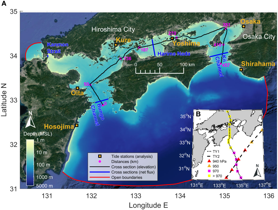
Figure 1 (A) Bathymetry of the Seto Inland Sea (SIS). The orange square marks are the locations of the tide stations used for analysis of the model results. The black line indicates the cross section for the surface elevations shown in Figure 4. The blue line cross sections are used for the net flux analysis. (B) Pathways of TY1 and TY2 (Typhoon TALAS and Typhoon ROKE, respectively). Triangular and square marks indicate central air pressures of typhoons.

The sea level distribution of the SIS has distinct characteristics. Basically, the sea level in the Bungo Channel is higher than that in the Kii Channel (west high-east low), inducing easterly throughflow in the SIS (Kurogi and Hasumi, 2019; Nakatani et al., 2020). Nakatani et al. (2020) suggested that the throughflow via the sea level gradient is related to the Kuroshio current. Kurogi and Hasumi (2019) calculated the volume transport of seawater across the SIS. They found that considering tidal effects, such as vertical diffusivity and viscosity and the generation of tidal residual eddies, was important for calculating transport precisely. Volume transport has a more significant effect on the semienclosed SIS because the mean current transporting materials are highly responsible for keeping the marine environment clean and healthy. Despite these modeling studies, the roles of detailed net flux on basin-wise sea level variations and abnormal surges in Hiroshima Bay have not yet been fully addressed.

The previous study by the authors (Jeong and Lee, 2023) focused on setting up the model system and obtaining the reliability of the model for the SIS with an application to storm surge in Osaka Bay Typhoon Jebi in 2018. On the other hand, the current study focused on the abnormal tides in Hiroshima Bay in September 2011 to investigate the coastal and ocean process of the abnormal tides and to reveal the effects of external processes on the event. The SIS model of this study is an extended and improved version of the previous Hiroshima Bay model in Jeong et al. (2023). The previous Hiroshima Bay model could not consider the effects from external processes such as river discharges, the circulations in the SIS, the Kuroshio current and effects from Pacific Ocean. However, after the extension of the computation domain, the SIS model can consider river discharges, the SIS circulation and corrected the sea surface height (SSH) of the SIS model at open boundaries, thereby successfully simulating abnormal sea level rise in Hiroshima Bay.

Thus, in this study, we adopted an unstructured mesh-based high-resolution hydrodynamic model for the SIS to elucidate the cause and process of the abnormal tide in the bay and the relationship with the sea level variation and circulation in the SIS, by analyzing the net flux in each channel and suggesting the major role of each channel in determining the sea level variation and circulation in the SIS. The patterns of sea level and circulation characteristics in the SIS are not only needed by physical oceanographers for coastal and ocean process, natural hazards, particle tracking of river-borne debris, etc., but also in biological and geochemical oceanography fields for sea grass denudation, seed spreading and nutrient distributions. In addition, there are numerous semi-enclosed seas in various scale in the world, for example the largest Mediterranean Sea, thereby the findings of this study will give insights not only to local stakeholders but also to global readers related to similar coastal and ocean environment.

In the following text, the model setup and statistical indices used in this study are described in Section 2. In Section 3, model validation and comparisons of subtidal elevation and net fluxes before and after open boundary correction are described. Section 4 presents the results of a comparison between the Hiroshima Bay-scale model and the SIS-scale model. Conclusions are provided in Section 5.

2 Materials and methods

2.1 The Seto Inland Sea model: SCHISM

The semi-implicit cross-scale hydroscience integrated system model (SCHISM by Zhang et al., 2016) was adopted in this study to simulate an abnormal tide that occurred in Hiroshima Bay and the SIS. This model is a derivative product based on the original SELFE model (v3.1dc) (Zhang and Baptista, 2008). The Navier-Stokes equations are solved in hydrostatic form using semi-implicit finite-element/volume methods, which reduce Courant-Friedrichs-Lewy (CFL) stability constraints and increase numerical efficiency. A higher-order scheme for momentum advection with Explicit Locally Adaptive Dissipation (ELAD) filter is applied to the SCHISM to control excess mass with an iterative smoother. Total Variation Diminishing with two limiter functions (TVD²) is a higher-order implicit advection transport scheme using two space and time limiters. This allows the model to conserve baroclinic instability without filtering out, successfully capturing smaller eddies. These characteristics allow seamlessly stable simulations across varying scales from the creek, lake, river, estuary, shelf to the ocean (Zhang et al., 2023). The model domain in this study included a river (approximately 3 m deep) and the Nankai Trough (approximately 4,900 m deep) with narrow straits and complicated geometry. Therefore, the SCHISM will be an appropriate numerical model for the SIS.

The fundamental equations of the SCHISM model consist of three equations: (Equation 1) the continuity equation, (Equation 2) the momentum equation, and (Equation 3) the transport equation.

$\begin{array}{ll}\nabla ·\mathit{\text{u}}+\frac{\partial w}{\partial z}=0& (1)\end{array}$

$\begin{array}{ll}\frac{D\mathit{\text{u}}}{Dt}=\frac{\partial }{\partial z}(\nu \frac{\partial u}{\partial z})-ɡ\nabla \text{η}+F& (2)\end{array}$

$\begin{array}{ll}\frac{DC}{Dt}=\frac{\partial }{\partial z}(\kappa \frac{\partial C}{\partial z})+{\text{F}}_{\text{h}}+Q& (3)\end{array}$

where $(x, y)$ are the horizontal coordinates, $z$ is the vertical coordinate, $t$ is the time, $\mathit{\text{u}}(x, y, z, t)$ is the horizontal velocity, $w$ is the vertical velocity (upward), $\text{η}(x, y, t)$ is the free surface elevation, $g$ is the gravitational acceleration, and $C$ is the concentration of the tracer, such as temperature and salinity. $\nu$ is the vertical eddy viscosity, $\kappa$ is the vertical eddy diffusivity for the tracer, and F is the additional momentum forcings such as the Coriolis effect and air pressure. ${\text{F}}_{\text{h}}$ is the horizontal diffusion, and $Q$ is the source/sink mass of the tracers.

To enhance momentum stabilization, (Equation 4) a 5-point Shapiro filter (Shapiro, 1970) was adopted in this study. There are different tools, such as the Laplacian viscosity and biharmonic viscosity, which act similarly to the Shapiro filter. However, the filter is suitable for noneddying regime applications, such as nearshore areas, estuaries, and rivers, because of the following equation:

$\begin{array}{ll}\widetilde{u_0}=u_0+\frac{\gamma }{4}(u_1+u_2+u_3+u_4+-4u_0)& (4)\end{array}$

where $u_0$ is the velocity at side ‘0’, which is defined between two elements (here, triangular), and $u_n$ (n = 1, 2, 3, and 4) is the velocity defined at the other two sides of two triangles (2×2 = 4). γ is a nondimensional Shapiro filter parameter used to define the strength of stability. It is recommended that this parameter be set between 0 and 0.5, and different values of the parameter can be assigned to each node depending on the model instability. To investigate mass exchanges through straits and similar narrow passages, when side velocities are converted to a node velocity in the Shapiro filter, the 5-point Shapiro filter is used again to redistribute excess mass. Therefore, excess mass is redistributed and conserved between sub-basins through straits.

2.2 Model setup

The unstructured mesh covering the Seto Inland Sea and adjacent seas, each with a length of 500 km × 420 km, consisted of 210,505 nodes and 390,461 cells (triangular mesh in Figure 2). The horizontal resolution of the mesh varied from approximately 30 m (near the Ota River mouth and Hiroshima city) to 9,800 m (along the open boundary) depending on the geometry of the coastlines, target areas, and gradients of bathymetry. The 30-m resolution was applied only to the areas shallower than 10 m, while other narrow straits had an approximately 100-m resolution. Considering that the average depth of the SIS is around 38 m, we aimed to avoid situations where the model mesh becomes excessively fine compared to the depths. As a result, the unstructured mesh of the SCHISM model can resolve the complicated coastline geometry of the SIS.

Figure 2

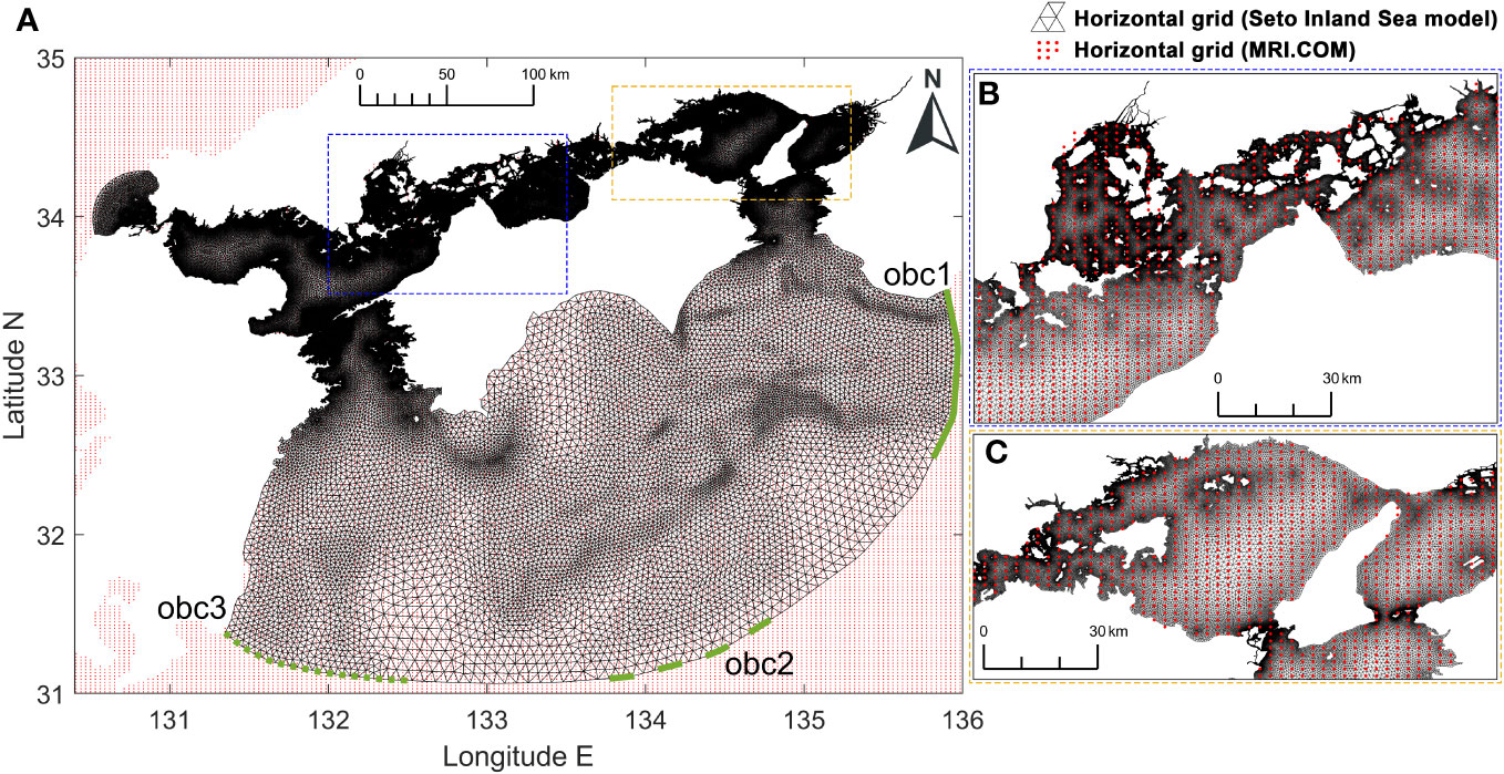
Figure 2 (A) Unstructured grid-based high-resolution mesh of the SIS model (black triangles) and structured grid-based mesh of the MRI.COM-JPN model (red dots). (B) and (C) depict both mesh around Hiroshima Bay and Osaka Bay, respectively.

The simulation period was set to 61 days from 10 August to 9 October 2011, which included an abnormal tide event in Hiroshima Bay and two typhoon events. The model was calculated with an interval of 80 seconds. The model output has a 20-minute interval. All the descriptions regarding time used in this paper are based on local time and Japan Standard Time (JST).

Spatially varying filtering parameters were applied using the 5-point Shapiro filter for the sake of numerical stability based on the maximum current velocity and horizontal resolution at each node, with higher values applied to narrow straits and river mouth areas where numerical instability can occur due to strong currents. As a result, 0.2 of the parameters for the normal areas and a maximum of 0.5 for the unstable areas were given. This approach allowed us to increase the model resolution near narrow straits with strong currents frequently developed while the model stability was maintained. The detailed descriptions of the model setup are documented in Jeong and Lee (2023).

Thirty vertical layers in σ coordinate were adopted in the SIS model and LCS² grid (Localized Sigma Coordinates with Shaved Cells) was applied in the model to reduce the instability and pressure gradient error at areas with narrow straits and shallow or steep depths. In addition, the current σ-layer adopted in this study didn’t show significant errors during the simulation, as validated well with field measurements (Jeong and Lee, 2023).

The bottom roughness length ($z_0$) used near the bottom boundary layer was applied nonuniformly in this study. A higher value of the parameter was defined as the depth ($D$) increase (Equation 5), following the approach of Cowles et al. (2008).

$\begin{array}{ll}{z}_0\{\begin{array}{cc}\begin{array}{l}3\times {10}^{-3}\\ 3\times {10}^{-3}{\exp }^{-(D-40)/8.8204}\\ 1\times {10}^{-4}{\exp }^{-(D-70)/13.0288}\\ 1\times {10}^{-5}\end{array}& \begin{array}{l}ifD\le 40\\ if40<D\le 70\\ if70<D\le 100\\ if100<D\end{array}\end{array}& (5)\end{array}$

2.3 Forcing data

SIS modeling considers external forcings, such as tides, sea surface height (SSH), water temperature, currents, surface winds, air pressure, and river discharge, which can affect sea level changes directly or indirectly. Table 1 describes all the datasets used in the model. The Japanese Meteorological Agency (JMA) Meso-Scale Model (MSM) offers high-resolution data (approximately 5 km) near Japan. Therefore, the MSM was adopted for the hourly surface winds, air pressure, and air temperature, while ERA5 was utilized for hourly precipitation and radiation dew point temperature after interpolation to a grid of the MSM. The specific humidity was calculated from the dew point temperature and air pressure fields of ERA5. Detailed descriptions regarding how each dataset was treated are documented in Jeong and Lee (2023).

Table 1

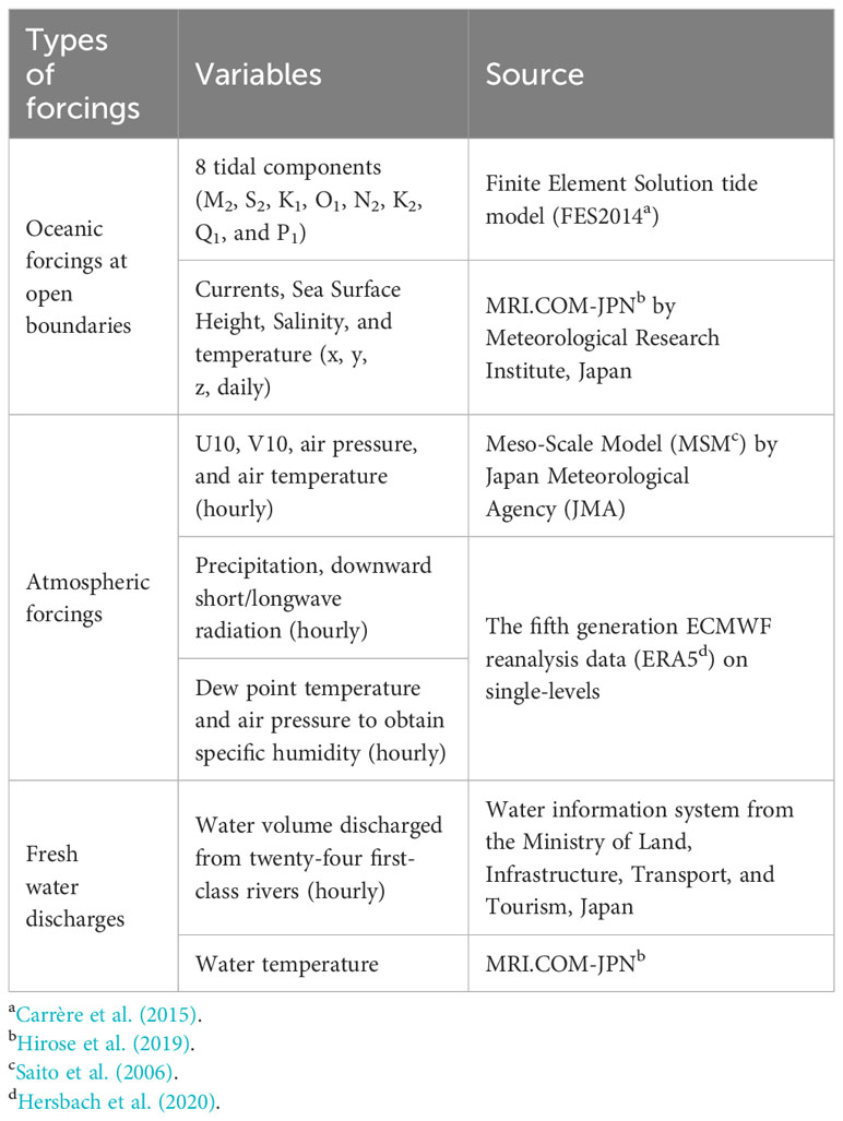
Table 1 Variables and their sources used in the hydrodynamic model of the Seto Inland Sea as forcings.

The MRI.COM-JPN model from the JMA was utilized primarily for the initial field and boundary forcings in the ocean component of our study. Notably, the model employs a structured grid with an approximate resolution of 2 kilometers, as illustrated in Figure 2. This MRI.COM-JPN was developed by the JMA to enhance coastal monitoring and forecasting systems, covering a wide area from the SIS to the entire coastal seas of Japan (Sakamoto et al. (2019). In contrast, the SIS model, implemented using SCHISM, focuses on the SIS and its immediate vicinity, providing much higher resolution, as demonstrated in Figure 2.

2.4 Evaluation of the model results

The mean absolute error (MAE) and index of agreement (IOA) (Willmott et al., 2012) were calculated to evaluate the model results. The MAE is a dimensioned measure of average model performance error expressed in units of the variable of interest (Willmott, 2005). The MAE is described as in Equation 6:

$\begin{array}{ll}MAE=\frac{{\sum }_{i=1}^n\left|P_i - O_i\right|}{n}& (6)\end{array}$

where $P_i$ is the i_th model result, $O_i$ is the i_th observation, and n is the number of data points.

The IOA adopted in this study is a refined version of the original Willmott’s dimensionless IOA (Willmott, 1981). The refined IOA has a lower limit of −1 and an upper limit of +1, which is double the range of the original IOA (from 0 to +1). The refined IOA is calculated via Equation 7:

$\begin{array}{ll}\text{IOA\hspace{0.17em}}=\{\begin{array}{l}1-\frac{1}{2}\frac{{\displaystyle {\sum }_{i=1}^n|P_i-O_i|}}{{\displaystyle {\sum }_{i=1}^n|O_i-\overline{O}|}},when{\displaystyle {\sum }_{i=1}^n|P_i-O_i|\le 2{\displaystyle {\sum }_{i=1}^n|O_i-\overline{O}|}}\\ \frac{2{\displaystyle {\sum }_{i=1}^n|O_i-\overline{O}|}}{{\displaystyle {\sum }_{i=1}^n|P_i-O_i|}}-1,when{\displaystyle {\sum }_{i=1}^n|P_i-O_i|>2{\displaystyle {\sum }_{i=1}^n|O_i-\overline{O}|}}\end{array}& (7)\end{array}$

The upper equation in Equation 7 is used when the IOA is positive. Basically, an IOA value closer to +1 indicates better performance of a numerical model. When IOA = +0.5, the sum of the absolute errors is half of the sum of the deviation magnitudes of the perfect model and observation. When IOA = 0, Equation 7 is equivalent. If the IOA becomes negative (−0.5, for example), the sum of the absolute errors is double the sum of the deviation magnitude of the perfect model and observation.

2.5 Calculation of net flux budget

The SCHISM model utilizes an unstructured triangular mesh system, making it challenging to depict a straight line for cross-sectional analysis. Therefore, model results were interpolated at new grid points, located along the cross section, as illustrated in Figure 3A. Net fluxes (m³/s) were then calculated by multiplying the velocity normal to the cross section (m/s) and the area (m²) at each grid point, as described in Equation 8. The area at each grid point was obtained by calculating the area of the trapezoid, as depicted in Figure 3B, and expressed in Equation 9. The cross-sectional net flux at a specific time was obtained by summing net fluxes calculated at all mesh and at all vertical layers, as presented in Equation 8.

Figure 3

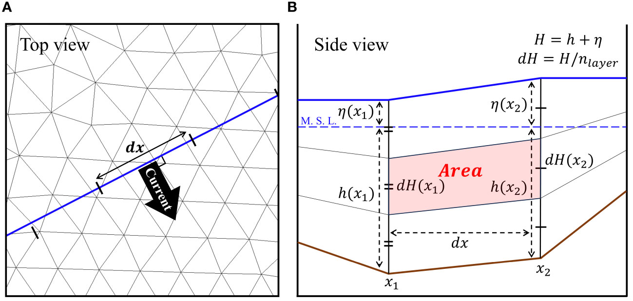
Figure 3 Schematic method to calculate net flux budget. (A) Top view for the cross section and normal velocity. (B) Side view for the calculation of the area.

$\begin{array}{ll}Netflux(t)={\displaystyle {\sum }_{x=1}^{N-1}{\displaystyle {\sum }_{\text{z}=1}^{30}\left(Area(x,z,t)\times U_n(x,z,t)\right)}}& (8)\end{array}$

$\begin{array}{ll}Area(x,z,t)=\frac{1}{2}\left(dH(x,z,t)+dH(x+1,z,t)\right)\times dx& (9)\end{array}$

Here, $N$ is the number of grid points at each cross section, $z$ is a vertical layer (maximum 30^th layer), $U_n$ is the velocity normal to the cross section, and $H$ is the total depth.

The number of grid points was determined based on the length of each cross section to achieve consistent resolutions for net flux calculations. For instance, in the Bungo Channel (See Table 2), the length of the cross-sectional line is 29.12 km. It was divided into 101 grid points, making a final resolution of approximately 300 m. Similarly, for other channels, the number of grid points was determined in proportion to their respective lengths, resulting in a cross-sectional resolution of approximately 300 m.

Table 2

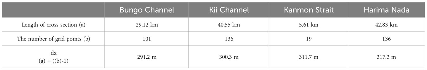
Table 2 Cross-sectional analysis information in the Seto Inland Sea.

3 Results

Figure 4 shows the west-east patterns of sea surface elevations extracted from the corrected model results along a cross section in the SIS, as indicated by the solid black line in Figure 1. The correction process is described in Section 3.3. This result also depicted a spatial distribution of sea level similar to that described in the literature (Kurogi and Hasumi, 2019; Nakatani et al., 2020). The 61-day-averaged surface elevation (black solid line in Figure 4) exhibited an analogous west-high-east-low pattern, a basic structure in the spatial distribution of sea surface elevation. However, the spatial pattern changes depending on meteorological or oceanic events, such as typhoons and abnormal tides, as detailed in Section 3.4.

Figure 4

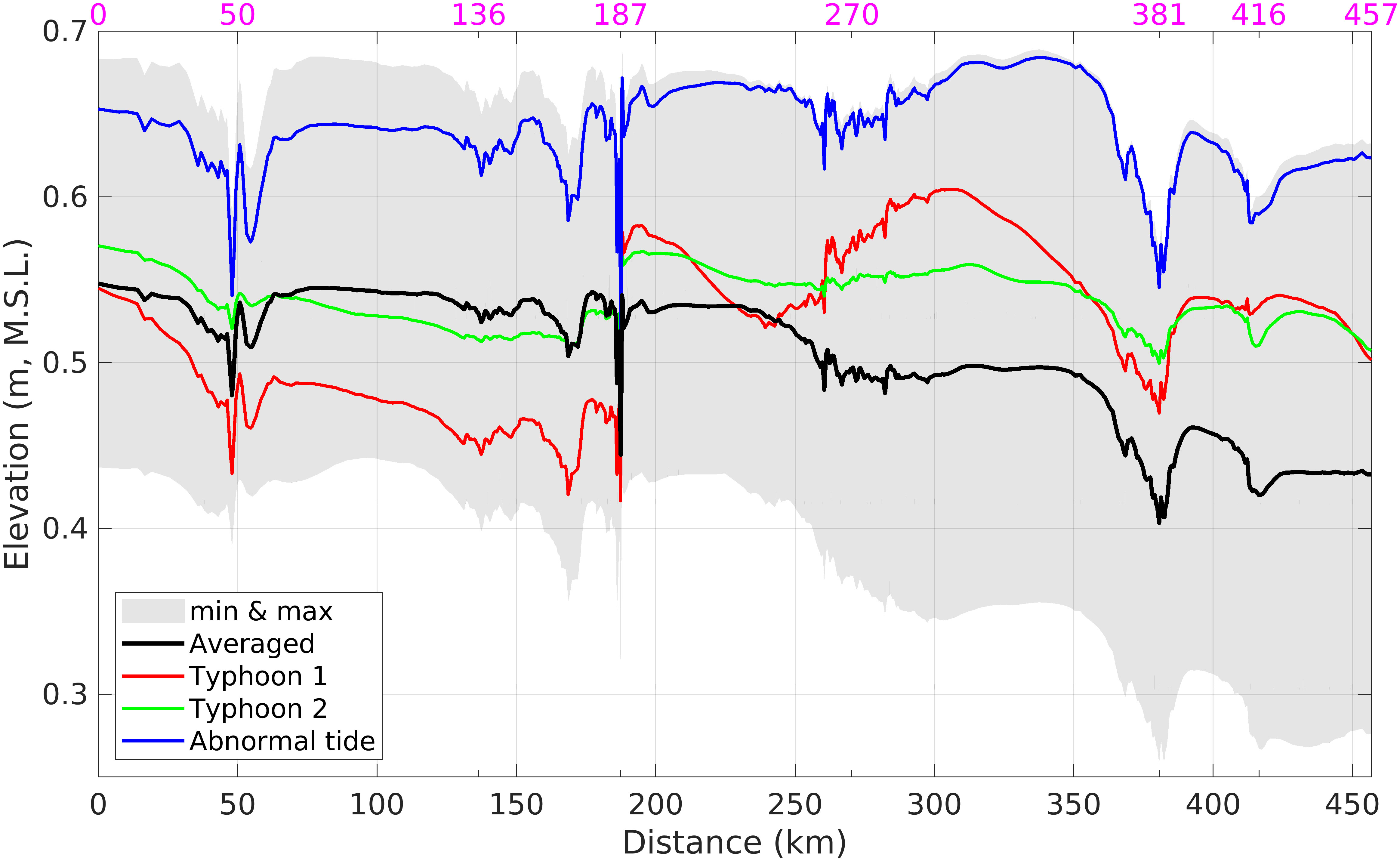
Figure 4 2-day-averaged surface elevations extracted from the model results along the west-east cross section in Figure 1. The red and green lines indicate the sea level variation patterns when typhoons (TY1 and TY2) passed or approached the SIS, respectively. The blue line represents the west-east sea level variation when an abnormal tide occurred in Hiroshima Bay. The black line indicates the 60-day-averaged surface elevation, with the gray shading indicating the range of sea level variation for 60 days.

The model results regarding surface elevation, temperature, and currents have been validated with measurement data from fifty-six observation stations [Jeong and Lee (2023)]. In Jeong and Lee (2023), the amplitudes (phases) of tidal constants were approximately 0.04 (0.01) of the normalized root-mean-square error (NRMSE) when comparing the model results with observations from forty-two tide stations. The velocity profile from the bottom to the surface layers exhibited reasonable results compared to those of mooring observations, with NRMSE values ranging from 0.11 to 0.17. Seasonal and weekly fluctuations in water temperature were well reproduced at thirteen stations. For additional detailed validation results, please refer to Jeong and Lee (2023) for the sake of brevity.

For further analysis of sea level variation, among the forty-two tide stations, we selected six stations—Kure, Oita, Osaka, Yoshima, Hosojima, and Shirahama—as shown in Figure 1. These stations are distributed throughout the model domain from the main open boundary to the innermost SIS. In this section, we analyzed the model results at these stations. In particular, the Kure tide station is located near Hiroshima city and the Ota River, where the Itsukushima Shrine is present. The Hiroshima tide station is located closest to the shrine; however, Hiroshima station data were not considered in the analysis due to missing data during the research period.

3.1 Tides

The magnitude of the tides changed as they propagated inside the SIS. The maximum tidal range at Kure station (Figure 5B) was approximately 3.9 m with semidiurnal characteristics (Jeong and Lee, 2023), whereas Hosojima (Shirahama) station in the outer SIS presented low amplitudes of approximately 2 m (1.9 m), as shown in Figures 5D, E. However, Osaka station, located in the eastern part of the SIS, had a lower amplitude of 1.5 m, and diurnal tides became dominant during neap tide. This spatial distribution of tides from the observation and the model matched Yanagi et al. (1982).

Figure 5

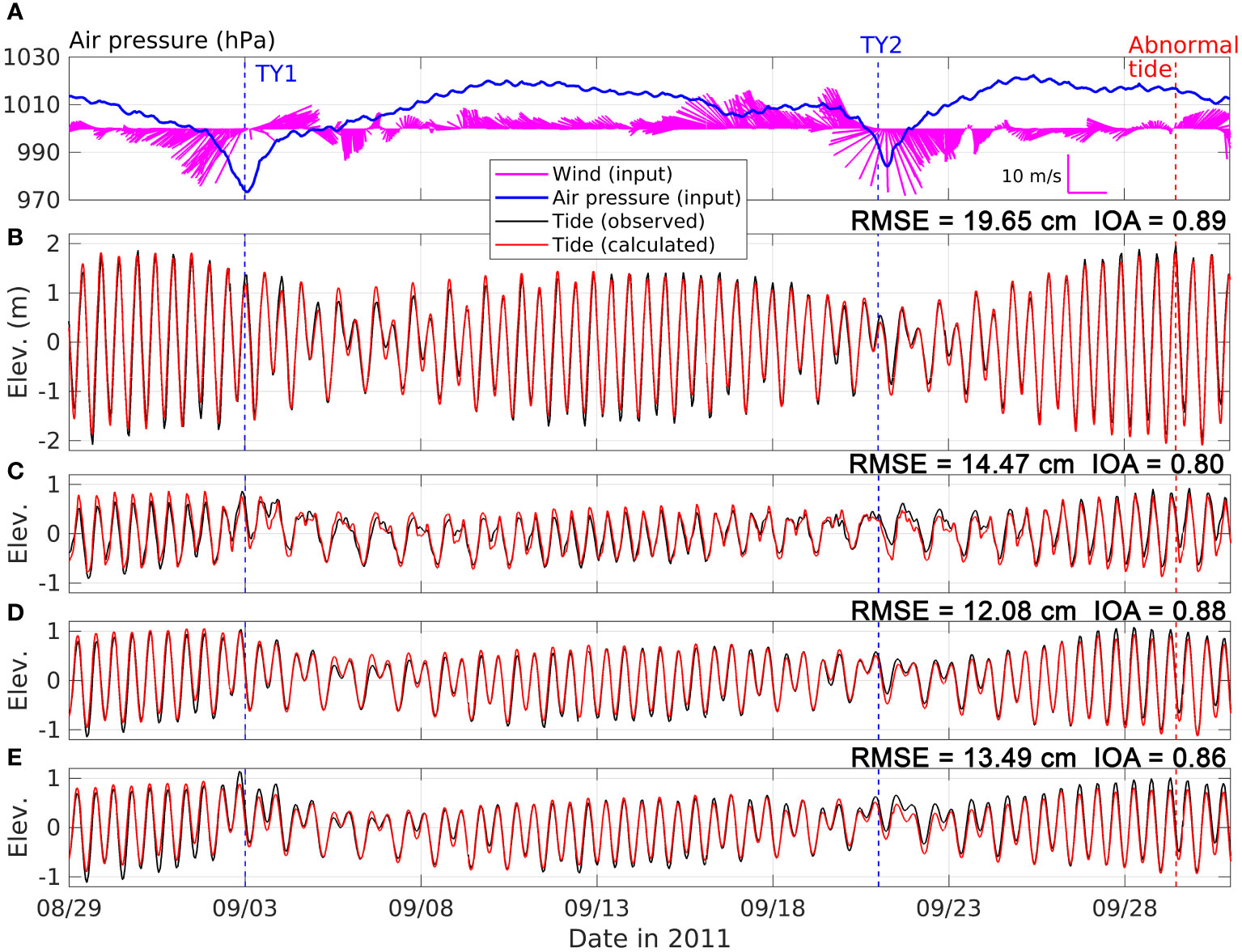
Figure 5 Surface elevations at the (B) Kure, (C) Osaka, (D) Hosojima, and (E) Shirahama stations. The black (red) lines indicate the observations (SIS model results). (A) Air pressure and wind vectors from JMA MSM model at the center of the model domain (33.237° N, 133.652° E) indicating the representative conditions in the SIS.

Elevation data from tide stations can capture not only tidal signals but also other subtidal components. The subtidal is used to express the signals which are obtained after excluding dominant tidal signals (Payandeh et al., 2019; Laurel-Castillo and Valle-Levinson, 2020) such as storm surges, abnormal tides, and non-tidal long waves. It does not necessarily be shorter than semi-diurnal tide in this study. The long waves mainly indicate CTWs such as edge waves, Kelvin waves, and continental shelf waves including the planetary edge waves. Figure 5A shows the wind vectors (magenta) and air pressure (blue) from the JMA MSM model at the center of the model domain (133.65° E, 33.24° N), indicating the representative condition in the SIS. Two typhoons, TY1 and TY2, passed through the SIS during the simulation period. As TY1 approaches the SIS, low air pressure (973 hPa) and strong winds disturb seawater, causing sea level variations, as shown in Figures 5C, E. However, because tidal components are more dominant than these variations are, it is difficult to distinguish subtidal components from tides.

3.2 Subtidal elevation

Daily averaged elevations were calculated to investigate subtidal variations, as shown in Figure 6. The observed subtidal elevations at all stations in Figure 6 exhibit a peak when an abnormal tide occurred. This indicates that abnormal tides occurred not only in Hiroshima Bay but also throughout the whole SIS, and they can be observed at the outer stations of the SIS. Furthermore, at the Osaka, Yoshima, and Shirahama stations, located in the relatively eastern part of the SIS, one more peak was observed due to the storm surge when Typhoon 1 approached the SIS.

Figure 6

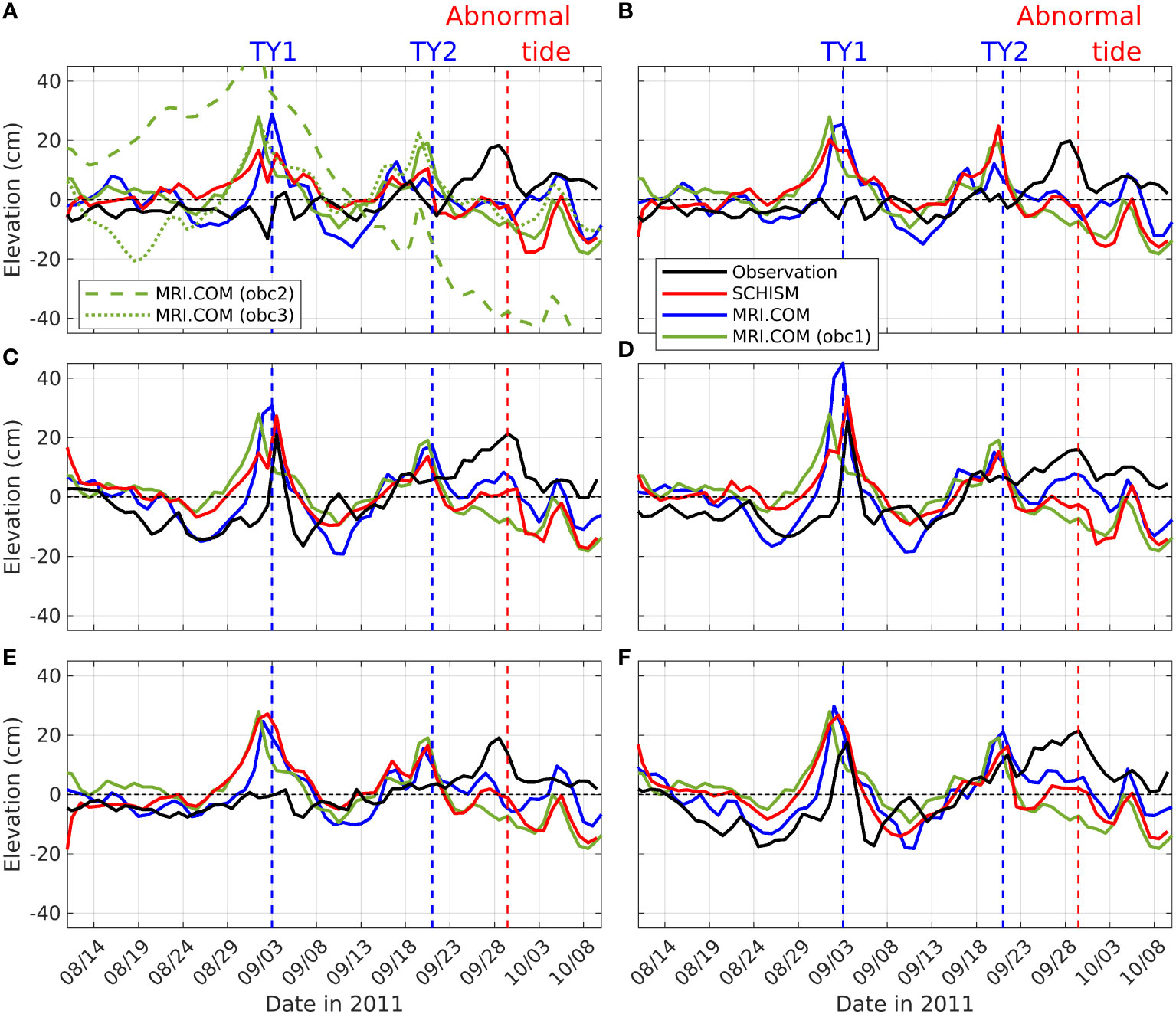
Figure 6 Daily averaged elevation at the (A) Kure, (B) Oita, (C) Osaka, (D) Yoshima, (E) Hosojima, and (F) Shirahama stations. The black (red) lines indicate the observations (SIS model results). The blue (green) lines indicate the elevations extracted from MRI. COM-JPN data at tidal stations (open boundaries). The locations of obc1 to obc3 are presented in Figure 2A. The dotted vertical lines indicate the timings of Typhoons 1 and 2 and the abnormal tide.

For comparison, to remove the influence of tides in the subtidal data analysis, the T-Tide and T-Predic software were applied and the result at Kure station is shown in Figure A1. The daily-averaging method and the T-Tide application results did not show significant difference in subtidal components.

The results from the SIS model could not reproduce these peaks at TY1 and abnormal tide. To investigate why the model failed to describe this phenomenon, sea surface height (SSH) from MRI.COM-JPN utilized as initial and open boundary conditions was compared with the observed and SIS model results in this study. In the comparison, we noticed that MRI.COM-JPN (blue lines in Figure 6) could not reproduce subtidal components well. The difference in SSH in MRI.COM still remained at the location of the open boundary of the SIS model (green lines in Figure 6). Therefore, additional simulations were conducted after correcting the SSH bias at the open boundary. Moreover, interestingly, the subtidal elevation at obc1 had the highest correlation coefficient (r = 0.77) with the SIS model results, although obc2 (r = 0.70) and obc3 (r = 0.57) were closer to the Kure, Oita, and Hosojima stations. This difference might be related to CTWs, as stated by Usui et al. (2021).

3.3 Sea surface height at the open boundary

To improve the SIS model results and reduce the SSH open boundary conditions, elevations defined at the open boundary were corrected using differences between the observations and the results of the SIS model (ad hoc correction). The Hosojima and Shirahama tidal stations, which are the closest stations to the western and eastern sides of the open boundary, respectively, were chosen for bias correction. As tidal waves propagate further, the waves can be transformed and amplified in the SIS. Therefore, the stations closest to the boundary were adopted to correct the SSH at the boundary.

Figure 7 shows the water level differences between the observation and model results at the Hosojima and Shirahama tidal stations, and these differences are identical to the corrected water levels at the boundary. When correcting the boundary conditions, spatially varying modifications depending on the distance from two stations are considered. In detail, there were 106 nodes at the open boundary, and for the most western (eastern) nodes, we added the difference in subtidal elevation calculated at the Hosojima (Shirahama) station. Then, we interpolated the differences for the other open boundary nodes according to the distances to both ends (the most western and eastern nodes). The ten green lines in Figure 7 represent samples of the interpolated gaps at ten open boundary nodes among the 106 nodes.

Figure 7

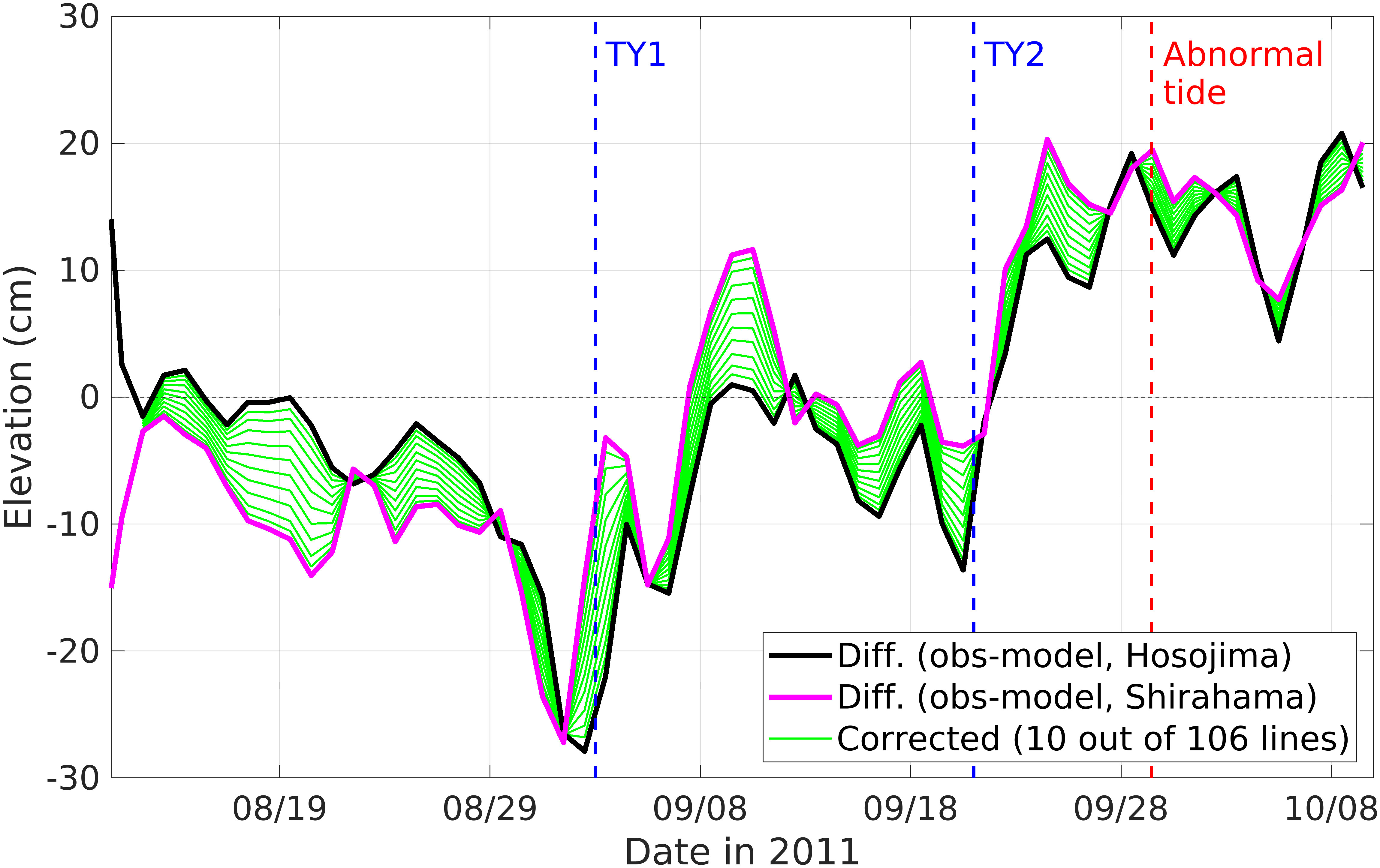
Figure 7 Differences in subtidal elevation calculated at Hosojima and Shirahama stations. The green lines indicate the differences interpolated at ten nodes among the 106 open boundary nodes.

Another simulation (blue solid lines in Figure 8) used the same model configuration as the previous simulation and was conducted after the correction was applied. The correction process effectively improved the model results, achieving a lower MAE and higher IOA, as shown in Table 3. The MAEs at subtidal elevations at all stations were markedly reduced. Before correction, the average MAE at the six stations was approximately 9.19 cm. However, after the correction, the value decreased to 3.15 cm, representing a reduction of 66%. Especially at the Osaka and Shirahama stations, the MAE was reduced by approximately 7.45 cm, which accounts for 77% of the original MAE at these stations. These stations were located on the eastern side of the model domain, close to the eastern open boundary, where we utilized the subtidal component for the correction.

Figure 8

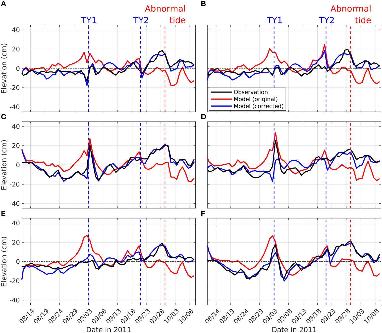
Figure 8 Subtidal elevations from three datasets: observations (black), model results before correction (red), and model results after correction (blue). (A) to (F) indicate the same tide stations as in Figure 6. The dotted vertical lines indicate the timing of Typhoons 1 and 2 and the duration of the abnormal tide.

Table 3

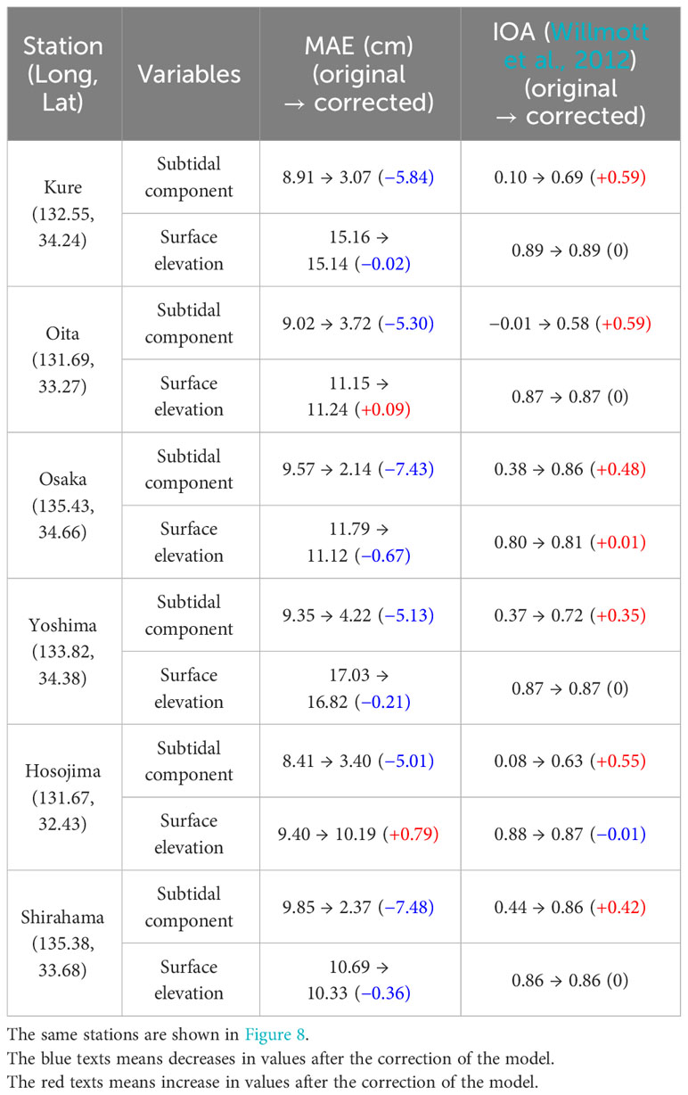
Table 3 Mean absolute error (MAE) and index of agreement (IOA) before and after the SSH correction at the open boundary.

The IOA increased by 0.55 (from 0.08 to 0.63) at Hosojima station, closest to the western side of the open boundary, and increased by 0.42 (from 0.44 to 0.86) at the Shirahama station, closest to the eastern side, after the boundary correction. As the subtidal elevation propagated into the SIS, the average IOA in the SIS also improved by 0.50 (from 0.21 to 0.71). In particular, significant improvements were observed at the Kure station, which is located close to the Itsukushima Shrine, where flooding occurred. After correction, the IOA at this station reached 0.69. Regarding the surface elevation before extracting the subtidal component, the IOA did not change significantly because tides were dominant compared to the subtidal component (see the difference in the scales between Figures 5, 6). With respect to the interpretation of the IOA values, it has only statistical meanings for goodness-of-fit of the model result rather than providing threshold values for acceptable model performance in this study. Thus, the interpretation of the IOA values rests with the readers’ judgment.

From an eventwise perspective, the correction effectively improved the calculation of abnormal tides compared to that in the original case at all stations. For Typhoon 1, the nonexistent peak that was previously calculated at the Kure, Oita, and Hosojima stations (red solid lines in Figures 8A, B, E, respectively) was corrected and disappeared after the SSH correction was applied. This erroneous peak originated from MRI.COM-JPN data is shown in Figure 6. Conversely, at the Osaka, Yoshima, and Shirahama stations on the relatively eastern side of the SIS, a peak was observed during Typhoon 1, which was overestimated in the original case (and was also overestimated in the MRI.COM-JPN data). However, after the correction, the overestimation decreased, and the model results aligned better with the observations at the Osaka and Shirahama stations. Unfortunately, at Yoshima station, located at the center of the SIS, the model presented a lower peak than both the observation and the original model (Figure 8D). The corrected sea level at the open boundary was lower than that in other periods, especially at Shirahama station (smaller than 3.9 cm, magenta line in Figure 7) during the period of Typhoon 2. However, an elevation of approximately -13.6 cm was corrected at the most western node during Typhoon 2 (black line in Figure 7). Despite these corrections, only 6.4 cm decreased at the Oita and Hosojima stations close to the western node, which is less than half of the corrected elevation.

3.4 Net flux budget of the Seto Inland Sea

Net seawater fluxes crossing the Bungo Channel, Kii Channel, Kanmon Strait, and Harima Nada (Figure 9) were analyzed to investigate the water sources that induced sea level variations and changes in the sources after correction. The net fluxes were averaged daily to remove tidal signals. The locations of the cross sections are presented in Figure 1. Since the SIS is a semienclosed sea with only three passages, the Bungo Channel, the Kii Channel, and the Kanmon Strait, it is possible to calculate the net influx of seawater into the SIS (black lines in Figure 9). We also took discharged fresh water from 23 out of 24 rivers into account in the net flux budget calculation. One river located outside the cross section (not shown here) was not considered in the calculation. The solid (dotted) lines represent the net fluxes from the corrected (original) case. Positive (negative) values indicate inflow into the SIS (outflow from the SIS), respectively. Positive (negative) values at Harima Nada indicate eastward (westward) flow in the SIS.

Figure 9

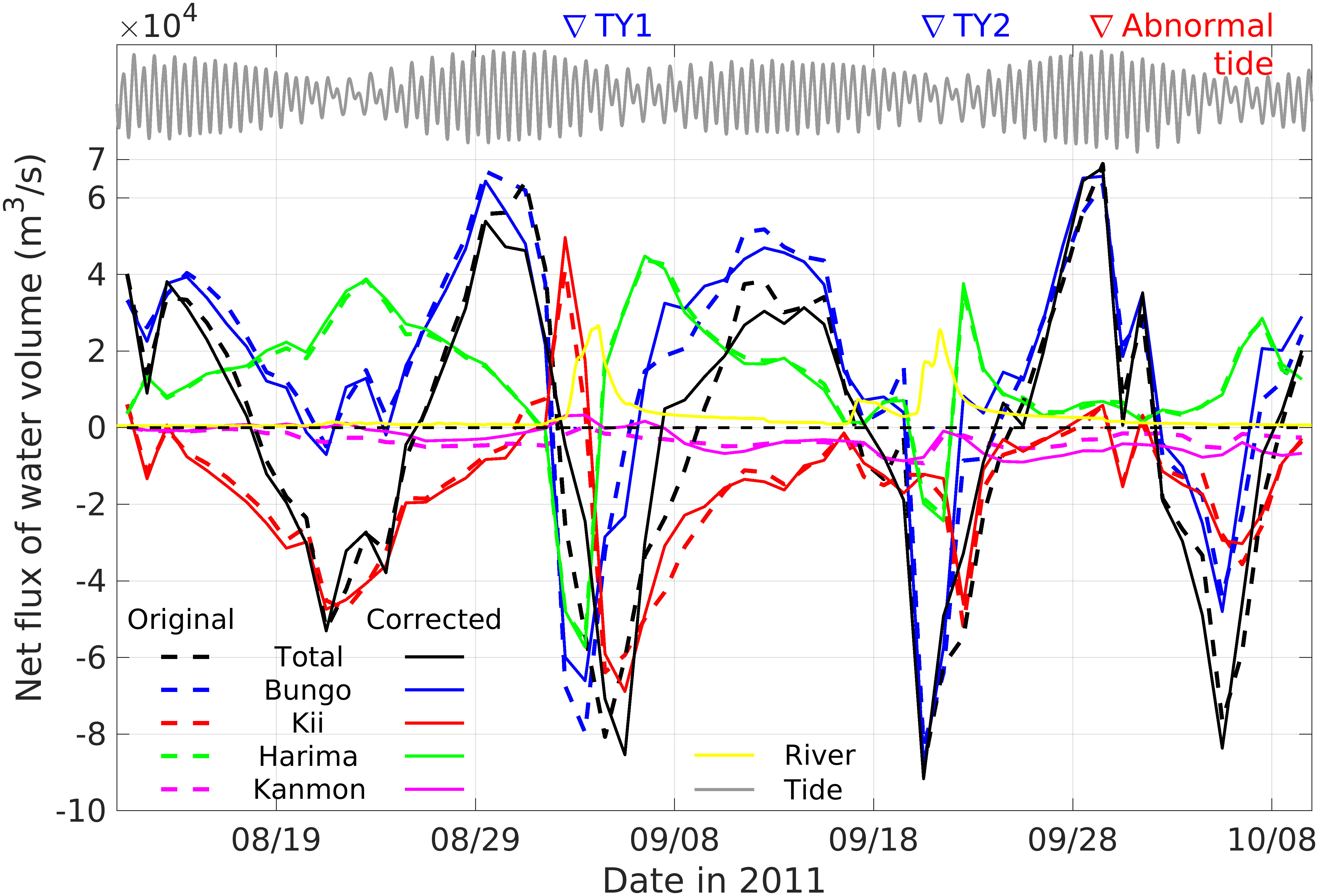
Figure 9 Daily averaged net fluxes of seawater crossing the Bungo Channel (blue), the Kii Channel (red), the Harima Nada (green), and the Kanmon Strait (magenta). The locations of these cross-sections are indicated in Figure 1. The total net flux (black) was calculated by summing the net fluxes at the Bungo Channel, the Kii Channel, and the Kanmon Strait and river discharge (yellow). Dotted (solid) lines were extracted from the original (corrected) model results. The gray line indicates the tidal elevation at the Kure tide station.

There were some similarities among the net fluxes at the cross sections in Figure 9. First, the most noticeable pattern of the total fluctuation was that of spring/neap tides. The outflow (negative) of the total was calculated for every neap tide, and it became positive as the tidal range increased. The fortnightly pattern was mainly affected by the net flux in the Bungo Channel (blue lines in Figure 9). During the second and third neap tides among the four neap tides within the simulation period, the net flux at Bungo presented sharp drops, resulting in a strong and long outflow of the net value. Except for the TY1 period, the net flux in the Kii Channel was almost negative. This means that if there is no extreme event, seawater will always be discharged along the Kii Channel, and the main inflow of seawater into the SIS will be determined by the amount of inflow at the Bungo.

Although the inflow into the SIS was mainly determined by the net flux in the Bungo Channel, water circulation could not be effectively induced at the center of the SIS (Harima Nada). The net flux at Harima Nada (green lines) did not follow the trend of the main inflow (blue lines) but rather the reverse trend of the main outflow (red lines), as depicted in Figure 9. This means that the seawater at the center flowed eastward when the seawater discharged from the Kii Channel. In other words, although there was an inflow of seawater to the Bungo Channel, the SIS would not flow eastward without discharge through the Kii Channel. As a result, inflow through the Bungo Channel tends to increase the sea level around the western side of the SIS because the inflowed sea water is not easily transferred to the eastern side without outflow through the Kii Channel.

Two countercurrents (westward) were calculated at Harima Nada during both the TY1 and TY2 events, which can be explained by the wind direction (Figure 5A) and elevation distribution across the SIS (Figure 4). The average elevation along a cross-section (black line in Figure 1) gradually decreased as it extended to the Kii Channel. This dominant gradient induced a continuous eastward net flux at Harima Nada. However, when the westward wind occurred due to typhoons (Figure 5A), spatially different patterns were calculated, and the sharp reverse gradients, which are opposite to the direction of the average gradient, appeared at a distance of 187 km (red line and green line in Figure 4). Additionally, at a distance of 270 km, a similar reverse gradient was calculated for Typhoon 1. Both locations (187 km and 270 km distances) are entrances to the Harima Nada Strait, which has very limited widths. Because of the narrow straits, each basin suffered from a storm surge. Therefore, the sea level increased near all the eastern sides of the straits (187+α and 270+α), and the sea level decreased near all the western sides of the straits (187-α and 270-α) due to the effect of the storm surge. This process induced temporary strong countercurrents at Harima Nada. However, this unstable gradient of sea level could be maintained only by the effects of the typhoons during the study period. Just after the typhoons diminished, the restoring force to recover the original gradient of the averaged elevation became dominant. The force induced strong eastward net fluxes at Hariman Nada just after the passages of TY1 and TY2, as calculated at Nada (green lines) in Figure 9.

Two additional factors contribute to the total net flux: the Kanmon Strait and river discharge. The net flux through the Kanmon Strait (magenta lines in Figure 9) was mainly outward. The reason for the constant outflow can be found in the inflow at the Bungo Channel. Because the influx in the Bungo Channel mainly induced a sea level rise around the western side of the SIS, in the Kanmon Strait, which is located on the western side, a negative outward flux is dominant for balancing the net flux. Regarding river discharge (yellow line in Figure 9), two river discharge peaks were calculated according to the timing of the typhoon: a maximum of 26,660 m³/s during TY1 and 25,557 m³/s during TY2. The river discharges were comparable to the net flux through the Kanmon Strait, implying that many rivers along the coastlines of the SIS can affect sea level variations at a limited scale in the SIS to a certain extent.

MAEs between the original model results and the corrected results for each net flux were calculated to quantify how much each net flux changed after the correction (Table 4). The largest change in the net flux after the correction was calculated at the Bungo Channel, with an MAE of 5742.2 m³/s. A strong and positive effect of the correction on the net flux in the channel can be found during TY1 and TY2. On 1 September, before TY1 approached, the corrected model calculated less inflow than the original model in the Bungo Channel. After three days, less outflow was calculated in the corrected model. These weakened flows at the Bungo Channel mitigated a nonexistent peak at the Kure and Oita stations (as described in Figures 8A, B), resulting in a smaller MAE and higher IOA of subtidal components, as shown in Table 3. For TY2, there was an insignificant difference between the original and corrected values on 21 September when TY2 approached. However, from 22 September to 30 September, the net flux of the corrected results exceeded that of the original one, indicating a greater inflow of the corrected model through the Bungo Channel. This additional inflow helped address the abnormal tide, as shown in Figure 8.

Table 4

Table 4 Mean absolute error (MAE) of the net fluxes of the original model results relative to the corrected model results at each cross section.

Other net fluxes, such as those in Kii, Kanmon, and Harima, presented slighter changes than those in the Bungo Channel, as shown in Table 4. However, these changes also helped improve the model results. For the Kii Channel, close to Osaka Station, a greater outflow was calculated from 25 August to 2 September, resulting in a slow increase in subtidal elevation at Osaka Station (Figure 8C). The reason why the subtidal component increased even under the outflow at the Kii Channel was because of an inflow from Harima Nada. The amount of inflow from Harima Nada to Osaka Bay exceeded the amount of outflow from Osaka Bay to the outside of the SIS (compare the green lines and red lines in Figure 9). Then, from 3 September to 5 September, the larger inflow and less outflow at the Kii Channel were calculated after the correction. This change induced a steep rise in sea level at Osaka station, as depicted in Figure 8C. From 21 September to 30 September, after the TY2 passed, less outflow was calculated from the Kii Channel after correction. This change caused the sea level to increase at the Osaka station (Figure 8C). Although there were modifications in the net fluxes at the Bungo and Kii Channels, the net flux at the Harima Nada did not significantly change (green lines in Figure 9).

Discharge from the Kanmon Strait acted as a buffer against sea level rises. While the net flux in the Kanmon Strait presented negative values (outflow) almost always, some differences were calculated after the correction. During the TY1 season, a relatively stronger outflow was calculated in the original season. This was because the sea level on the western side of the SIS was greater in the original model than in the corrected model at that time (Figures 8A, B). If there was no discharge from the Kanmon Strait, the sea level in the SIS would have increased.

Similarly, the opposite situation occurred during TY2. A large discharge was calculated in the corrected model, resulting from higher sea levels in the corrected model. This means that although the width of the Kanmon Strait is much narrower than that of other channels, it also plays an important role in mitigating rapid sea level rises by discharging seawater depending on sea level.

In this section, how each channel (Bungo, Kii, and Kanmon) affects sea surface heights and circulations in the SIS was analyzed. Figure 10 illustrates the spatial ranges influenced by Bungo Channel and Kii Channel. Regarding sea surface heights, nearly the entire SIS was affected by the Bungo Channel (indicated by blue and purple areas). However, the Kii Channel had a significant effect only in proximity to the channel (purple and red areas). Circulations exhibited a slightly different pattern with currents at the center of the SIS (Harima Nada) being more influenced by the currents at the Kii Channel. Sea water was usually discharged from the SIS to outside through the Kanmon Strait.

Figure 10

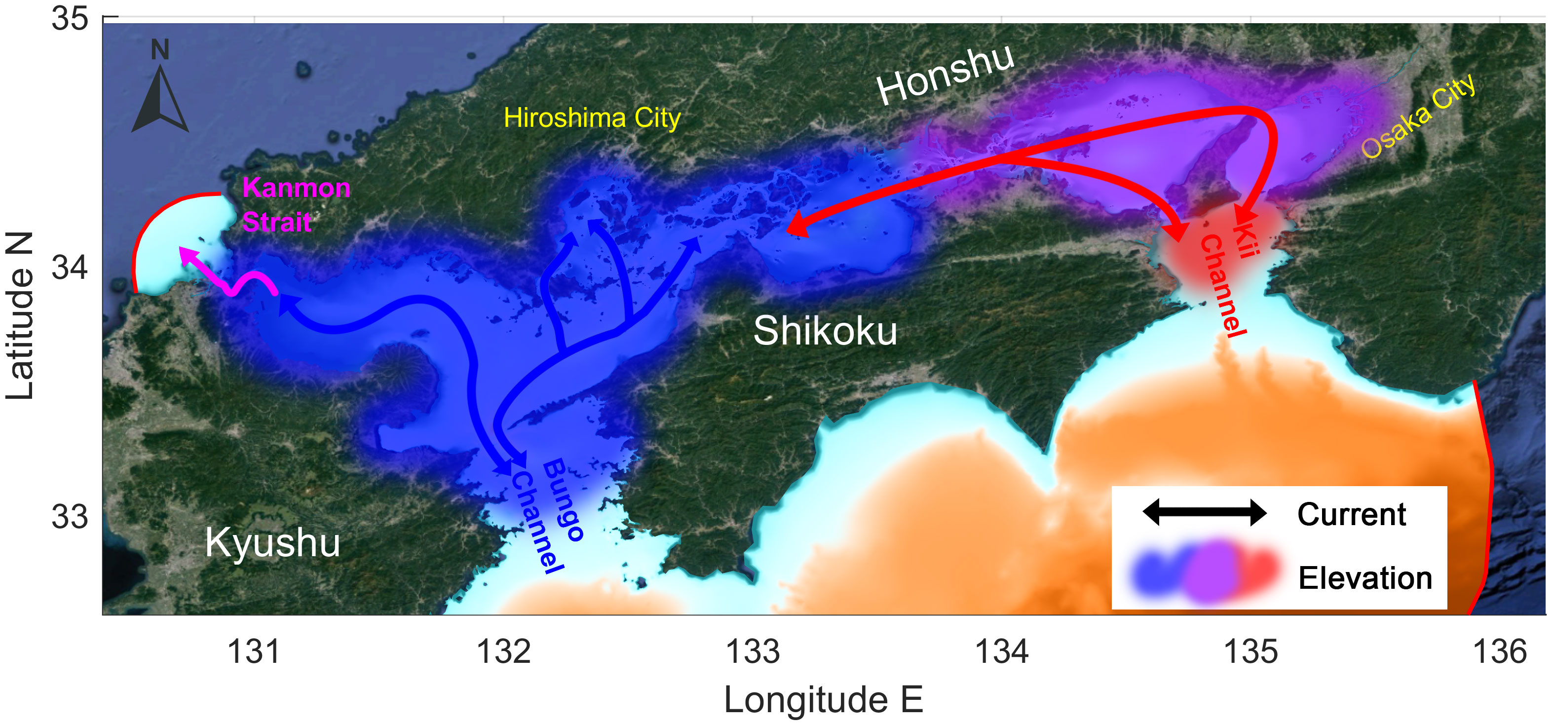
Figure 10 A schematic diagram illustrating the influence areas by each channel. Blue (red) shades indicate the area where sea surface heights are mainly determined by seawater from Bungo (Kii) Channel. Purple shades means the area where both Bungo Channel and Kii Channel give effects on the elevations.

4 Discussion

This paper corrected the original SIS model results by modifying the SSH at the open boundary using subtidal elevation differences between the observations and the model results. Previously, Jeong et al. (2023) utilized the SCHISM model to reproduce abnormal tides at the scale of Hiroshima Bay. However, the model in the earlier study covered only the bay with a domain size of 50 km × 70 km in order to analyze causal factors (internal surge) contributing to abnormal tide generation within the bay. In contrast, the current model encompasses a larger area of 500 km × 420 km. Approximately, 15% of the abnormal tide amplitude was explained by the internal surge in the previous study with uncertainties remained, particularly in terms of the phase of the abnormal tide occurrence (magenta line in Figure 11). The results of the present study significantly improved upon those of previous studies by expanding the study area, implementing boundary corrections and revealing the effects of each channel, basin and the circulation of the SIS. Nevertheless, some disparities between the observations and the SIS model persisted. The SIS model calculated an 8.5 cm-higher elevation than the observation at approximately 11 September, as depicted in Figure 11. Additionally, the model reproduced a subtidal component of only 15 cm during the abnormal tide, whereas the observed height was approximately 18 cm. A 3 cm difference was primarily observed in the western part of the SIS, with more accurate calculations of the abnormal tide occurring in the eastern part.

Figure 11

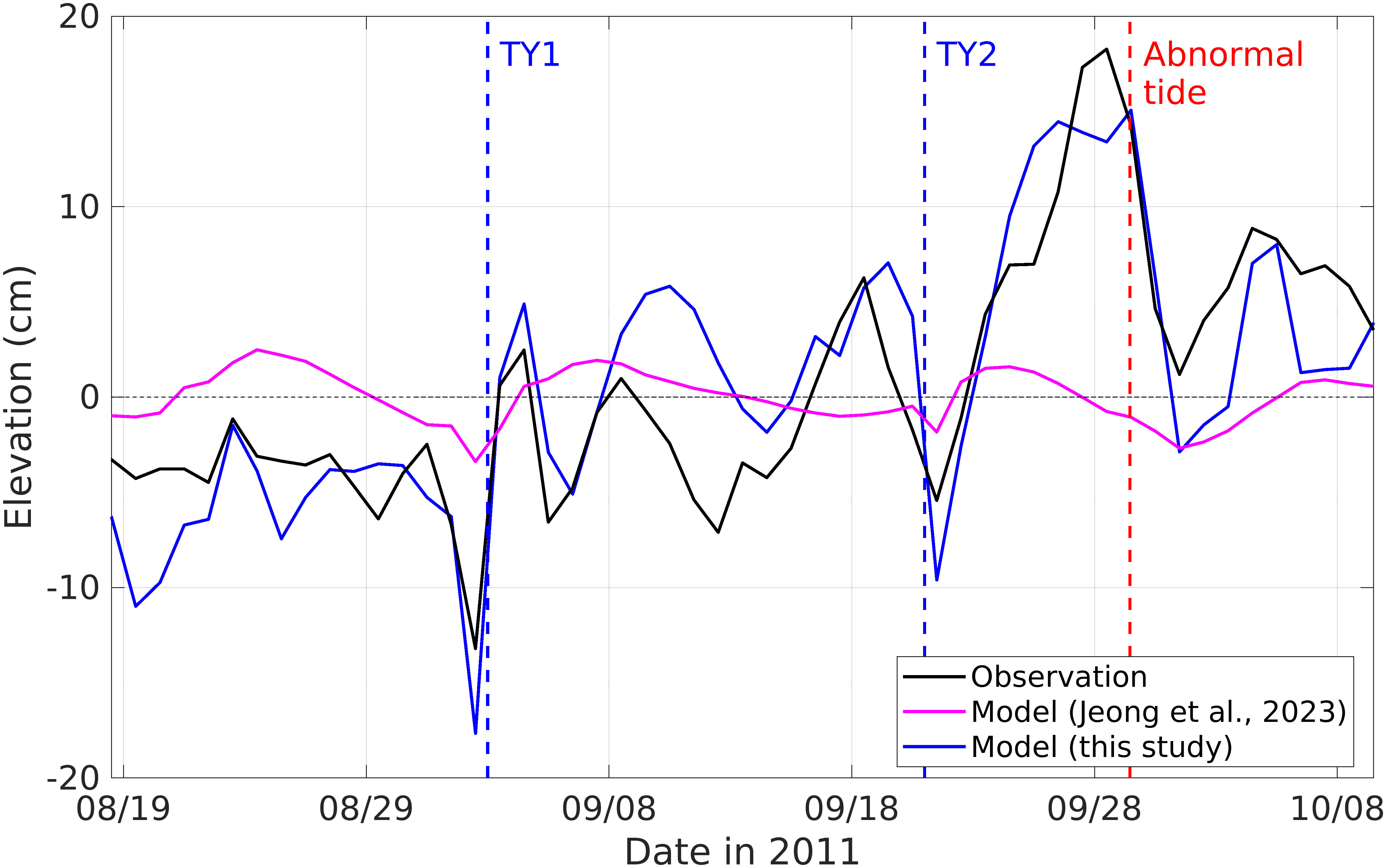
Figure 11 Comparisons of subtidal components from previous observations, previous study (based on data from Jeong et al., 2023), and the present study.

The amplitude and phase of abnormal tides in the eastern region exhibited better performance than did those in the previous literature Usui et al. (2021). For the analysis, they used an operational coastal model of the Seto Inland Sea, MRI.COM-Seto (Sakamoto et al., 2016). The MRI.COM-JPN model used in the present study was developed by expanding the MRI.COM-Seto from the SIS to the entire coastal seas around Japan, introducing explicit tides, etc (Sakamoto et al., 2019). Therefore, the MRI.COM-JPN and MRI.COM-Seto could not capture the signal of abnormal tides because they were kind of siblings. Similarly, as we corrected the open boundary conditions of the SIS model to improve model performance, the MRI.COM-Seto applied four-dimensional variational (4DVAR) data assimilation (Usui et al., 2015). As a result, both the SIS model in this study and the MRI.COM-Seto model yielded reasonable results.

With respect to the open boundary bias correction, the eastern open boundary had a more significant influence on the model results. After applying corrections using differences at the western Hosojima and eastern Shirahama stations, the model performance notably improved, especially at the Shirahama and Osaka stations on the eastern side. However, this ad hoc correction doesn’t involve a systematic analysis or correction of biases within the model but rather replaces modeled values with observed values at specific locations without considering the underlying reasons for discrepancies between model outputs and observations. Thus, proper bias correction methods typically involving more sophisticated statistical techniques that aim to systematically adjust the model outputs to minimize the biases across the entire domain of interest, considering the complex interactions and sources of error within the modeling process, should be considered in future works.

The MAEs at these stations were poor among the six stations before correction. However, these stations showed the best MAEs after correction (see Table 3). The IOAs at these stations were also the highest among the six stations. In contrast, the improvements at the Hosojima and Oita stations on the western side were relatively modest. Suenaga et al. (2003); Usui et al. (2021) suggested that sea level variations can be induced by CTWs propagating from east to west along the eastern land boundary. Similarly, in the present study, the eastern side appears to be a critical area for abnormal tides in Hiroshima Bay.

In hydrodynamic modeling, especially when investigating mass exchanges through straits or similar narrow passages, other types of filtering techniques can be employed besides Shapiro method. Mass filtering techniques are used to control the mass fluxes through certain regions or boundaries in a hydrodynamic model. They are particularly useful in situations where accurate representation of mass exchanges is crucial, such as in simulating flow through straits where water from one basin flows into another, including e.g., the proper definition of mass flux boundaries, adjustment of mass fluxes (usually based on field observations), renormalization techniques in Lagrangian models, weighted-averaging techniques for mass balance, source/sink terms adjustment, boundary condition modification (data-assimilated regulation of mass fluxes), adaptive grid refinement (adjusting spatial resolution of model meshes based on flow characteristics), changing the advection scheme (to accurately capture mass transport phenomena), and numerical filters, such as Shapiro filter, to damp numerical oscillations and stabilize solution processes. In this study, we applied Shapiro filter only and it is worth investigating the effects of various mass filtering techniques in the SIS circulation in future works.

5 Conclusions

The Seto Inland Sea (SIS) is a semienclosed sea located in western Japan with an elliptical shape and a major (minor) axis of approximately 450 km (75 km). The time-averaged sea level distribution in the SIS mostly has a west-high-east-low pattern along the major axis, resulting in continuous easterly throughflow at the center of the SIS. However, in September 2011, two typhoons (TY1 and TY2) approached the SIS and disturbed sea level distributions in the reverse pattern (west low-east high). Another event, an abnormal tide, resulted in a distinct sea level increase in Hiroshima Bay. We investigated the variations in circulation in the SIS when these typhoons and abnormal tides affected the sea surface height distribution.

The SIS circulation was investigated using the SCHISM model for 61 days in the summer of 2011 with SSH bias correction at the open boundary. After the SSH bias correction using the differences in subtidal components between the observations and model results, the SIS model showed much improved results in terms of subtidal components. After the correction, the 6-station-averaged MAE decreased by 6.0 cm from 9.2 cm to 3.2 cm. The average IOA also improved by 0.49 from 0.23 to 0.72.

Net fluxes of seawater at four cross-sections were calculated from the model results before and after the correction to investigate the process inducing the variation in subtidal components. The net flux dominantly determined the total net flux into the SIS through the Bungo Channel. At TY1, the correct model showed no increase in subtidal elevation, although the original model showed a longer and greater peak at all stations. The longer peak (relatively long-term sea level variation) in the SIS was mainly induced by the additional influx at the Bungo Channel. A sharp peak (relatively short-term variation) at TY1 around the Osaka station was caused by a reduction in outflow at the Kii Channel. These results indicate that the influx via the Bungo Channel is key to the subtidal variation in sea level in Hiroshima Bay and the whole SIS. In the case of typhoons, the Kii Channel can affect sea level variation around the Kii Channel more than the Bungo Channel can.

Regarding the circulation in the SIS, the Kii Channel seems to have a more dominant influence than the Bungo Channel. The pattern of the net flux at Harima Nada (center of the SIS) was similar to the inverse pattern of the net flux at the Kii Channel. This means that the outflux of seawater at the Kii Channel needs to take precedence for the generation of flow at the center of the SIS. Although influx from the Bungo Channel was the main source of seawater, the most important factor for circulation was discharge through the Kii Channel.

The Kanmon Strait has a much narrower width than the other two main channels. However, it has the important function of mitigating rapid sea level rise. Seawater inflowed from the Bungo Channel through the strait and discharged steadily despite its slight amount. In the absence of the Kanmon Strait, the sea level can rise faster and be restored more slowly. The order of discharged seawater from the Kanmon Strait was comparable to the amount of river discharge from twenty-two first-class rivers.

Approximately 15% of the amplitude of the abnormal tide in Hiroshima Bay was attributed to internal seiche-induced sea level variation on the scale of Hiroshima Bay. The main cause of the abnormal tide was seawater exchanges through two channels: the Bungo and Kii Channels. In particular, the Bungo Channel was a major contributor to water exchange and sea level variations, especially in the western part of the SIS. Sea level variations in the eastern part were determined by compound impact of the two channels. This study elucidates the effect of circulation in the SIS and the main roles of each channel, strait, and basin on abnormal tides. This process will improve our understanding and knowledge of the SIS and increase our chances of being prepared for natural disasters in the future.

As limitations, the variations of circulation in the SIS were traced only by a model simulation that was corrected to fit to the in situ measured variations of sea level on the boundary. This ad hoc bias correction can cause bias to the actual circulation patterns in the SIS and has to be improved with systematic bias correction method with possible hydrodynamic field measurements or available satellite data in future works. A detailed quantitative process-based study on the role of CTWs, the Kuroshio warm current, the Pacific Oscillation, and the Hiroshima Bay internal seiche in abnormal tides will be performed in our future studies based on field measurements and improved SIS modeling.

Data availability statement

The raw data supporting the conclusions of this article will be made available by the authors, without undue reservation. The observed tides and water temperature used for model validation in the study are retrieved and available via www.jodc.go.jp. The observed river discharges used for input data are available via www1.river.go.jp. The initial and boundary condition data were obtained from the Japanese Coastal Ocean Monitoring and Forecasting System (MRI.COM-JPN) developed by the Meteorological Research Institute (MRI) of the Japan Meteorological Agency (JMA) (available via https://search.diasjp.net/ja/dataset/MOVEJPN_MRI_2020). FES2014 was produced by Noveltis, Legos, and CLS and distributed by Aviso+, with support from CNES (https://www.aviso.altimetry.fr/). The MSM used for meteorological conditions is available at http://database.rish.kyotou.ac.jp/arch/jmadata/data/. ERA5 was retrieved from the Copernicus Climate Change Dataset of the ECMWF and modified by interpolation and calculation for the necessary variables of the SCHISM. These links were valid as of 10 November 2023. MATLAB version R2022a was used for pre- and postprocessing, and author-developed MATLAB codes for data processing and analysis are also available from the authors upon request.

Author contributions

J-SJ: Writing – review & editing, Writing – original draft, Visualization, Validation, Software, Resources, Methodology, Investigation, Formal Analysis, Conceptualization. HL: Writing – review & editing, Writing – original draft, Supervision, Project administration, Methodology, Investigation, Funding acquisition, Formal Analysis, Conceptualization. NM: Writing – review & editing, Project administration, Methodology, Investigation.

Funding

The author(s) declare that financial support was received for the research, authorship, and/or publication of this article. This paper is supported by the collaborative research program (2023GC-03) of the Disaster Prevention Research Institute of Kyoto University.

Conflict of interest

The authors declare that the research was conducted in the absence of any commercial or financial relationships that could be construed as a potential conflict of interest.

Publisher’s note

All claims expressed in this article are solely those of the authors and do not necessarily represent those of their affiliated organizations, or those of the publisher, the editors and the reviewers. Any product that may be evaluated in this article, or claim that may be made by its manufacturer, is not guaranteed or endorsed by the publisher.

References

Bonaduce A., Pinardi N., Oddo P., Spada G., Larnicol G. (2016). Sea-level variability in the Mediterranean Sea from altimetry and tide gauges. Clim. Dyn. 47, 2851–2866. doi: 10.1007/s00382-016-3001-2

CrossRef Full Text | Google Scholar

Carrère L., Lyard F. H., Cancet M., Guillot A. (2015). FES 2014, a new tidal model on the global ocean with enhanced accuracy in shallow seas and in the Arctic region. in EGU General Assembly Conference Abstracts, vol. 17, p. 5481.

Google Scholar

Chang P.-H., Guo X., Takeoka H. (2009). A numerical study of the seasonal circulation in the Seto Inland Sea, Japan. J. Oceanogr. 65, 721–736. doi: 10.1007/s10872-009-0062-4

CrossRef Full Text | Google Scholar

Cowles G. W., Lentz S. J., Chen C., Xu Q., Beardsley R. C. (2008). Comparison of observed and model-computed low frequency circulation and hydrography on the New England Shelf. J. Geophys. Res. Ocean. 113, 1–17. doi: 10.1029/2007JC004394

CrossRef Full Text | Google Scholar

Dou Y., Li J., Zhao J., Wei H., Yang S., Bai F., et al. (2014). Clay mineral distributions in surface sediments of the Liaodong Bay, Bohai Sea and surrounding river sediments: Sources and transport patterns. Cont. Shelf Res. 73, 72–82. doi: 10.1016/j.csr.2013.11.023

CrossRef Full Text | Google Scholar

Hersbach H., Bell B., Berrisford P., Hirahara S., Horányi A., Muñoz-Sabater J., et al. (2020). The ERA5 global reanalysis. Q. J. R. Meteorol. Soc 146, 1999–2049. doi: 10.1002/qj.3803

CrossRef Full Text | Google Scholar

Hirose N., Usui N., Sakamoto K., Tsujino H., Yamanaka G., Nakano H., et al. (2019). Development of a new operational system for monitoring and forecasting coastal and open-ocean states around Japan. Ocean Dyn. 69, 1333–1357. doi: 10.1007/s10236-019-01306-x

CrossRef Full Text | Google Scholar

Hughes C. W., Fukumori I., Griffies S. M., Huthnance J. M., Minobe S., Spence P., et al. (2019). Sea level and the role of coastal trapped waves in mediating the influence of the open ocean on the coast. Surv. Geophys. 40, 1467–1492. doi: 10.1007/s10712-019-09535-x

CrossRef Full Text | Google Scholar

Jeong J.-S., Lee H. S. (2023). Unstructured grid-based river-coastal ocean circulation modeling towards a digital twin of the Seto inland sea. Appl. Sci. 13, 8143. doi: 10.3390/app13148143

CrossRef Full Text | Google Scholar

Jeong J.-S., Lee H. S., Mori N. (2023). Abnormal high tides and flooding induced by the internal surge in Hiroshima Bay due to a remote typhoon. Front. Mar. Sci. 10. doi: 10.3389/fmars.2023.1148648

CrossRef Full Text | Google Scholar

Jeong J. S., Woo S. B., Lee H. S., Gu B. H., Kim J. W., Song J. (2022). Baroclinic effect on inner-port circulation in a macro-tidal estuary: A case study of Incheon North Port, Korea. J. Mar. Sci. Eng. 10, 392. doi: 10.3390/jmse10030392

CrossRef Full Text | Google Scholar

Khangaonkar T., Long W., Xu W. (2017). Assessment of circulation and inter-basin transport in the Salish Sea including Johnstone Strait and Discovery Islands pathways. Ocean Model. 109, 11–32. doi: 10.1016/j.ocemod.2016.11.004

CrossRef Full Text | Google Scholar

Kurogi M., Hasumi H. (2019). Tidal control of the flow through long, narrow straits: a modeling study for the Seto Inland Sea. Sci. Rep. 9, 11077. doi: 10.1038/s41598-019-47090-y

PubMed Abstract | CrossRef Full Text | Google Scholar

Kwak M.-T., Cho Y.-K. (2020). Seasonal variation in residence times of two neighboring bays with contrasting topography. Estuaries Coasts 43, 512–524. doi: 10.1007/s12237-019-00644-9

CrossRef Full Text | Google Scholar

Laurel-Castillo J. A., Valle-Levinson A. (2020). Tidal and subtidal variations in water level produced by ocean-river interactions in a subtropical estuary. J. Geophys. Res.: Oceans 125, e2018JC014116. doi: 10.1029/2018JC014116

CrossRef Full Text | Google Scholar

Lee H. S., Shimoyama T., Popinet S. (2015). Impacts of tides on tsunami propagation due to potential Nankai Trough earthquakes in the Seto Inland Sea, Japan. J. Geophys. Res. Ocean. 120, 6865–6883. doi: 10.1002/2015JC010995

CrossRef Full Text | Google Scholar

Nakatani Y., Tomura Y., Nishida S. (2020). Analysis of ocean water behavior in the Seto Inland Sea and the Pacific Ocean region using an unstructured grid model. J. Japan Soc. Civ. Eng. Ser. B2 (Coastal Eng.) 76, 997–1002. doi: 10.2208/kaigan.76.2_I_997

CrossRef Full Text | Google Scholar

Patgaonkar R. S., Vethamony P., Lokesh K. S., Babu M. T. (2012). Residence time of pollutants discharged in the Gulf of Kachchh, northwestern Arabian Sea. Mar. pollut. Bull. 64, 1659–1666. doi: 10.1016/j.marpolbul.2012.05.033

PubMed Abstract | CrossRef Full Text | Google Scholar

Payandeh A. R., Justic D., Mariotti G., Huang H., Sorourian S. (2019). Subtidal water level and current variability in a bar-built estuary during cold front season: Barataria bay, gulf of Mexico. J. Geophys. Res.: Oceans 124, 7226–7246. doi: 10.1029/2019JC015081

CrossRef Full Text | Google Scholar

Pinardi N., Bonaduce A., Navarra A., Dobricic S., Oddo P. (2014). The mean sea level equation and its application to the Mediterranean sea. J. Clim. 27, 442–447. doi: 10.1175/JCLI-D-13-00139.1

CrossRef Full Text | Google Scholar

Sagawa N., Kawaai K., Hinata H. (2018). Abundance and size of microplastics in a coastal sea: Comparison among bottom sediment, beach sediment, and surface water. Mar. pollut. Bull. 133, 532–542. doi: 10.1016/j.marpolbul.2018.05.036

PubMed Abstract | CrossRef Full Text | Google Scholar

Saito K., Fujita T., Yamada Y., Ishida J., Kumagai Y., Aranami K., et al. (2006). The operational JMA nonhydrostatic mesoscale model. Mon. Weather Rev. 134, 1266–1298. doi: 10.1175/MWR3120.1

CrossRef Full Text | Google Scholar

Sakamoto K., Tsujino H., Nakano H., Urakawa S., Toyoda T., Hirose N., et al. (2019). Development of a 2-km resolution ocean model covering the coastal seas around Japan for operational application. Ocean Dyn. 69, 1181–1202. doi: 10.1007/s10236-019-01291-1

CrossRef Full Text | Google Scholar

Sakamoto K., Yamanaka G., Tsujino H., Nakano H., Urakawa S., Usui N., et al. (2016). Development of an operational coastal model of the Seto Inland Sea, Japan. Ocean Dyn. 66, 77–97. doi: 10.1007/s10236-015-0908-9

CrossRef Full Text | Google Scholar

Shapiro R. (1970). Smoothing, filtering, and boundary effects. Rev. Geophys. 8, 359–387. doi: 10.1029/RG008i002p00359

CrossRef Full Text | Google Scholar

Suenaga M., Matsumoto H., Itahashi N., Mihara M., Umeki Y., Isobe M. (2003). About abnormal tide level in Hiroshima Bay. Proc. Coast. Eng. Japan Soc Civ. Eng. 50, 1316–1320. doi: 10.2208/proce1989.50.1316

CrossRef Full Text | Google Scholar

Takagi H., Esteban M., Mikami T., Fujii D. (2016). Projection of coastal floods in 2050 Jakarta. Urban Clim. 17, 135–145. doi: 10.1016/j.uclim.2016.05.003

CrossRef Full Text | Google Scholar

Usui N., Fujii Y., Sakamoto K., Kamachi M. (2015). Development of a four-dimensional variational assimilation system for coastal data assimilation around Japan. Mon. Weather Rev. 143, 3874–3892. doi: 10.1175/MWR-D-14-00326.1

CrossRef Full Text | Google Scholar

Usui N., Ogawa K., Sakamoto K., Tsujino H., Yamanaka G., Kuragano T., et al. (2021). Unusually high sea level at the south coast of Japan in September 2011 induced by the Kuroshio. J. Oceanogr. 77, 447–461. doi: 10.1007/s10872-020-00575-1

CrossRef Full Text | Google Scholar

Willmott C. J. (1981). ON THE VALIDATION OF MODELS. Phys. Geogr. 2, 184–194. doi: 10.1080/02723646.1981.10642213

CrossRef Full Text | Google Scholar

Willmott C. J. (2005). Advantages of the mean absolute error (MAE) over the root mean square error (RMSE) in assessing average model performance. Clim. Res. 30, 79–82. doi: 10.3354/cr030079

CrossRef Full Text | Google Scholar

Willmott C. J., Robeson S. M., Matsuura K. (2012). A refined index of model performance. Int. J. Climatol. 32, 2088–2094. doi: 10.1002/joc.2419

CrossRef Full Text | Google Scholar

Woodworth P. L., Melet A., Marcos M., Ray R. D., Wöppelmann G., Sasaki Y. N., et al. (2019). Forcing factors affecting sea level changes at the coast. Surv. Geophys. 40, 1351–1397. doi: 10.1007/s10712-019-09531-1

CrossRef Full Text | Google Scholar

Yanagi T., Takeoka H., Tsukamoto H. (1982). Tidal energy balance in the Seto Inland Sea. J. Oceanogr. Soc Japan 38, 293–299. doi: 10.1007/BF02114533

CrossRef Full Text | Google Scholar

Zhang B., Pu A., Jia P., Xu C., Wang Q., Tang W. (2021). Numerical simulation on the diffusion of alien phytoplankton in Bohai bay. Front. Ecol. Evol. 9. doi: 10.3389/fevo.2021.719844

CrossRef Full Text | Google Scholar

Zhang Y., Baptista A. M. (2008). SELFE: A semi-implicit Eulerian–Lagrangian finite-element model for cross-scale ocean circulation. Ocean Model. 21, 71–96. doi: 10.1016/j.ocemod.2007.11.005

CrossRef Full Text | Google Scholar

Zhang Y. J., Fernandez-Montblanc T., Pringle W., Yu H.-C., Cui L., Moghimi S. (2023). Global seamless tidal simulation using a 3D unstructured-grid model (SCHISM v5.10.0). Geosci. Model. Dev. 16, 2565–2581. doi: 10.5194/gmd-16-2565-2023

CrossRef Full Text | Google Scholar

Zhang C., Kaneko A., Zhu X., Lin J. (2014). Nontidal sea level changes in Hiroshima Bay, Japan. Acta Oceanol. Sin. 33, 47–55. doi: 10.1007/s13131-014-0516-4

CrossRef Full Text | Google Scholar

Zhang Y. J., Stanev E. V., Grashorn S. (2016). Unstructured-grid model for the North Sea and Baltic Sea: Validation against observations. Ocean Model. 97, 91–108. doi: 10.1016/j.ocemod.2015.11.009

CrossRef Full Text | Google Scholar

Appendix

Figure A1

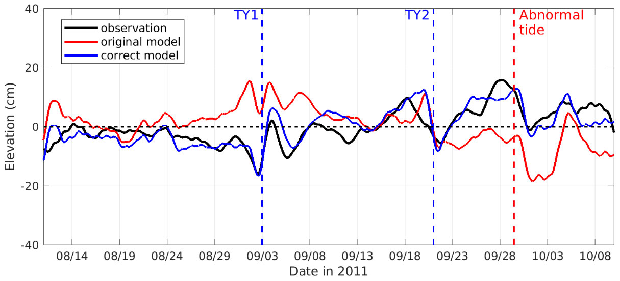
Figure A1 Subtidal elevations at Kure station calculated by T-Tide software and 1 day low-pass filter. T_Tide and T_Predic were applied to remove tidal signal, then the low-pass filter was applied to remove high-frequency noises. This results at Kure station do not show significant difference with the daily averaged values in Figure 8A.