A dissolved oxygen prediction model based on GRU–N-Beats

1 Introduction

In order to provide a cultural environment suitable for fish growth, it is important to test the water quality. Dissolved oxygen is an important indicator representing the oxygen content in water, and the amount of dissolved oxygen required varies slightly for different fish species. In aquaculture, the amount of dissolved oxygen in the water often fluctuates due to changes in the aquatic environment. The lack of dissolved oxygen often leads to the floating head of fish or even death. At the same time, high dissolved oxygen levels cause harm to fish, such as bubble disease, which is caused by the lack of sufficient aeration of dissolved oxygen in the water following prolonged direct sunlight (Zhou et al., 2021). Too high or too low dissolved oxygen leads to disease or death of fish, which will cause irreversible economic losses. Due to environmental changes, the amount of dissolved oxygen in the same pond varies at different times of the day (Cao et al., 2020), with dissolved oxygen levels often the highest at noon and the lowest in the evening. In fish ponds, microorganisms, animals, and plants form a mini-ecosystem, and different organisms require different dissolved oxygen levels. Influenced by the environment, climate, aquatic organisms, and human behavior, dissolved oxygen content often shows a non-linear trend (Ta and Wei, 2018). Therefore, accurate dissolved oxygen prediction in this aquaculture environment poses a significant challenge. Accurate prediction of dissolved oxygen in the water and advanced control of oxygenators can help increase fishery production, improve efficiency, and reduce costs (Cao X. et al., 2021).

Due to the complex environment of aquaculture, the data collected by sensors are often affected by multiple factors, thus causing noise problems in the collected samples. Ren et al. (2020) used variational mode decomposition to decompose dissolved oxygen data to obtain signals of different frequencies, thus reducing noise and getting higher prediction accuracy. Zhang et al. (2020) used kernel principal component analysis (KPCA) for feature selection of water quality data in Australian river data to minimize the effect of water quality noise on model training. They used recurrent neural network (RNN) with temporal memory function (Hu et al., 2021) to predict the water quality parameter with Feedforward Neural Network (FFNN), Support Vector Regression (SVR), and Generalized Regression Neural Network (GRNN). These methods were compared, and it was proved that RNN was more advantageous for processing time-series data. Li et al (Li et al., 2022). pointed out that the multivariate and long-term correlation characterizing water quality time series in traditional methods makes it difficult to achieve the desired prediction accuracy. To address this issue, they combined long short-term memory (LSTM) and temporal convolutional network (TCN) to construct a prediction model and also investigated the effects of attention mechanisms and historical time window size on prediction results. Ni et al (Ni et al., 2023). introduced a deep learning model, Fast Graph Convolutional Networks (FTGCN), to predict multivariable water quality data, enhancing prediction accuracy by capturing potential correlations, temporal dependencies, and hidden associations between indicators. Liu et al (Liu et al., 2023). proposed a novel prediction framework for effluent total nitrogen (E-TN) in wastewater treatment plants (WWTPs), combining a two-stage feature selection model, Golden Jackal Optimization (GJO) algorithm, and a hybrid deep learning model convolutional neural network (CNN)–LSTM–TCN (CLT). The framework effectively captures non-linear relationships in multivariate time series. Zamani et al (Zamani et al., 2023). evaluated the predictive capabilities of four deep learning models in forecasting chlorophyll-a concentrations in Small Prespa Lake, Greece. The best-performing model, gated recurrent unit (GRU), is further enhanced through ensemble modeling with genetic algorithms.

In time-series prediction studies, it is a common practice to divide the one-dimensional dissolved oxygen data by time steps and use the obtained multiple small time series as training data to perform the prediction. However, the amount of dissolved oxygen in recirculating aquaculture is often affected by a variety of environmental factors, and the mechanism of this action is very complex. Accurate predictions cannot be made by a single dissolved oxygen data, such as the electrical conductivity of the water body, pH, and ammonia nitrogen concentration. Since one-dimensional time series usually contain only continuous data points for a single variable and lack diverse sources of information, their forecasting accuracy is often severely limited. One-dimensional time-series data is characterized by the fact that it reflects only the pattern of change in a particular indicator over time and fails to encompass other factors that may affect the change in that indicator. This data limitation leads to the limited ability of models to capture complex patterns, trends, and unexpected events, which in turn affects the accuracy and reliability of forecasts. Therefore, with the development of artificial intelligence technology, multidimensional time-series prediction techniques have been proposed. Many scholars from China Agricultural University have conducted multiple in-depth research on multivariate dissolved oxygen prediction in aquaculture. Liu (2019) proposed a recurrent neural network based on a self-attentive mechanism. Zhou et al. (2022) predicted dissolved oxygen in aquaculture by an improved sparrow search algorithm (Yang et al., 2021).

Early time-series prediction studies mainly used statistical methods [including Autoregression (AR), Moving Average (MA), Auto-Regressive Moving Average (ARMA), Autoregressive Integrated Moving Average (ARIMA), and Seasonal Autoregressive Integrated Moving Average (SARIMA)], which have the advantages of simple training, fast speed, and good interpretability. In practical scenarios, since the trend of dissolved oxygen is often non-linear and fluctuates along with environmental factors, it is difficult for traditional mathematical models to describe its change process, while artificial intelligence methods can better solve problems such as non-linear prediction. Therefore, artificial intelligence methods are now the development trend. Currently, an effective method is to predict the time-series data by neural networks, such as back-propagation (BP) neural network, extreme learning machine (ELM) (Kuang et al., 2020), radial basis neural network (RBNN) (Li et al., 2021), and CNN (Cao S. et al., 2021). Cao et al. (2020) used an attention mechanism and GRU based on the difference of dissolved oxygen in a pond on a three-dimensional scale to predict the dissolved oxygen in the center of the pond. Trained gradient-boosted regression tree (GBRT) by a stochastic search algorithm was used to construct a set of deep neural networks capable of predicting any location in the pond. In addition, they proposed a GRU model, clustered dissolved oxygen data using the K-means algorithm, and trained the data similarity around dissolved oxygen. Li et al. (2022) proposed a causal convolution and jump convolution of time series using LSTM and TCN to process long time series.

The feature extraction network, GRU, used in this paper is an improved network based on RNN and LSTM networks. It overcomes to some extent the problem of memory loss in RNN when dealing with long sequences and the problem of complex structure and time overhead of LSTM. GRU can deal with multidimensional time series and combine various water quality information in the water body for prediction, so it is higher in prediction accuracy than previous one-dimensional prediction models. This paper used GRU for feature extraction and combined it with the N-Beats network. Oreshkin et al. (2020) used it to predict dissolved oxygen. These algorithms provide the theoretical basis for the research in this paper. There are three main problems in dissolved oxygen prediction: first, data are missing issues in water quality sensor data acquisition and transmission; second, the coupling mechanism between the data is complicated; and third, the stability and reliability of the traditional methods are poor. In order to solve these problems, this paper preprocessed the data and took the feature extraction and N-Beats prediction. First, N-Beats is based on forward and backward residual networks for layer-by-layer learning, which makes it possible to train the target data quickly without complicated changes when facing new samples. In addition, the N-Beats network is built with a Block structure, and sequence decomposition can fully explain each part’s prediction results. Finally, since the learning process of the residual network is based on one-level operations, the prediction speed is fast, which is of great significance for the real-time prediction of dissolved oxygen and immediate control of equipment in complex aquaculture environments (Sun et al., 2021). The main work of this paper is as follows.

(1) To solve the problem of dissolved oxygen prediction in aquaculture, an improved multidimensional time-series prediction model based on the N-Beats network was proposed in this paper to reduce the economic loss due to the time lag of equipment control in actual production (Zhang and Wu, 2020).

(2) Various time-series prediction models were compared and analyzed, and experiments demonstrated that the algorithm in this paper has better stability and prediction accuracy.

(3) The problem that N-Beats cannot handle multidimensional time series was solved. To prevent overfitting, this paper used the Dropout algorithm to improve the generalization ability of the model.

(4) The algorithm in this paper has strong explanatory power and improves the model’s ability to handle data from different scenes.

2 Materials and methods

2.1 System structure

This paper proposed a multivariate temporal prediction model for the dissolved oxygen content in ponds in aquaculture (Huang et al., 2021). The method in this paper consists of three processes: preprocessing, feature extraction, and dissolved oxygen prediction. Combined with the N-Beats network, we took the residuals of each step as input, used multiple blocks for learning, and finally superimposed the fitting results of each block to get the final prediction results. The network structure is shown in Figure 1.

Figure 1

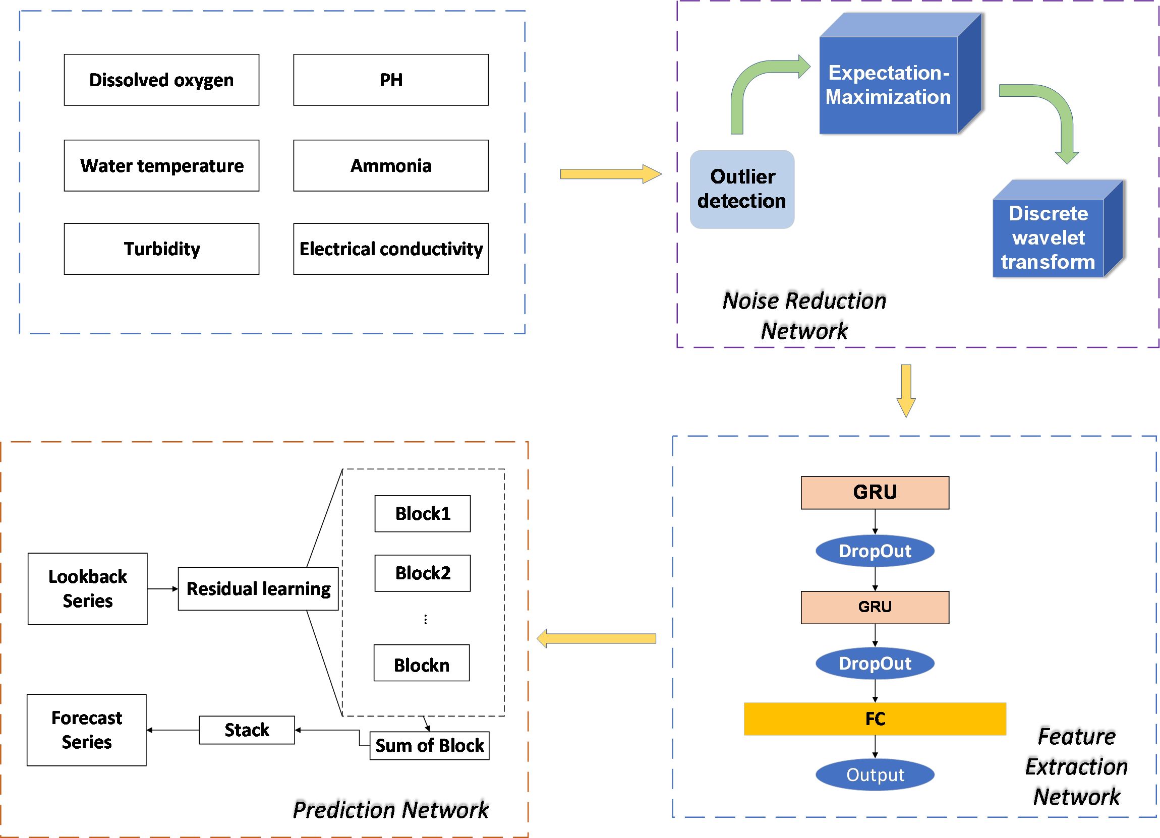
Figure 1 Overall network architecture diagram.

The network in this paper contains the following three main processing processes.

(1) The raw data collected by the farming system include six sets of data: water temperature, pH, ammonia and nitrogen concentration, turbidity, electrical conductivity, and dissolved oxygen. The data were first fed into the noise reduction module to detect outliers of the original data and fill in the missing values by fitting them using the expectation–maximization (EM) algorithm. After that, the overall sample was noise-reduced by wavelet transform in the noise reduction network to reduce the errors generated by the sensor in data acquisition and transmission.

(2) The processed time series in (1) was passed through the GRU module for feature extraction. The advantages of GRU are mainly as follows. First, the temporal feature extraction network can extract the variation characteristics of the time series in both temporal and spatial dimensions from multiple dimensions. Second, the feature extraction network based on the gated recurrent unit is more advantageous than the LSTM network in handling large batches of temporal data, which can significantly reduce the training time of the model while ensuring the accuracy of the prediction (Feng et al., 2020). The six kinds of water quality information were passed through the GRU module to adjust the parameter states between the hidden layers. After this, a fully connected layer merged the six water quality information for input to the N-Beats network.

(3) In the third module, the output of the feature extraction network was used as the input of the prediction network, and the sequences were divided into forecast and lookback input Blocks, where the forecast is the prediction sequence and lookback is the lookback window sequence. In addition, in order to reflect the interpretability of the model, the data were decomposed into seasonal and trend data to explain the final prediction results (seasonal data explain the model results in terms of periodicity, while trend data portray the trend of dissolved oxygen changes in the future period). The results of each Block were output by calculating the residuals from the output of the previous Block with itself, and the results of different Blocks were superimposed to obtain the final prediction results.

2.2 Data preprocessing

In the aquaculture workshop, six water quality sensors were configured to collect six types of data: dissolved oxygen, ammonia, nitrogen concentration, water temperature, conductivity, pH, and turbidity. Sensors used for field data acquisition may be interfered by a variety of factors, due to the complex site environment, sensor equipment failure, and even the data transmission process, the signal interference is produced, so the collected data often face large deviations, missing data, and other problems. In this subsection, this paper will accomplish the filling of data vacancy values and the replacement of outliers for various problems in the original dataset by using the EM algorithm. In addition, to reduce the problem of noise in the samples, this paper used the discrete wavelet transform (DWT) to decompose the original signals and remove the redundant signals, thus ensuring the prediction accuracy of the subsequent model.

2.2.1 Expectation–maximization algorithm

In the aquaculture environment, due to uncertainty factors such as the instability of signal transmission and the field environment, the anomalous data are first detected and set to null values. Then, the missing values are estimated using the EM algorithm. This section describes in detail the principle of the EM algorithm.

Initially proposed in 1977 by Arthur P. Dempster, Nan Laird, and Donald Rubin (Simone, 2021), the EM algorithm is an algorithm for parameter optimization through iteration. The basic idea of the EM algorithm is to predict the missing data by fitting the estimated parameters and using the predicted results as new data for re-estimation, after which iterations are repeated until the model converges and the final result is obtained (Zhao et al., 2020).

$\begin{array}{ll}\begin{array}{c}\ell (\theta |X)=\log P(X|\theta )\\ =\log \left(\prod _{i=1}^{n}P(x_i|\theta )\right)\\ =\sum _{i=1}^n\log P(x_i|\theta )\end{array}& (1)\end{array}$

As shown in Equation (1), L is the joint probability distribution of X, as shown in Equation (2), where $\theta$ is the parameter to estimate the missing water quality data. In order to find the optimal solution, the derivative of Equation (1) was performed to obtain the maximum likelihood function (Zhao et al., 2018).

$\begin{array}{ll}\begin{array}{c}\widehat{\theta }=\arg \underset{\theta }{\max }\log \ell (\theta |X)\\ =\arg \underset{\theta }{\max }\sum _{i=1}^n\log P(x_i|\theta )\end{array}& (2)\end{array}$

As shown in Equation (3), for time series $X=(x_1,x_2,\dots ,x_n)$, its expectation is $E[X]=\sum _{}xP(x)$, the sequence of unobserved hidden variables is $z=(z_1,z_2,\dots ,z_n)$, and the hidden variables satisfy $\sum _{Z}q(Z)=1$, at which point it is obtained that

$\begin{array}{ll}\begin{array}{c}\log P(X|\theta )=\log \sum _{Z}P(X,Z|\theta )\\ =\log \left(\sum _{Z}P(X|\theta ,Z)P(Z|\theta )\right)\end{array}& (3)\end{array}$

Because the dissolved oxygen data change curve over time is a concave or convex function, according to Jensen’s inequality, the mathematical expectation of the convex function must be greater than or equal to its function value, and the following equation can be obtained.

$\begin{array}{ll}E[f(X)]\ge f(E[X])& (4)\end{array}$

In this equation, $X$ is a random variable. It is a convex function, and Equation (4) takes an equal sign when and only when it is a constant (Xiao and Lu, 2020). If it is a concave function, the inequality sign is reversed. From this, Equation (5) can be obtained.

$\begin{array}{ll}{E}_Z\left[\log \frac{P(X,Z|\theta )/q(Z)}{P(Z|X,\theta )/q(Z)}\right]\ge \sum _{Z}q(Z)\log \frac{P(X,Z|\theta )}{q(Z)}& (5)\end{array}$

As shown in Equation (6), the maximum likelihood function is

$\begin{array}{ll}\widehat{\theta }=\arg {\max }_{\theta }{E}_{Z|X,{\theta }^{(i)}}[\log P(X,Z|\theta )]& (6)\end{array}$

As shown in Equation (7), the expectation of the joint probability distribution is obtained as

$\begin{array}{ll}\begin{array}{c}Q\left(\theta ,{\theta }^{(i)}\right)={\mathbb{E}}_{Z|X,{\theta }^{(i)}}[\log P(X,Z|\theta )]\\ \end{array}& (7)\end{array}$

As shown in Equation (8), bringing the $\theta$ of step i +1 into step i, the equation for step M is obtained as

$\begin{array}{ll}{\theta }^{(i+1)}=\arg \underset{\theta }{\max }Q\left(\theta ,{\theta }^{(i)}\right)& (8)\end{array}$

After obtaining the formulae for the E and M steps, the model converges by taking the water quality information as input for N iterations of E and M. The fitted missing data are obtained when the absolute value between the parameter ${\theta }_{n+1}$ for the N + 1th iteration and the parameter ${\theta }_n$ for the Nth iteration is less than the constant $ϵ$.

The specific algorithm for missing value filling by the EM algorithm is shown in Figure 2.

Figure 2

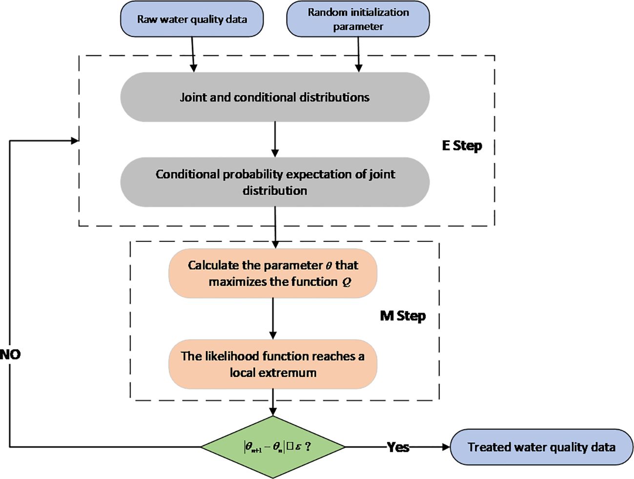
Figure 2 EM algorithm. EM, expectation–maximization.

2.2.2 Wavelet transform

After the EM algorithm fills the missing dissolved oxygen data, although the data have been completely replenished, the noise problem will still arise during the sensor signal acquisition, which will influence the prediction results of the subsequent dissolved oxygen model. Here, we used the wavelet transform method to remove the noise, and the wavelet transform was mainly divided into two stages: signal decomposition and signal reconstruction.

The wavelet transform (WT) discards the disadvantage of the Fourier basis function, which does not perceive the frequency change in the time dimension due to a single variable. In addition, compared to the short-time Fourier transform (STFT) algorithm with adding a window, which generates increased redundancy due to the sine wave in the window during the orthogonalization calculation with the original signal, the wavelet transform proposes a new basis function $a$ and $\tau$ by using these two parameters, $a$ and $\tau$, to perceive the changes of the signal in both frequency and time domains (Sang, 2013). The discrete wavelet transform is given in Equation (9), and the continuous wavelet transform formula is given in Equation (10).

$\begin{array}{ll}{W}_f(j,l,m)=2^j{\int }_{-\mathrm{\infty }}^{+\mathrm{\infty }} {\int }_{-\mathrm{\infty }}^{+\mathrm{\infty }} f(x,y){\psi }^{*}(2^{j}x-l,2^{j}y-m)dxdy& (9)\end{array}$

$\begin{array}{ll}WT(a,\tau )=\frac{1}{\sqrt{a}}{\int }_{-\infty }^{\infty }f(t)*\psi \left(\frac{t-\tau }{a}\right)dt& (10)\end{array}$

The parameter $a$ was used to control the scaling state of the wavelet function, which is used to match the bands of different frequencies, and $\tau$ was used to realize the translation function of the bands to ensure that the wavelet can complete the conversion of the whole frequency band.

To facilitate computer processing and consider the discrete nature of dissolved oxygen data, the wavelet transform needs to use its discrete form, as shown in Equation (11).

$\begin{array}{ll}{W}_f(j,k)=a_0^{-j/2}\psi (a_0^{-j}t-{\tau }_{0}k)& (11)\end{array}$

According to the wavelet transform, the energy $M(\tau )$ of the wavelet is as shown in Equation (12).

$\begin{array}{ll}M(\tau )=\frac{1}{a}\int {\left|W_f(a,\tau )\right|}^{2}d\tau & (12)\end{array}$

The wavelet transform maps the signal to a new variable space by changing different bands of the spectrum, but the energy contained in the same spectrum at the same time before and after the transform is the same as $M(\tau )$.

The water quality data are used as the input of the wavelet transform. The wavelet function is used to transform the original signal through the discrete form of the wavelet transform formula and to ensure that the amount of information contained in the wavelet before and after the transformation is the same. The transformed abnormal signal is rejected through the threshold. Finally, the five components after processing are reconstructed to obtain the noise reduction data as the input of the next network.

2.3 Feature extraction network

Since prediction networks cannot handle multidimensional variables directly, this paper designed a multivariate feature extraction network based on gated recurrent units to extract water quality features. The features were fused through a fully connected neural network as the input to the N-Beats network.

Traditional neural networks ignore the relationship between internal nodes in the same layer because they only construct the information transfer structure between each hidden layer with full connectivity between layers. This structure lacks the feedback between neurons and thus is very difficult to capture the temporal features of long sequences. Based on the characteristics of temporal data, RNNs can obtain temporal memory by constructing information associations between internal neurons, but due to the gradient explosion/disappearance problem of its parameter updates, it often fails to converge to the global optimal solution.

The LSTM has three gates (forgetting gate, memory gate, and output gate) to control the output of cell states. The forgetting gate determines how much of the previous layer’s output is retained by the LSTM, while the memory gate controls how much new information is deposited into the cell state by the current gate. The final output gate then determines the current output value based on the cell state. From the computational process, the add-and-multiply feature of the LSTM reduces the gradient problem caused by the continuous use of linear transformation by RNN.

There are two problems with these methods:

(1) LSTM has three gates, each with a more complex computational process and a larger number of parameters, and it has a longer processing time compared to RNN. This is unacceptable in an actual recirculating water farming workshop, where dissolved oxygen may not be accurately predicted for a longer length of time (Rahman et al., 2020). The complex internal structure of the LSTM may impact the actual production due to the inherent time lag of intelligent remote control.

(2) Each cell of LSTM contains four fully connected layers, which leads to a larger computational volume and requires more computational resources.

By comparing RNN, LSTM, and GRU, this paper chose a GRU as the main structure of the feature extraction network. GRU has a simpler internal structure, smaller computation, and faster computation speed compared with LSTM, and at the same time, the difference between prediction accuracy and LSTM is very small.

The internal structure of the GRU is shown in Figure 3.

Figure 3

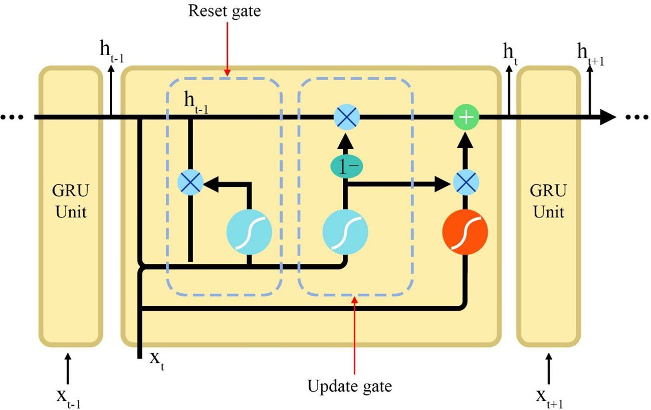
Figure 3 The internal structure of the GRU. GRU, gated recurrent unit.

GRU is another variant of RNN that contains only two gates: the reset gate and the update gate.

First, the update gate is used to compute the newly generated cell state of the current GRU cell. The matrix (donated as W) is obtained by taking the output of the update gate of the previous GRU cell as the current input and then combining it with the input of the current time step. The output is obtained through the activation function after the fully connected layer, and the variable represents the amount of memory that the current GRU cell needs to select from the current calculation result. Equation (13) gives the calculation process.

$\begin{array}{ll}{Z}_t=\sigma (W_z{x}_t+U_z{h}_{t-1}+b_z)& (13)\end{array}$

The update process for the reset gate is shown in Equation (14).

$\begin{array}{ll}{r}_t=\sigma (W_r{x}_t+U_r{h}_{t-1}+b_r)& (14)\end{array}$

$r_t$ is the output of the update gate, $\sigma$ represents the activation function, $W_r$ is the fully connected layer designed for the reset gate, and $h_{t-1}$ and $x_t$ represent the output of the previous time step and the input of the current time step, respectively. $U_r$ is the transition matrix of the reset gate at t − 1 time steps, and $b_r$ is the bias term of the reset gate.

In the reset gate, the matrix $E_r$ is obtained from the output of the previous layer and the current input, and the $E_r$ is passed through the fully connected layer to obtain the output $r_t$.

In the tth time step, the vectors $r_t$ and $h_{t-1}$ are linearly transformed and reconstructed with the tth component of the input sequence, and the features are inner-produced after the fully connected layer. As shown in Equation (15), the current memory content ${\tilde{h}}_t$ is obtained after the activation function.

$\begin{array}{ll}{\tilde{h}}_t=\text{tanh}(W_c{x}_t+U(r_t{h}_{t-1})+b_h)& (15)\end{array}$

Finally, the amount of current memory content to be retained is controlled by the result of the update gate, while the other part determines the proportion of GRU’s memory content retained in the past time series by the output of the hidden layer of the previous time step and the inner product of the vectors. Equation (16) expresses this calculation process:

$\begin{array}{ll}{h}_t=(1-z_t)\ast h_{t-1}+z_t\ast {\tilde{h}}_t& (16)\end{array}$

Where $h_t$ is the output of the hidden layer at the current time step, and $z_t$ is the result of the update gate, which determines the amount of past and current memory content to be saved. The vector $h_{t-1}$ is the output of the previous time step, and ${\tilde{h}}_t$ is the output of the update gate.

Before calculating the dissolved oxygen data of multidimensional variables, since the traditional N-Beats network cannot process multivariate data at the same time, this paper chose to use six GRU modules to extract features from water quality data in turn (Kim et al., 2021). First, the amount of input information saved was controlled using the gating mechanism of GRU, and the saved information from the previous time step was calculated. The update gate added up these two parts of information, after which the output of the current time step was obtained through the activation function. Finally, six sets of output vectors were obtained, and the outputs of the six GRU networks were concatenated. Before inputting into the prediction network, the method in this paper controlled the output dimension through a fully connected neural network. The obtained components were used as the input to the prediction network.

2.4 Prediction network

2.4.1 Residual network

After the feature extraction by the feature network, the six kinds of water quality information in the time dimension were extracted. In the prediction network, an N-Beats network based on residual learning was used in this paper, which can provide a reasonable interpretation of the prediction results because the N-Beats network can decompose the series into trend and seasonality in the time dimension.

Currently, N-Beats is less used in agriculture, but on many publicly available datasets, N-Beats shows great advantages due to its simple structure, strong interpretation, and high operational efficiency. N-Beats mainly consists of a double residual network and a base Block. The internal structure of each Stack is shown in Figure 4.

Figure 4

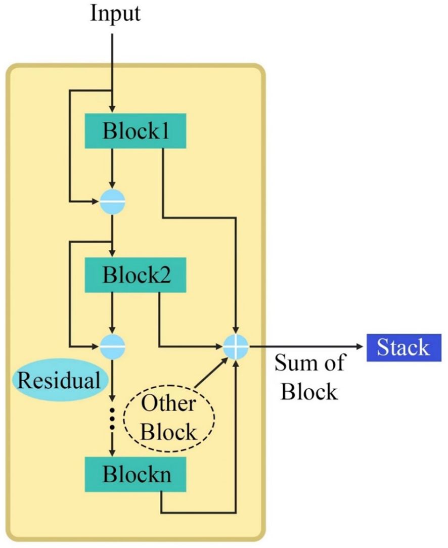
Figure 4 Internal structure of Stack.

As shown in Figure 4, each Stack is composed of K Blocks inside the residual network. After the input sequence enters the first layer Stack, each Block will get the predicted value $Y_1$ for the current input by calculating the current input $X_1$ and will get the input $X_2$ for the next Block by calculating the residual between the two. Each Block gets the prediction $Y=(y_1,y_2,\dots ,y_k)$ of the current input by calculating the current input and will get the input of the next Block by calculating the residuals of the two. K sets of predicted values are obtained by learning the residuals K times. The values of the vectors are accumulated to get the output value of the current Stack: $OutPut(Stack1)={\displaystyle \sum _1^{k}Y}$. Finally, the prediction results of N Stacks are summed to get the final prediction result.

In the N-Beats network, each Block is in turn determined by a multi-layer fully connected neural network and an underlying function. First, the input of the Block needs to enter a four-layer fully connected neural network. After each layer of FC, it needs to be processed by the ReLu activation function and after four iterations before entering the last fully connected neural network, at which time two expansion coefficients can be trained, ${\theta }^b$ and ${\theta }^f$, which are used to generate Backcast and Forecast sequences.

As shown in Figure 5, the input of Block passes through a four-layer fully connected neural network, and in each layer of the fully connected neural network, it needs to be processed by the ReLu activation function, in which two expansion coefficients, ${\theta }^b$ and ${\theta }^f$, can be obtained.

Figure 5

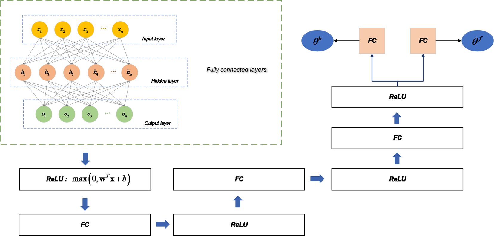
Figure 5 Training process of expansion coefficients in Block.

The expansion coefficients ${\theta }^b$ and ${\theta }^f$ in the previous step are removed from the time series after the transformation of the fully connected neural network when ${\theta }^b=0$ or ${\theta }^f=0$, thus helping the downstream network to perform the prediction task better.

2.4.2 Sequence decomposition

To better interpret the prediction results and reduce the discriminative bias of the model, while facilitating subsequent improvements in the model performance, interpretability is crucial for forecasting models. In time-series forecasting, one of the effective measures to improve the interpretability methods is to decompose the time-series data (Liu et al., 2021). Some of the more common methods for sequence decomposition include additive model decomposition algorithms, X11 decomposition, and STL decomposition (Chen et al., 2020; Gozuyilmaz and Kundakcioglu, 2021).

As shown in Equation (17), the decomposition of sequences is incorporated in the Block of N-Beats network. Block can decompose the time-series data into seasonal and trend simultaneously. In the original N-Beats network, the trend decomposition is processed using polynomials, while the seasonal trend is decomposed using both Fourier functions (i.e., a combined function of sine and cosine waves).

$\begin{array}{ll}{\widehat{y}}_{trend}={\theta }_{}^f{t}^0+{\theta }_{}^f{t}^1+\dots +{\theta }_{}^f{t}^p& (17)\end{array}$

where ${\widehat{y}}_{trend}$ represents the trend vector after time-series decomposition, which consists of a set of polynomials: the expansion coefficients ${\theta }_{}^f$ and time $t^i$ of the fully connected neural network.

The seasonal decomposition then consists of two wave functions, as shown in Equation (18).

$\begin{array}{ll}{\widehat{y}}_{Seasonality}=\sum _{i=0}^{[H/2-1]}{\theta }^f\cos (2\pi it)+{\theta }_{[H/2]}^f\sin (2\pi it)& (18)\end{array}$

where ${\widehat{y}}_{Seasonality}$ represents the seasonal component, and the wave function treats the original sequence as two segments: the first $H/2$ as a cosine wave and the second $H/2$ is decomposed into a sine wave.

The temporal decomposition algorithm of the N-Beats network for interpretable prediction is shown in Figure 6.

Figure 6

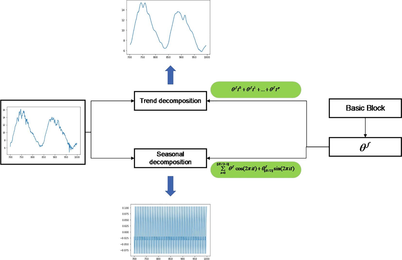
Figure 6 Sequence decomposition algorithm of N-Beats network for model interpretation.

At this point, the training ${\theta }_{}^f$ in the upstream task can make a trend and seasonal decomposition of the interpretability of the prediction results. The prediction sequence in the result needs the forward sequence as input, the forward sequence is decomposed by the same process as above, and the prediction result in the forward sequence can be decomposed by changing the parameter to ${\theta }^b$.

3 Results and discussion

3.1 Data source

The data for this paper were collected at aquaculture sites in Jiangsu, China, and the water quality data were collected from September 2020 until December 2020. The collected water quality information contains six parameters: water temperature, pH, dissolved oxygen, ammonia, nitrogen concentration, conductivity, and water turbidity. The overall data contained 10,625 samples. Some water quality data from September 28, 2020, are shown in Table 1.

Table 1

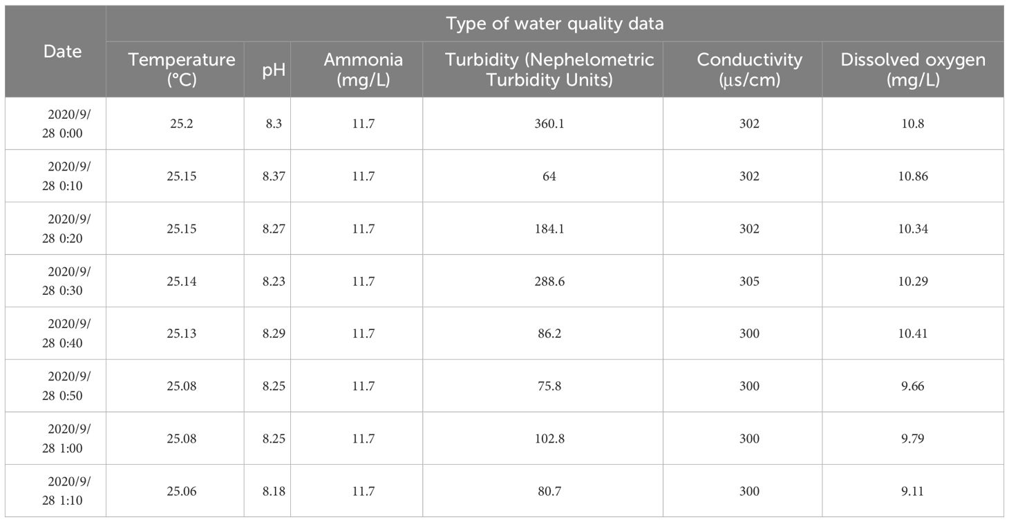
Table 1 Water quality data (partial).

3.2 Model evaluation metrics

Prediction models usually contain multiple evaluation criteria, and this paper used the following evaluation metrics: root mean square error (RMSE), mean absolute error (MAE), and mean absolute percentage error (MAPE).

The formulas for these four evaluation metrics are shown in Equations (19–22).

$\begin{array}{ll}RMSE=\sqrt{\frac{1}{n}{\displaystyle \sum _{i=1}^n}{({\widehat{y}}_i-y_i)}^2}& (19)\end{array}$

$\begin{array}{ll}MAE=\frac{1}{n}\sum _{i=1}^n\left|{\widehat{y}}_i-y_i\right|& (20)\end{array}$

$\begin{array}{ll}MAPE=\frac{1}{n}\sum _{i=1}^n\left|\frac{\stackrel{\wedge }{y_i}-y_i}{y_i}\right|& (21)\end{array}$

$\begin{array}{ll}{R}^2=\frac{{\displaystyle \sum _{i=1}^n}{({\widehat{y}}_i-{\overline{y}}_i)}^2}{{\displaystyle \sum _{i=1}^n}{(y_i-{\overline{y}}_i)}^2}& (22)\end{array}$

Where ${\widehat{y}}_i$ denotes the predicted value of the model for the sample, and $y_i$ represents the true value of the ith sample. n indicates the sample size.

3.3 Noise reduction of water quality data by wavelet transform

Before feeding the time series into the noise reduction network, this paper first used Pearson’s coefficients on the sensor data to see their feature correlation to determine if there was redundancy in the original data. The correlation heat map between the features is shown in Figure 7, and the formula for Pearson’s correlation coefficient is shown in Equation (23).

Figure 7

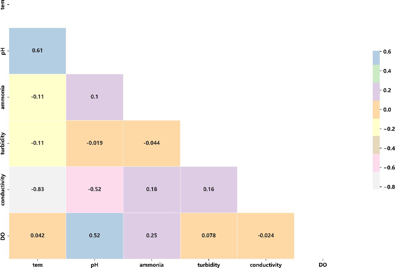
Figure 7 Characteristic correlation between water quality data.

$\begin{array}{ll}\rho (x,y)=\frac{\mathrm{cov}(X,Y)}{{\sigma }_x{\sigma }_y}=\frac{X\ast Y}{\left|X\right|\left|Y\right|}& (23)\end{array}$

where $\mathrm{cov}(X,Y)$ is the covariance between variables, and ${\sigma }_x$ and ${\sigma }_y$ are the standard deviations of variables $X$ and $Y$, respectively.

After the original features were filled by fitting the EM algorithm, this paper used the five-layer wavelet transform for wavelet decomposition of water quality data. Using dissolved oxygen data as an example, the noise threshold for different kinds of water quality information was determined by calculating the confidence interval of the signal. The noise threshold of the wavelet transform was set to 0.3. Figure 8 shows the five components of the dissolved oxygen signal after wavelet decomposition (Coelho and Brito, 2021).

Figure 8

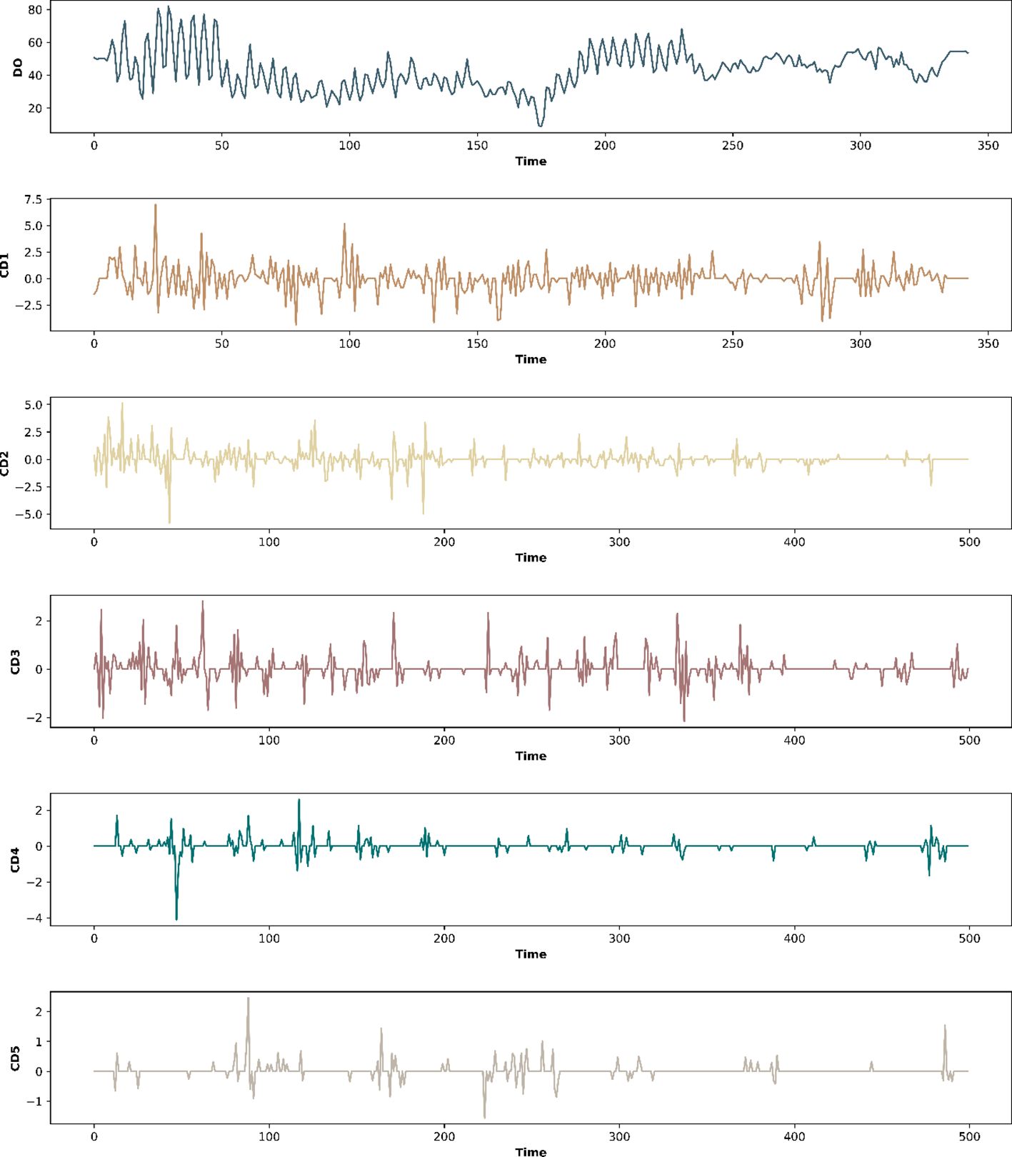
Figure 8 Component signals obtained from dissolved oxygen data after five-layer wavelet decomposition (partial).

After that, this paper used wavelet reconstruction to reconstruct the original signal, and the wavelet transform was performed on six water quality information in the data. The data of the transformed samples are described in Table 2.

Table 2

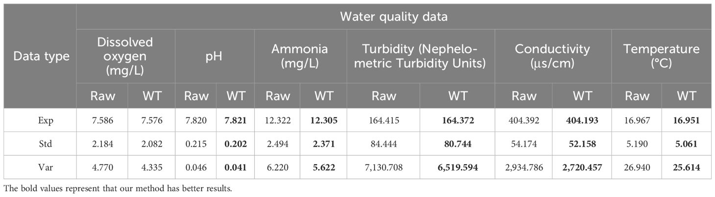
Table 2 Changes in water quality information before and after wavelet transform.

As shown in Table 2, the standard deviations of water quality information such as dissolved oxygen, pH, and ammonia nitrogen concentrations decreased, and after wavelet transform, and compared with the original data, the standard deviations decreased by approximately 4.67%, 6.01%, 4.93%, 4.38%, 3.72%, and 2.49%, respectively. As the overall stability of the sample improves, the accuracy of the model prediction is significantly enhanced. The stability of the sample is crucial for model prediction accuracy, which determines whether the model can maintain consistent performance in the face of different data. When the stability of the samples is improved, the model is better able to learn the intrinsic patterns and features of the data during the training process, thus fitting the data distribution more accurately. This helps to reduce the fluctuations and errors in the prediction results and improve the reliability and stability of the predictions (Kiplangat et al., 2016).

3.4 Dissolved oxygen prediction using GRU–N-Beats network

In this paper, the features of six kinds of water quality information were first extracted because GRU modules can extract water quality features in long series of time dimensions, six groups of GRU modules were designed to extract single water quality variables, and finally the multidimensional water quality data were processed into a single continuous variable as the input of the prediction network through a fully connected neural network. Finally, by feeding these data into the N-Beats network consisting of three consecutive sets of Stacks for double residual learning, the components of the residual learning were summed to obtain the prediction results. In addition, this paper used the Adma optimizer to optimize the training process and the Dropout algorithm to reduce the overfitting phenomenon and improve the model’s generalization ability. Before the model training, the Glorot algorithm was used to initialize the training parameters, and the particle swarm algorithm was used to perform a grid search for the optimal parameters. Finally, 500 epochs were trained on the training set, and the loss curves of training are shown in Figure 9.

Figure 9

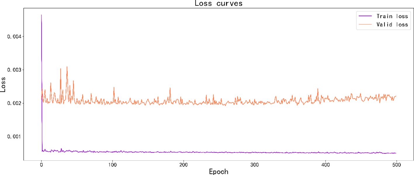
Figure 9 Loss curves on the training and validation sets.

This paper selected 85% of the data for training and validation and the other 15% for prediction. Figure 9 shows the predicted versus actual values of 300 samples. The horizontal axis represents the test samples of dissolved oxygen, and the vertical axis represents the dissolved oxygen content in mg/L. Figure 10 shows the processing results of the dissolved oxygen time series prediction using the proposed method.

Figure 10

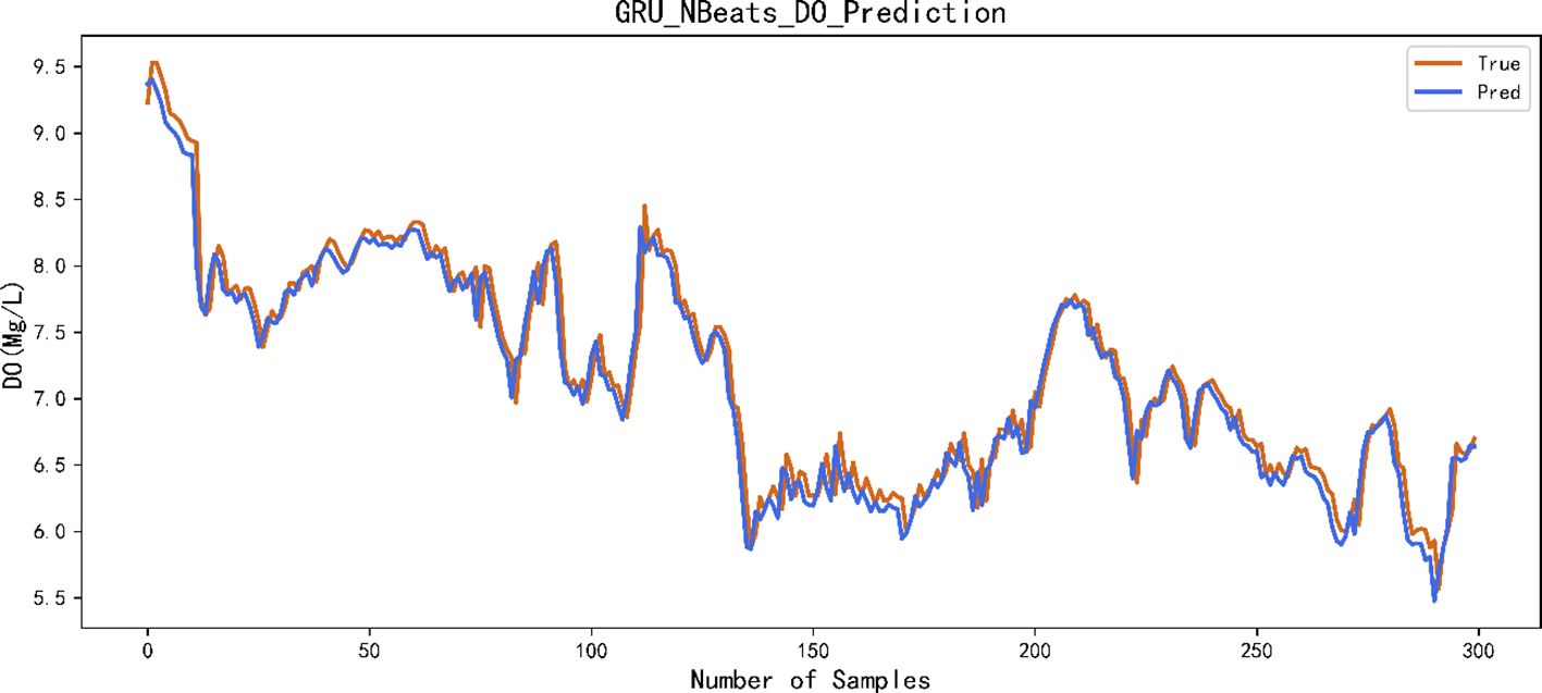
Figure 10 Prediction results of dissolved oxygen using GRU–N-Beats network. GRU, gated recurrent unit.

In addition, the paper compared the forecasting ability of the model over different time spans to ensure that the model can make accurate forecasts over a long length of time period, thus ensuring production safety in the recirculating water culture plant. The prediction results of the model for December 1 and 2, 2020, are illustrated in Figure 11.

Figure 11

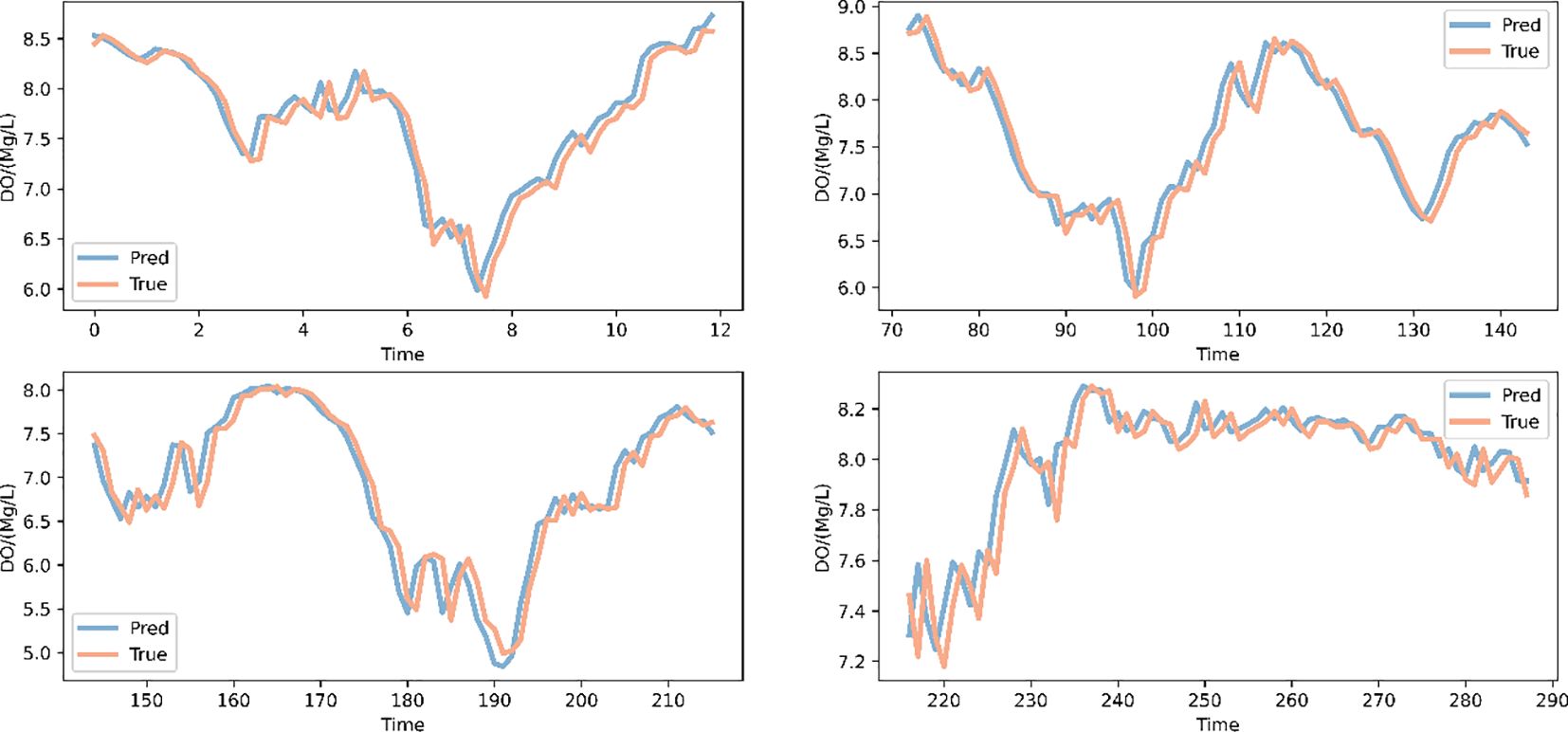
Figure 11 Dissolved oxygen prediction results for December 1–2, 2020.

In addition, in order to enhance the interpretability of the model, this paper decomposed the forecast results into trend and seasonality and rationalized the results in terms of cycles and trends, respectively. First, the prediction results were separated by the remaining modules of Stack in the prediction network and decomposed by polynomial decomposition and triangular wave, and some data of dissolved oxygen prediction were selected for analysis. The results are shown in Figure 12.

Figure 12

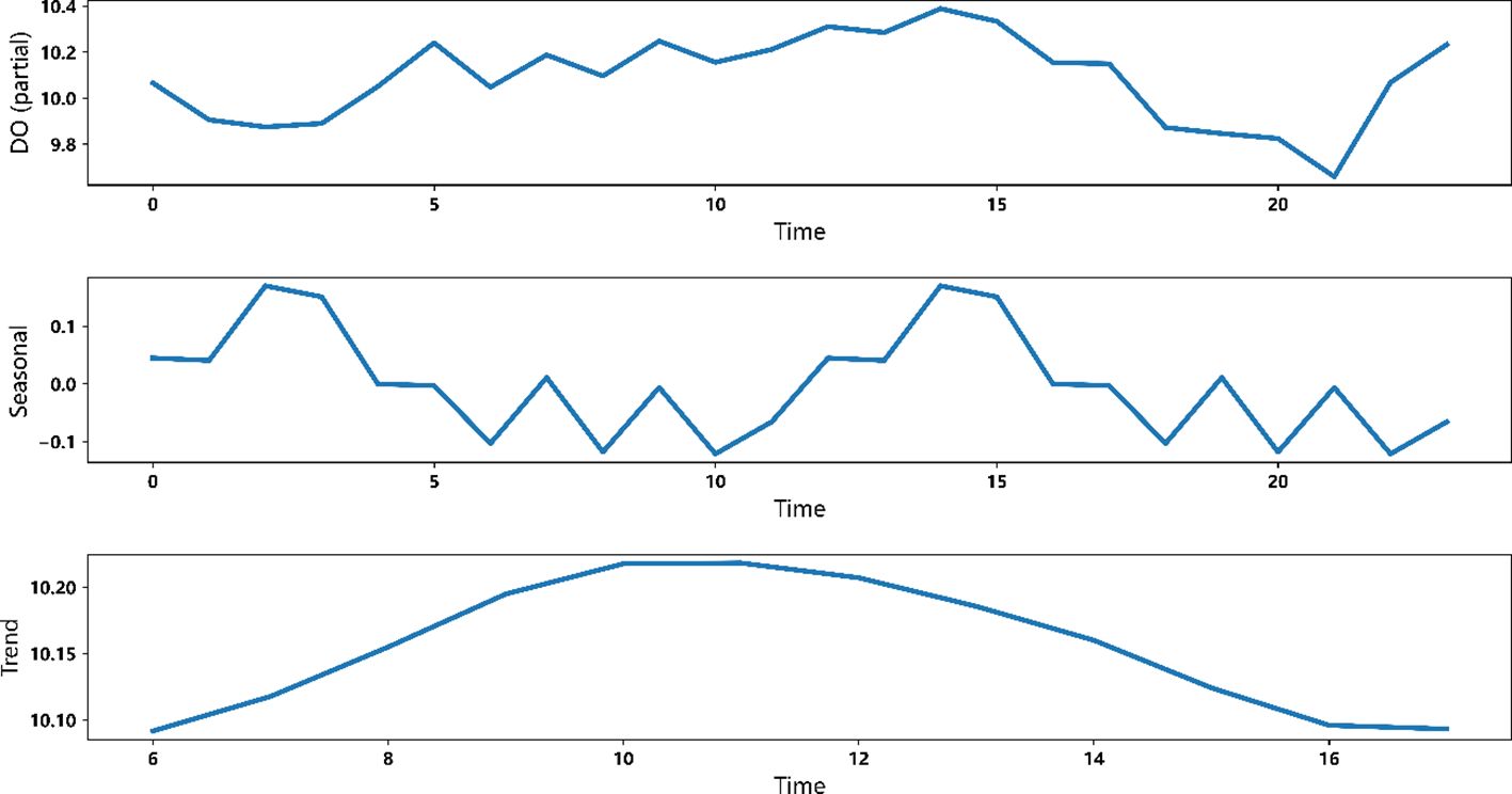
Figure 12 Decomposition of dissolved oxygen prediction results.

3.5 Comparison of the prediction performance with other models

In this paper, four deep learning models, LSTM, TCN, back-propagation neural network (BPNN), and N-Beats, were used to predict the dissolved oxygen concentration, and the results show that the method proposed in this paper has good prediction accuracy. In addition, three evaluation metrics were used, and the results compared with those of other models are shown in Table 3.

Table 3

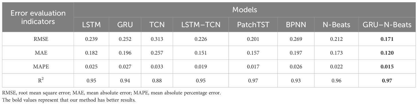
Table 3 Comparison of prediction results of different algorithms on a dissolved oxygen dataset.

According to the results in Table 3, it can be seen that the proposed method has a large improvement compared with other results. Compared with the LSTM model, the proposed method’s RMSE, MAE, and MAPE increased by 28.5%, 34.1%, and 40.0%, respectively. Compared with the GRU model, the proposed method’s RMSE, MAE, and MAPE increased by 32.1%, 38.8%, and 44.4%, respectively. Compared with the TCN model, the proposed algorithm improved the RMSE, MAE, and MAPE by 51.6%, 53.3%, and 54.5%, respectively. Compared with the LSTM–TCN model, the proposed algorithm’s RMSE, MAE, and MAPE increased by 24.3%, 20.5%, and 21.1%, respectively. Compared with the PatchTST neural network, the proposed method’s RMSE, MAE, and MAPE improved by 14.9%, 23.6%, and 11.8% respectively. Compared with the BP neural network, the proposed method’s RMSE, MAE, and MAPE increased by 36.4%, 39.1%, and 42.3% respectively. Compared with the N-Beats algorithm, the proposed method’s RMSE, MAE, and MAPE increased by 19.3%, 30.6%, and 31.8% respectively.

Therefore, the GRU–N-Beats algorithm has better stability in prediction when facing multivariate long-series dissolved oxygen prediction problems. In terms of model applicability, GRU–N-Beats overcomes the problem that N-Beats cannot model multivariate time series at the same time. In addition, it can mine the time-series features of multi-water quality sensor data in the time series and extract and interpret the seasonal and trend elements to obtain better prediction performance.

3.6 Effects of different modules

In order to verify the effectiveness of each module (noise reduction network, feature extraction network, and prediction network) in the whole data processing process, this paper designed the following ablation experiments:

(1) Remove the noise reduction network and use the feature extraction network and prediction network structure to predict the changing trend of dissolved oxygen.

(2) Remove the feature extraction network and use the noise reduction network and prediction network structure to predict the changing trend of dissolved oxygen.

In the ablation experiment, the sample partition structure of the data and the model parameters are consistent. The evaluation results of different network result pairs on RMSE, MAE, MAPE, and R² indicators are shown in Table 4.

Table 4

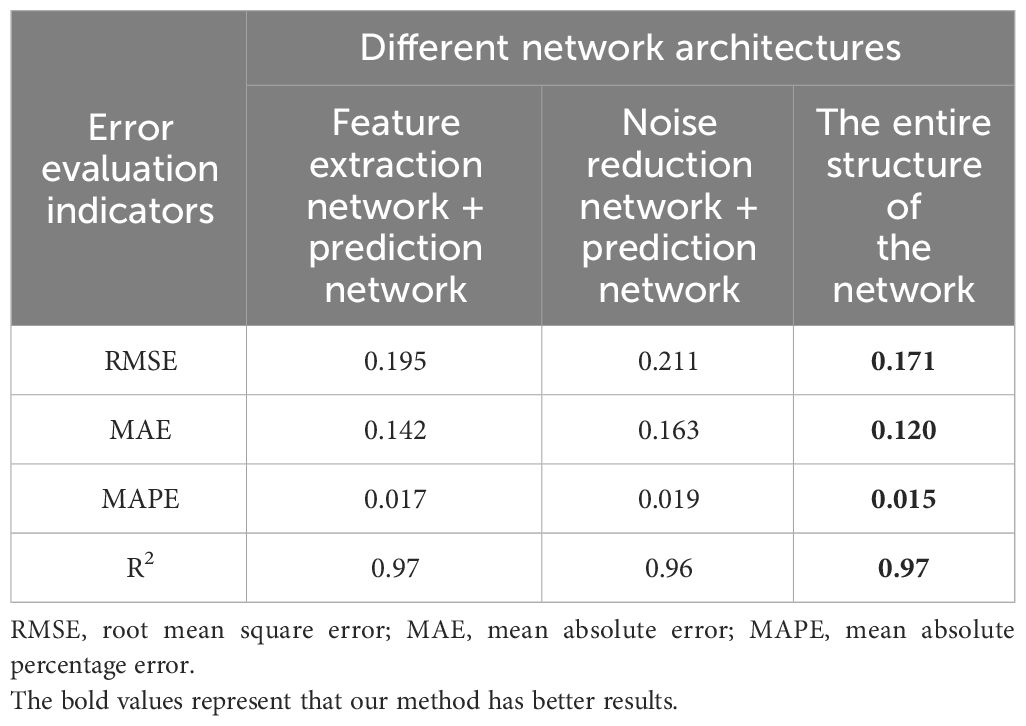
Table 4 Comparison of prediction results of different network structures on the dissolved oxygen dataset.

As shown in Table 4, the network of this paper is compared with the structure without noise reduction network, the complete network structure has the prediction accuracy improved by 12.3%, 15.5%, and 11.8% on the basis of RMSE, MAE and MAPE. Compared with the structure without a feature network, the prediction accuracy improved by 19.0%, 26.4%, and 21.1% based on RMSE, MAE, MAPE, and R².

4 Conclusions

In summary, for the problems of traditional dissolved oxygen prediction such as vulnerability to missing data and complex mechanism of interaction between influencing factors, this paper proposed a dissolved oxygen prediction method based on N-Beats, using the EM algorithm and wavelet transform to preprocess the data, using the gated recurrent unit for feature extraction, and using N-Beats to achieve dissolved oxygen prediction. The experimental results show that the method proposed in this paper has a good prediction effect. First, the water quality data were fed into the noise reduction network, the sample distribution was observed, and outliers were detected and removed. In addition, the maximum expectation algorithm was used to fill the missing data, and the wavelet transform was used to reduce the effect of noise. Then, by building a feature extraction network based on gated recursive units, water quality information was extracted from the temporal and spatial dimensions respectively, and then the features of the six water quality information were fused by a fully connected neural network. Finally, the results were input into the N-Beats network for prediction. The method in this paper overcame the problem of insufficient prediction accuracy due to the inability of the traditional N-Beats network to extract multiple water quality variables simultaneously. Meanwhile, this paper constructed three kinds of Stack for residual learning of water quality information and interpreted the results according to polynomial decomposition and Fourier decomposition. The results show that the algorithm in this paper has better prediction results compared with LSTM, TCN, BPNN, N-Beats, and other algorithms. Therefore, it can satisfy the intelligent prediction of dissolved oxygen in actual production so that control decisions can be made reasonably to ensure production safety and improve farming efficiency in aquaculture.

In future work, more water quality parameters and environmental information can be introduced to improve the prediction accuracy of the model.

Data availability statement

The original contributions presented in the study are included in the article/supplementary material. Further inquiries can be directed to the corresponding author.

Author contributions

ZH: Conceptualization, Data curation, Formal analysis, Funding acquisition, Investigation, Methodology, Project administration, Resources, Software, Supervision, Validation, Visualization, Writing – original draft, Writing – review & editing.

Funding

The author(s) declare that no financial support was received for the research, authorship, and/or publication of this article.

Conflict of interest

The author declares that the research was conducted in the absence of any commercial or financial relationships that could be construed as a potential conflict of interest.

Publisher’s note

All claims expressed in this article are solely those of the authors and do not necessarily represent those of their affiliated organizations, or those of the publisher, the editors and the reviewers. Any product that may be evaluated in this article, or claim that may be made by its manufacturer, is not guaranteed or endorsed by the publisher.

References

Cao X., Liu Y., Wang J., Liu C., Duan Q. (2020). Prediction of dissolved oxygen in pond culture water based on K-means clustering and gated recurrent unit neural network. Aquacultural Eng. 91, 102122. doi: 10.1016/j.aquaeng.2020.102122

CrossRef Full Text | Google Scholar

Cao X., Ren N., Tian G., Fan Y., Duan Q. (2021). A three-dimensional prediction method of dissolved oxygen in pond culture based on Attention-GRU-GBRT. Comput. Electron. Agric. 181, 105955. doi: 10.1016/j.compag.2020.105955

CrossRef Full Text | Google Scholar

Cao S., Zhou L., Zhang Z. (2021). Prediction of dissolved oxygen content in aquaculture based on clustering and improved ELM. IEEE Access 99), 1–1.

Google Scholar

Chen D., Zhang J., Jiang S. (2020). Forecasting the Short-Term Metro Ridership With Seasonal and Trend Decomposition Using Loess and LSTM Neural Networks. IEEE Access 8, 91181–91187. doi: 10.1109/Access.6287639

CrossRef Full Text | Google Scholar

Coelho R. D., Brito N. S. D. (2021). Analysis of RMS measurements based on the wavelet transform. J. Control Automation Electrical Syst. 32, 1588–1602. doi: 10.1007/s40313-021-00770-5

CrossRef Full Text | Google Scholar

Feng R., Jiang W., Yu N., Wu Y., Yan J. (2020). Projected minimal gated recurrent unit for speech recognition. IEEE Access 8, 215192–215201. doi: 10.1109/Access.6287639

CrossRef Full Text | Google Scholar

Gozuyilmaz S., Kundakcioglu O. E. (2021). Mathematical optimization for time series decomposition. OR Spectr. 43 (3), 733–758.

Google Scholar

Hu L., Fan N., Li J., et al. (2021). Dynamic forecasting model for indoor pollutant concentration using recurrent neural network. Indoor Built Environ. 30, 1835–1845. doi: 10.1177/1420326X20974738

CrossRef Full Text | Google Scholar

Huang J., Liu S., Hassan S. G., Xu L. G., Huang C. (2021). A hybrid model for short-term dissolved oxygen content prediction. Comput. Electron. Agric. 186, 106216. doi: 10.1016/j.compag.2021.106216

CrossRef Full Text | Google Scholar

Kiplangat D. C., Asokan K., Kumar K. S. (2016). Improved week-ahead predictions of wind speed using simple linear models with wavelet decomposition. Renewable Energy. doi: 10.1016/j.renene.2016.02.054

CrossRef Full Text | Google Scholar

Kuang L., Shi P., Hua C., Chen B., Zhu H. (2020). An enhanced extreme learning machine for dissolved oxygen prediction in wireless sensor networks. IEEE Access 8, 198730–198739. doi: 10.1109/Access.6287639

CrossRef Full Text | Google Scholar

Li D., Wang X., Sun J., Feng Y. (2021). Radial basis function neural network model for dissolved oxygen concentration prediction based on an enhanced clustering algorithm and adam. IEEE Access 9, 44521–44533. doi: 10.1109/ACCESS.2021.3066499

CrossRef Full Text | Google Scholar

Li W., Wei Y., An D., Jiao Y., Wei Q. (2022). LSTM-TCN: dissolved oxygen prediction in aquaculture, based on combined model of long short-term memory network and temporal convolutional network. Environ. Sci. pollut. Res. 29, 39545–39556. doi: 10.1007/s11356-022-18914-8

CrossRef Full Text | Google Scholar

Liu W., Liu T., Liu Z., Luo H., Pei H. (2023). A novel deep learning ensemble model based on two-stage feature selection and intelligent optimization for water quality prediction. Environ. Res. 224, 115560. doi: 10.1016/j.envres.2023.115560

PubMed Abstract | CrossRef Full Text | Google Scholar

Liu H., Yang R., Duan Z., Ahn J.-H. (2021). A hybrid neural network model for marine dissolved oxygen concentrations time-series forecasting based on multi-factor analysis and a multi-model ensemble - ScienceDirect. Engineering. doi: 10.1016/j.eng.2020.10.023

CrossRef Full Text | Google Scholar

Liu L. C. Y. (2019). Attention-based recurrent neural networks for accurate short-term and long-term dissolved oxygen prediction. Comput. Electron. Agric. 165.

Google Scholar

Kim M. J., Byeon S. J., Kim K. M., Ahn J-H. (2021). Selection of input factors and comparison of machine learning models for prediction of dissolved oxygen in gyeongan stream. J. Korean Soc. Environ. Eng. 43 (3), 206–217. doi: 10.4491/KSEE.2021.43.3.206

CrossRef Full Text | Google Scholar

Ni Q., Cao X., Tan C., Peng W., Kang X. K. (2023). An improved graph convolutional network with feature and temporal attention for multivariate water quality prediction. Environ. Sci. pollut. Res. 30, 11516–11529. doi: 10.1007/s11356-022-22719-0

CrossRef Full Text | Google Scholar

Oreshkin B. N., Carpov D., Chapados N., Bengio Y. (2020). N-BEATS: Neural basis expansion analysis for interpretable time series forecasting. International Conference on Learning Representations.

Google Scholar

Rahman A., Dabrowski J., Mcculloch J. (2020). Dissolved oxygen prediction in prawn ponds from a group of one step predictors. Inf. Process. Agric. 7, 307–317. doi: 10.1016/j.inpa.2019.08.002

CrossRef Full Text | Google Scholar

Ren Q., Wang X., Li W., Wei Y., An D. (2020). Research of dissolved oxygen prediction in recirculating aquaculture systems based on deep belief network. Aquacultural Eng. 90, 102085. doi: 10.1016/j.aquaeng.2020.102085

CrossRef Full Text | Google Scholar

Sang Y. F. (2013). A review on the applications of wavelet transform in hydrology time series analysis (EI). Atmospheric Res. 122, 8–15. doi: 10.1016/j.atmosres.2012.11.003

CrossRef Full Text | Google Scholar

Simone R. (2021). An accelerated EM algorithm for mixture models with uncertainty for rating data. Comput. Stat 36 (1), 691–714.

Google Scholar

Sun J., Li D., Fan D. (2021). A novel dissolved oxygen prediction model based on enhanced semi-naive bayes for ocean ranches in Northeast China. PeerJ Comput. Sci. 7, e591. doi: 10.7717/peerj-cs.591

PubMed Abstract | CrossRef Full Text | Google Scholar

Ta X., Wei Y. (2018). Research on a dissolved oxygen prediction method for recirculating aquaculture systems based on a convolution neural network. Comput. Electron. Agric. 145, 302–310. doi: 10.1016/j.compag.2017.12.037

CrossRef Full Text | Google Scholar

Xiao L., Lu G. (2020). A new refinement of jensen's inequality with applications in information theory. Open Mathematics 18 (1), 1748–1759. doi: 10.1515/math-2020-0123

CrossRef Full Text | Google Scholar

Yang H., Jiang J., Chen G., Mohamed M. S., Lu F. (2021). A recurrent neural network-based method for dynamic load identification of beam structures. Materials 14, 7846. doi: 10.3390/ma14247846

PubMed Abstract | CrossRef Full Text | Google Scholar

Zamani M. G., Nikoo M. R., Jahanshahi S., Barzegar R., Meydani A. (2023). Forecasting water quality variable using deep learning and weighted averaging ensemble models. Environ. Sci. pollut. Res. 30, 124316–124340. doi: 10.1007/s11356-023-30774-4

CrossRef Full Text | Google Scholar

Zhang Y. F., Fitch P., Thorburn P. J. (2020). Predicting the trend of dissolved oxygen based on the kPCA-RNN model. Water 12, 585. doi: 10.3390/w12020585

CrossRef Full Text | Google Scholar

Zhang K., Wu L. (2020). Using fractional order grey seasonal model to predict the dissolved oxygen and pH in Huaihe River. Water Sci. Technol. 83 (2). doi: 10.2166/wst.2020.596

CrossRef Full Text | Google Scholar

Zhao R., Li Y., Sun Y. (2018). Statistical convergence of the em algorithm on gaussian mixture models. doi: 10.48550/arXiv.1810.04090

CrossRef Full Text | Google Scholar

Zhao R., Li Y., Sun Y. (2020). Statistical convergence of the EM algorithm on gaussian mixture models. Electronic J. Stat. 14 (1), 632–660. doi: 10.1214/19-EJS1660

CrossRef Full Text | Google Scholar

Zhou J., Zhu Z. Y., Hu H. T. (2021). Clarifying water column respiration and sedimentary oxygen respiration under oxygen depletion off the changjiang estuary and adjacent east china Sea. Front. Mar. Sci. 7. doi: 10.3389/fmars.2020.623581

CrossRef Full Text | Google Scholar

Zhou X., Wang J., Huang L., Li D., Duan Q. (2022). Modelling and controlling dissolved oxygen in recirculating aquaculture systems based on mechanism analysis and an adaptive PID controller. Comput. Electron. Agric. 192, 106583. doi: 10.1016/j.compag.2021.106583

CrossRef Full Text | Google Scholar