Influence of glacial influx on the hydrodynamics of Admiralty Bay, Antarctica - study based on combined hydrographic measurements and numerical modeling

1 Introduction

Antarctic coastal areas play a crucial role within the broader Southern Ocean system. In the West Antarctic Peninsula (WAP) region more than 650 marine terminating glaciers drain into the ocean, mostly through glacial bays (Cook et al., 2016). Glaciers are significant contributors to global sea level rise due to their high accumulation and ablation rates (Gregory et al., 2013). The glacial water inflow to the ocean influences a wide range of climate-sensitive processes, including shifts in the carbon cycle, ocean acidification, and reorganization of water column stratification (IPCC, 2022). With it, additional carbon, iron, and manganese are transported into the ocean, stimulating phytoplankton blooms and impacting local food chains (Schloss et al., 2012; Forsch et al., 2021). To comprehend the impact of glacial water on the Southern Ocean, it is imperative to understand the hydrodynamics of glacial bays. In particular, it is crucial to understand how bay dynamics respond to variations in the volume of glacial water influx in an era of unavoidable acceleration of the West Antarctic ice sheet melt rates (Naughten et al., 2023). This is because it is expected that unprecedentedly large amounts of freshwater will be introduced into Antarctic coastal waters in the near future, which could have complex and unanticipated consequences for regional hydrodynamics.

Freshwater from glaciers, both from subglacial discharges and submarine melting, mixes with ambient water, forming Glacially Modified Water (GMW; Straneo and Cenedese, 2015). To date, the majority of studies into GMW transport and its influence on coastal hydrodynamics have concentrated on fjords in the northern hemisphere, which differ geomorphologically from Antarctic glacial bays (Cottier et al., 2010). Fjords in Greenland, Alaska, and Spitsbergen are typically long, narrow, and deep. In these basins, described by a large Rossby internal radius (Cottier et al., 2010; Valle-Levinson, 2022), the role of cross-fjord circulation is often minimal, allowing for simplified analysis and modeling in only two dimensions (Motyka et al., 2003; Mortensen et al., 2013; Sciascia et al., 2013).

Motyka et al. (2003) demonstrated that circulation in narrow fjords may be reduced to a single vertical cell with GMW flowing away from the glacial front in the surface layer and ocean waters flowing in towards the front beneath it, upwelling along the glacier, entrained by rising subglacial discharge. This basic model, however, is inadequate in larger Greenlandic fjords, since glacial waters do not always reach the surface due to a larger scale and complex water column stratification (Straneo et al., 2011; Sciascia et al., 2013).

“Unmixing GMW” methods based on hydrographic data are the most widely used techniques for quantifying and tracking pathways of glacial water in the ocean (Jenkins, 1999; Jenkins and Jacobs, 2008; Straneo et al., 2011; Bartholomaus et al., 2013; Mortensen et al., 2013). When GMW spreads in a narrow fjord from a singular glacial front, this analysis can provide almost the entire story of GMW transport since it shows the spatial variability of freshwater content as a function of depth and distance from the outlet. However, in wide bays with complex bathymetry and several marine terminating glaciers, freshwater, after its initial injection, can circulate within the bay, mixing with ambient waters and impacting other ice−water fronts. Three-dimensional (3D) modeling is required to characterize such circulation, and it has been applied successfully in multiple studies. However, the setup used most commonly describes long, deep, and narrow fjords with a single glacial front (e.g., Xu et al., 2012; Sciascia et al., 2013; Cowton et al., 2015; Slater et al., 2018).

Our study area, Admiralty Bay (AB, 62°10′S, 58°25′W), is located in the South Shetland Islands, adjacent to the northern WAP region. AB has the distinctive traits of Antarctic bays rarely seen in the northern hemisphere: it is wide, has a complex coastline, and is adjacent to twenty marine terminating glaciers.

Although previous studies into GMW impact have predominantly focused on the northern hemisphere, recent research has also expanded our understanding of the hydrodynamics of the glacial bays of the WAP. In Marguerite Bay (68°30′S, 68°30′W), seasonal freshwater content variations were measured, and its sources were identified (Clarke et al., 2008; Meredith et al., 2010). The waters of Marguerite Bay and Barilari Bay (65°55′S, 64°43′W) were shown to be subject to intrusions of warm Upper Circumpolar Deep Water (UCDW), which can be an additional driver of glacial melting (Clarke et al., 2008; Cape et al., 2019). The study by Cape et al. (2019) examined the impact of glacial-oceanic interactions on coastal dynamics in Barilari Bay. Specifically, the study concentrated on the formation of surface GMW plumes and its consequences for local biogeochemistry. Lundesgaard et al. (2020) conducted a thorough investigation of the physical properties of water in Andvord Bay (64°50′S, 62°39′W), where the influence of UCDW was found to be limited due to the presence of a sill at the bay’s outlet. Based on these findings, Hahn-Woernle et al. (2020) demonstrated the significant role of surface water thermodynamics in the bay system. Lundesgaard et al. (2019) showed how episodic strong wind events can play a substantial role in the export of GMW from Andvord Bay. Meredith et al. (2018) investigations in Potter Cove (62°14’S, 58°41′W), King George Island (KGI), have revealed the characteristics of glacial meltwater spreading from land-terminating Fourcade Glacier, a glacial form that is more prevalent in the South Shetlands than in the southern WAP region. In conclusion, our knowledge of the Antarctic glacial bay systems has grown over the past few years; a number of hydrodynamical drivers, such as the presence of UCDW, wind, heat content of the upper ocean, and glacial termini type, have been studied. The seasonal variations and long-term increase in glacial runoff have been shown through the analysis of hydrographic and glaciological data (Meredith and King, 2005; Vaughan, 2006; Clarke et al., 2008). However, the impact of glacial influx on the hydrodynamics of Antarctic glacial bays, particularly how it affects water level oscillations, circulation patterns, water column stratification, and freshwater distribution, have not yet been thoroughly studied in this region. Moreover, there have not been many prior attempts to analyze the seasonal variations in these processes. This is the goal of this study.

The structure of this paper follows the logical reasoning underlying this project, in which numerical modeling is based on the conclusions from the analysis of observational data. The study area is described in Section 3.1, followed by the details of in situ measurement methodology (Section 3.2.1). Section 3.2.2 provides a general overview of water property variations in AB. A 3D circulation model was developed based on the conclusions of Section 3.2.2 (technical details in Section 3.3.1). The problem of determining the appropriate location of glacial water injection points in the model was essential. Therefore, the Section 3.3.2 describes its theoretical background and presents the results of model test runs conducted to examine it. The model was run in fourteen scenarios with an increasing glacial influx volume. The findings revealed the character and magnitude of glacial water’s impact on water level variations, circulation, freshwater thickness (FWT), and pycnocline depth in the bay (Section 4.1). This enabled identification of boundaries between regions dominated by glacially and tidally-driven circulation patterns (Spall et al., 2017). Finally, in Section 4.2, an attempt was made to estimate the glacial runoff volume into AB. This estimate was based on a novel approach in which differences between modeling results and in situ measurements were used to select an optimal (most probable) influx volume at a given time instance, yielding a 136-record-long timeseries of glacial influx volumes in the period from December 2018 to February 2023 (Mortensen et al., 2014; Straneo et al., 2011; Sciascia et al., 2013). The results are followed by a discussion in Section 5.

The overall objective of this research is to identify key features of Antarctic bay’s hydrodynamics, and its variability in response to glacial influx. It is one of the first attempts to model a 3D circulation within a bay with multiple marine-terminating glaciers, showing relative significance of different forcing mechanisms. Additionally, by comparing measurement and model results, seasonal estimates of glacial influx volumes were obtained.

2 Materials and methods

2.1 Study area

Admiralty Bay is a large inlet of KGI, the biggest island in the South Shetlands (Figure 1), a region described as especially sensitive to climate change (Bers et al., 2013). The acceleration of glacial melting during summer (Rückamp et al., 2010) and the recent absence of sea ice during winter are the most prominent indicators of this vulnerability (Eayrs et al., 2021; National Snow and Ice Data Center, C, 2023).

Figure 1

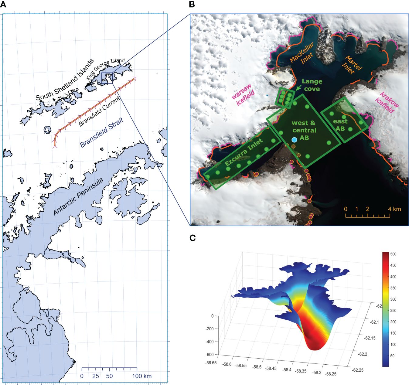
Figure 1 Admiralty Bay. (A) Regional map (Gerrish et al., 2021), Bransfield Current as per Thompson et al. (2009); (B) Admiralty Bay map; ocean-ice boundaries: in 2021 marked with pink lines (Gerrish et al., 2021), and in 1990 – orange lines (Battke, 1990); red points correspond to known creek outlets (Potapowicz et al., 2020 and observations); green points show in situ measurement sites and green boxes their groupings; blue dot indicates wavemeter mooring location (inset based on Sentinel imagery, 29.12.2021); (C) AB bathymetric map (m) and modeling domain.

KGI is covered in 90% with ice, divided into interconnected icecaps (Simões et al., 1999). Twenty-five percent of AB’s 150 km long coastline consists of ice−water boundaries, formed by twenty maritime glaciers draining directly into the bay waters (indicated with orange lines in Figure 1A). All of them are relatively shallow (Figure 1C), with an estimated maximum grounding depth of ~150 m, and the majority of glacial fronts submerged by less than 50 m. Because of that, AB glacial fronts are considered to be nearly uniform vertically, without evidence for undercutting or floating tongues (Carroll et al., 2016). AB glaciers can be classified as intermediate forms between polar and temperate glaciers, with both geothermal and frictional heating as well as external warming inducing water discharge into the ocean (Jenkins, 2011). A comparison of a regional map from 1990 and recent satellite imagery (Battke, 1990) shows a significant retreat of local glacier fronts over the past 31 years (Figure 1B, orange lines – ice-water boundaries in 1990, pink lines – ice water boundaries in 2021).

Additional freshwater input into the bay is produced by glacial creeks, which frequently carry waters from glaciers that have recently retreated to land. Their existence and the amount of water being supplied through them vary significantly throughout the year. Consistently reoccurring summer creeks (17 separate outlets) noted by Potapowicz et al. (2020) and observed by the crew of the Arctowski Polish Antarctic Station have been marked in Figure 1B with red points. The mean annual precipitation in AB is approximatively 0.07 Gt (Plenzler et al., 2019). Considering estimated annual mean value of glacial influx of 0.434-0.632 GT (see sections 4.2 for details) the input from precipitation to the AB freshwater budget is relatively minor and was not considered in this analysis.

AB has an area of 150 km² and has been previously described as a wide fjord, however, geomorphologically, it is a tectonic estuary (Valle-Levinson, 2010), formed by geological faults (Majdański et al., 2008), which explains its distinction from northern hemisphere fjords. For the purposes of this study, a new, hitherto most precise bathymetric map of AB has been created, compiling data from Battke (1990), Majdański et al. (2008); Magrani et al. (2016) and self-conducted ADCP measurements (Figure 1C). It shows that AB’s mean depth is 160 m, but in its central part there is a relatively narrow trough up to 600 m deep. AB is connected with Bransfield Strait through a 8 km wide opening, notably, without a well-defined sill.

Tidally controlled water level shifts oscillate between −1.5 and 1 m at the AB outlet (Padman et al., 2002). Locally, the most common wind direction is SW, present for around 25% of the time; wind events from other directions take up from 5 to 10% of the time (Plenzler et al., 2019). The occurrence frequency of long-lasting periods of along-fjord (NW or SE) katabatic winds, controlling water exchange with the ocean is, low. This is in contrast to Greenland, as noted by (Spall et al., 2017). Nevertheless episodic occurrence of this process is possible as recorded, e.g., in Andvord Bay by Lundesgaard et al. (2019).

In Bransfield Strait, Bransfield Current flows in a northeastern direction along the southern border of the South Shetlands and creates an effective barrier from outside currents (Zhou et al., 2006; Poulin et al., 2014; Moffat and Meredith, 2018); see Figure 1B). This blocking mechanism is strengthened by local bathymetry, which, close to the AB outlet, drops rapidly to over 2000 m, so that relatively shallow AB-shelf waters are only to a limited extent influenced by deep ocean hydrodynamics. Consequently, currents impacting the AB directly are forced by tides, with the Coriolis force playing a key role, which together drive water exchange with the ocean. According to Zhou et al. (2020) the full water exchange between AB and Bransfield Strait takes approximately 147 hours.

2.2 Hydrographic measurements

2.2.1 Methodology

Since December 2019, a comprehensive in situ measuring campaign has been conducted using YSI Exo CTD+ sondes to investigate the AB water properties. It comprised of vertical measurements of water conductivity, temperature, pH, turbidity, and dissolved oxygen, dissolved organic matter, chlorophyll A, and phycoerythrin content at 31 sites across four years. The openly accessible data up until January 2022 can be found in the PANGAEA repository (Osińska et al., 2022). Detailed information regarding the scope and methodology of data collection is described in Osińska et al. (2023). Measurements conducted using an unaltered methodology have continued up until February 2023, and their findings have been analyzed in this study. For the present analysis, 23 measurement sites with depths exceeding 10 m were chosen (Figure 1A; green points) and divided into four zones (Figure 1A; green boxes):

• west and central AB – west and central region of AB’s main body,

• east AB – sites in the east part within the main body of AB,

• Ezcurra Inlet – within the smaller western inlet of AB,

• Lange cove – sites less than 1 km away from the medium-sized Lange glacier

Measurements with missing salinity records and those from the depths above 0.5 m have been excluded from the analysis (due to high uncertainty of near-surface measurements It was found that several salinity records had abnormally high mean values of >35.5, which raised suspicions. Consequently, it was decided that extracting outliers from the dataset was appropriate. A time-averaged salinity profile [ $S^x(z)]$ was calculated for each site from all measurements at that site $s_n^x(z)$, where z denotes depth, x denotes a specific site and n is an index of individual measurement at that site. The following records have been classified as outliers and removed from the dataset:

• 5% of profiles at each site with the largest standard deviation of differences $({\sigma }_D)$ from that site’s mean salinity profile

• 5% of profiles at each site with the largest difference between vertically-averaged $s_n^x(z)$ and vertically-averaged $S^x(z)$

After this procedure, the remaining dataset consisted of 1830 profiles from 136 days and all seasons of the year.

Freshwater thickness (FWT) was determined for all profiles using the Holfort et al. (2008) formula:

$\begin{array}{ll}FWT={\int }^{}\left(\frac{S_{ref}-s_n^x(z)}{S_{ref}}\right)dz& (1)\end{array}$

where S_ref is a reference salinity value. S_ref was determined for each measurement day as the mean salinity value from all measurements from that day below 60 m. The decision to use records from below 60 m was based on modeling results that showed glacial water spreading maximally to this depth (details in Section 4.1.2).

2.2.2 Results analysis

Figure 2 provides a comprehensive depiction of the fluctuations in AB water properties over four years of hydrographic measurements (see also this data presented in vertical profiles of salinity in Supplementary Figure 1). Overall, the water temperature varied in a range of −2 to 2°C, while the salinity ranged from 33.3 to 34.6 (Figures 2A–H).

Figure 2

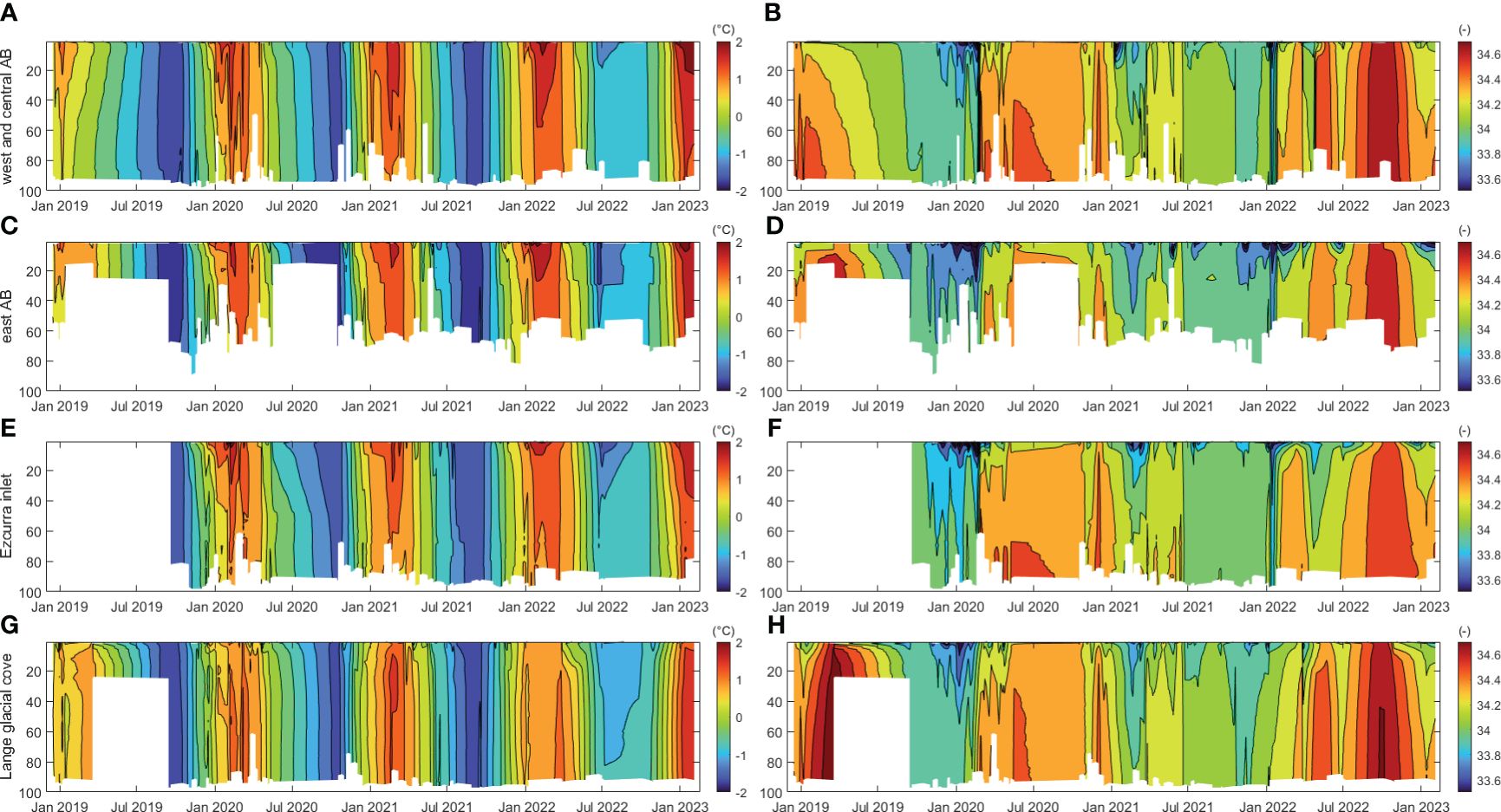
Figure 2 Overview of salinity and temperature records in AB. (A, C, E, G) mean temperature (°C) and (B, D, F, H) mean salinity in four zones: (A, B) – west and central AB, (C, D) east AB, (E, F) Ezcurra inlet, (G, H) Lange cove.

The surface freezing line seen in TS diagrams (Figure 3) shows that most of the time AB water properties were well above freezing conditions during all seasons of the year (details in Osińska et al., 2022). This is the reason for the absence of winter sea ice coverage in AB over the course of the measuring campaign.

Figure 3

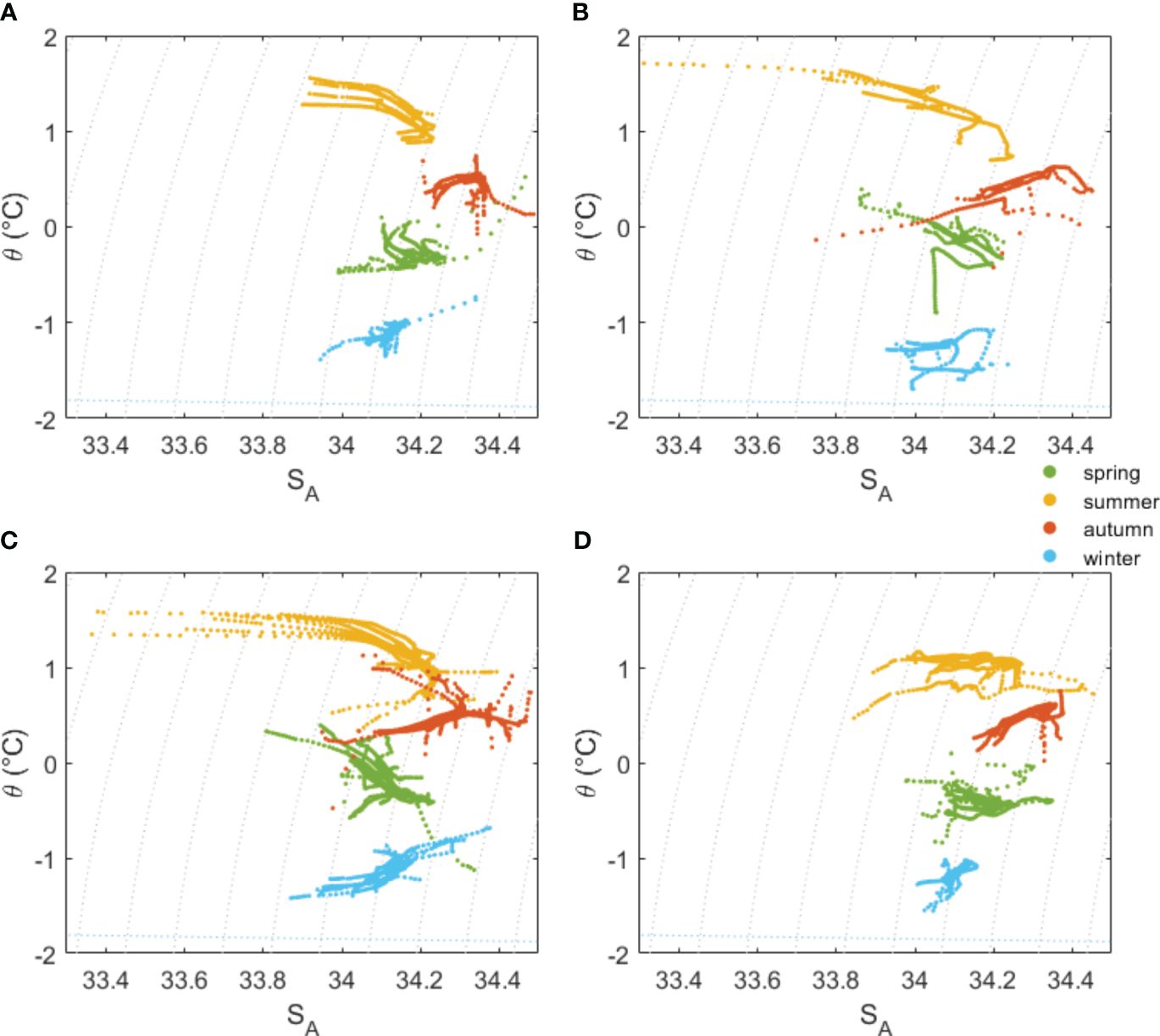
Figure 3 TS diagrams of mean seasonal values from each site; (A) – west and central AB, (B) east AB, (C) Ezcurra inlet, (D) Lange cove; blue dotted line – surface freezing line.

The freshening of AB’s surface water during austral summer (Figures 2B, D, F, H) and the corresponding peaks in FWT (Figure 4) indicate the presence of GMW. This is because marine terminating glaciers are a primary source of freshwater in the northern WAP region, as established by Powell and Domack (2002). Additionally, it has been determined that the contribution of sea ice and precipitation to AB’s freshwater content is limited. No evidence of fresher water plumes in subsurface layers was detected (Figure 2H and more details in Osińska et al., 2023). Hence, the GMW continuously exhibits the highest buoyancy among the water masses in the AB region, a finding that has been corroborated by prior investigations conducted in the area (Monien et al., 2017; Meredith et al., 2018; Osińska et al., 2021).

Figure 4

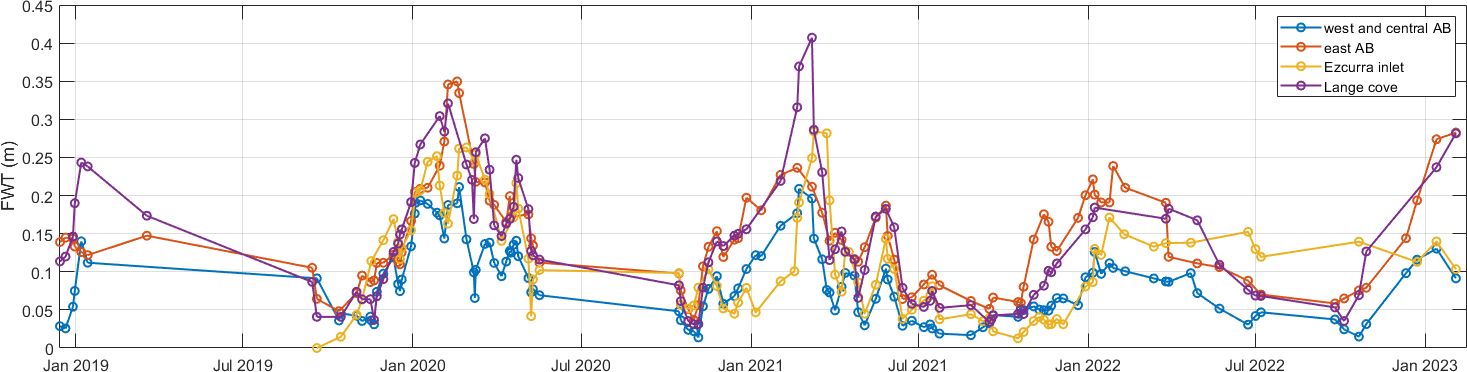
Figure 4 Mean freshwater thickness (m) from all sites in four zones in AB.

The FWT variations exhibit a similar seasonal pattern across the entire AB. However, FWT values are lowest in the west and central AB, with a mean of 0.09 m and a median of 0.07 m (Figure 4). The FWT mean and median values in the east AB are 0.15 m and 0.14 m, respectively; in Ezcurra Inlet, they are 0.12 m and 0.10 m; and in Lange cove, they are 0.14 m and 0.12 m. This would suggest that the presence of GMW is lowest in the western regions of the main basin of AB and noticeably highest in its eastern region, even surpassing that of regions directly adjacent to glacial fronts, such as sites in the Lange cove.

TS diagrams, as shown in Figure 3, are used to differentiate between water masses inside of the AB. AB waters during the winter are generally homogenous, with temperature and salinity marginally rising as depth increases. During the spring season, a fresher and warmer layer of water is formed on the surface, overlaying waters characterized by increasing salinity and temperature with depth. Two layers in the AB water column are also present during summer and autumn. The summer surface layer experiences maximum freshening (average salinity dropping to 33.2) and warming (mean temperature ranging from 1 to 1.5°C). During the autumn, the upper layer, in comparison to the summer season, exhibits lower temperatures and higher salinity.

Observations indicate that AB contains up to two characteristic water layers throughout the course of a year. The distribution of these layers’ salinity and temperature values can be largely attributed to atmospheric and glacial influences. The water mass found below the surface layer during the seasons of spring, summer, and autumn, as well as the principal water mass observed during winter, shall be referred to as ambient water (AW). This water mass is primarily impacted by the waters of the Bransfield Strait and by atmospheric forcing. AW exhibit relatively small variability throughout the year and display typical patterns of seasonal fluctuation commonly observed in estuarian deep waters (Cottier et al., 2010). Fresh surface waters found in spring, autumn, and particularly during the summer are classified as GMW. GMW consists of a mixture of AW and glacial water that originates from subglacial discharge, submarine melting, glacial creeks, and icebergs. These waters are heated and cooled to varying extents through atmospheric forcing. The lowest summer surface temperatures were recorded in Langel cove since the freshly formed GMW surface layer has a limited duration of atmospheric exposure. Notably, there is a possibility of external freshwater entering AB at the surface, which may be indistinguishable from GMW using solely salinity records.

The presence of warm and highly saline Atlantic Waters in Greenland (Straneo et al., 2011; Sciascia et al., 2013; Slater et al., 2018) and CDW in the Antarctic (Moffat et al., 2009; Cape et al., 2019) has been shown to directly stimulate glacial melting and play an important role in shaping the hydrodynamics of glacial bays. The hydrographic data analyzed here does not support the existence of such warm external water masses in AB. The measurements conducted in this investigation were limited to a maximum depth of 100 m. Consequently, it is possible that distinct water masses could infiltrate deeper AB waters and remain undetected. Nevertheless, the probability of such an event and its substantial influence on AB’s glacial-oceanic boundary is low. Because water depth near AB glaciers seldom exceeds 100 m (Figure 1C), any warmer and more saline water intrusions would be unable to reach glacial fronts unless their presence were recorded at shallower measurement sites. Additionally, earlier measurements conducted in AB over a wider vertical range also did not find any signs of the presence of such water masses (Carbotte et al., 2007). Finally, studies of regional ocean circulation concluded that CDW intrusions into AB are unlikely (Hofmann et al., 2011; Sangrà et al., 2011).

The general two-layered stratification enables the determination of the internal Rossby radius $(r_i=\frac{c_i}{f}$, where ${c_i}^2$ is the internal wave speed and f is the Coriolis parameter) which serves as a metric for evaluating the relative significance of water column stratification in comparison to rotation (Cottier et al., 2010). In the AB, depending on conditions, the internal Rossby radius varies between 0.41 and 11.86 km (its average values are 0.91 in winter, 1.00 in spring, 1.39 in autumn and 1.83 km in summer). Therefore compared to the ~8 km wide opening, it indicates that the AB can be classified as a “broad bay”, where the presence of cross-bay circulation has substantial importance. This is valid for all seasons, even the period of enhanced glacial melting, when freshwater influx strengthens the water column’s stratification.

2.3 Hydrodynamic modelling

2.3.1 Model setup

The presence of a two-layered stratification in AB, where the surface layer consists of the most buoyant layer of glacial meltwater (GMW), is reminiscent of the conditions outlined in the small-fjord single-cell circulation model proposed by (Motyka et al., 2003). However, due to the “broad” character of the bay, the AB model must be three-dimensional.

Modelling of AB hydrodynamics has been performed using the open-source Delft3D-Flow model, developed as part of a Delft3D suite created specifically for coastal, river, and estuarine hydrodynamics (Deltares, 2020). The calculations were performed on a high-resolution curvilinear grid of over 30,000 points, thus, an average grid cell corresponds to an area of approximately 55 m². Figure 1C shows the entire model domain. The analysis was conducted in 3D, with fifty layers utilizing a vertically scaled σ-coordinate system, with more densely spaced layers toward the domain’s bottom and top. The bathymetric map shown in Figure 1C was used with a single smooth, ~10 km long open boundary between AB and Bransfield Strait.

The model was driven by tides, and temperature and salinity gradients. The tidal water level at the open boundary was calculated using the CATS2008 Antarctic tides model (Padman et al., 2002). Temperature and salinity data reanalysis by Dotto et al. (2021) was used to determine temperature and salinity values at the open boundary since it is the most robust data source for water properties in the northern WAP region, combining the majority of available in situ measurement records from 1990 to 2019. Seasonally averaged (for spring and summer) reanalysis values were extracted from a grid point closest to the model’s open boundary and interpolated in time and space to create varied vertical salinity and temperature profiles. Dotto et al. (2021) results show that Bransfield waters are weakly stratified (Supplementary Figure 2) with seasonal mean temperature and salinity variations of -1.23–0.51°C and 34.22 –34.27. The in situ measurement results from Osińska et al. (2023) were used to determine initial values of water salinity and temperature inside AB, which were uniformly set throughout the domain. It has been found during preliminary model testing that after less than three days of simulations, the salinity stratification in the whole bay was predominantly influenced by the open boundary input, therefore no variation in the initial conditions setting was necessary.

To capture the variability associated with the entire range of tidal patterns in this region, calculations lasted 58 days (from 1.12.2021 to 28.01.2022), consisting of 3.5 days of model warm-up followed by two full lunar cycles.

Following Deltares recommendation, bottom roughness was calculated using the 3D Chézy formula (Deltares, 2020), and assumed spatially homogenous due to lack of information on bottom roughness variations in AB. During model testing, it was discovered that unreasonably high values of kinetic energy dissipation rate (>1000 m²/s³) were obtained close to the open boundary after approximately two days of calculations and persisted throughout the simulation length. It was determined that this was caused by inappropriately assessed bottom roughness. Through several additional test runs it was experimentally found that uniform 3D Chézy bottom roughness coefficients of 40 m^1/2/s, in both U and V directions, is the highest coefficient value which does not result in unrealistic energy dissipation anomalies, which cause a rapid increase in flow velocities near the open boundary, and consequent model destabilization. The energy dissipation rates had a reasonable median value in the order of 10^-8 m²/s³ (comparable values were found in Andvord Bay by Lundesgaard et al., 2020). Although they were greater in the bottom layer they were still within the realistic range of 10^-6 -10^-4 m²/s³ (see Supplementary Table 1, Inall and Rippeth, 2002). Therefore, it was determined that a bottom roughness coefficient of 40 m^1/2/s was suitable and used all subsequent calculations.

Test runs were carried out to investigate the impact of boundary conditions on the model domain. In general, its impact was not significant. The only part of the model domain where the results were affected by the boundary conditions is the outermost, inflow region in the west (see Section 4.1.2). This implies that the results in this area should be interpreted with caution. The Reynolds number, which is a measure of turbulence, was in the range of 10⁴–10⁶ close to the open boundary and was lower than 100 close to the inner inlet heads.

Additional information regarding the model configuration can be found in Supplementary Table 2. Importantly, as indicated by the aforementioned description of the model configuration, no atmospheric forcing was considered, i.e., ocean-atmosphere momentum, heat, and moisture fluxes were set to zero. This decision is justified by the fact that, first, the salinity differences between the oceanic and glacial waters dominate the density structure and gradients in the domain of study, and second, volume fluxes associated with tidal currents dominate those generated by wind, particularly over the time scales of several tidal cycles considered here. Such simplification is not unusual in studies at this scale (Straneo et al., 2011).

The typical density anomaly of water entering through the open boundary and that of the meltwater is σ=27.4 kg/m³ (at S=34.1 and T=−0.2°C) and σ=0 kg/m³ (at S=0 and T=0°C), respectively. The highest recorded value of surface water temperature observed in AB in the summer was 3.54°C (at 1.15 m depth), which was exceptionally high (Osińska et al., 2023); the corresponding density anomaly at S=32.56 is σ=26.0 kg/m³. Therefore, the contribution of temperature to the net variability of water density in AB is minor. Accordingly, the core of the analysis and discussion in the following sections is considering factors driven by salinity fluctuations. Since seasonal salinity variations derived from Dotto et al. (2021) dataset are small (<0.1 difference between mean seasonal values) model setup accurately replicates AB open boundary conditions throughout the year.

For model validation purposes, an RBR wavemeter was moored within Admiralty Bay (location indicated with blue dot in Figure 1A) logging water level at 2 Hz frequency during the period from 6.12.2021 to 21.12.2021. The standard deviation of differences between Delft3D model data at this location and in situ RBR measurements is 0.08 m, the bias is 0.03 m, and their correlation coefficient is 0.99, i.e., the modeling results correspond very closely to the real water level changes in that part of AB. Analogously, CATS2008 compared with RBR measurements has a 0.08 m standard deviation of differences, a bias of 0.01 m, and correlation coefficient of 0.99.

2.3.2 Location, dispersal and volume of glacial freshwater influx

The representation of interactions between glaciers and oceans is a crucial component in establishing the framework for glacial bay hydrodynamical modelling. The description of oceanic dynamics near marine terminating glaciers often relies on the buoyant plume theory (BPT). The BPT explains how freshwater discharged from underneath the glacier upwells along the glacial front, entraining and mixing with ambient waters to form a GMW plume. This plume then induces the submarine melting of the glacier’s front (Jenkins, 2011). The submarine melt rate is influenced by subglacial discharge volume and ambient water temperature; however, this relationship varies depending on the study location (Kimura et al., 2014; Xu et al., 2012; Sciascia et al., 2013). When GMW reaches its depth of neutral buoyancy, which may occur at or below the ocean surface, it forms a layer of distinct properties within the water column (Jenkins, 2011). The influence of glacial water on ocean hydrodynamics is contingent upon the distribution of subglacial discharge points, namely whether they are channelized or uniformly distributed along the glacial front, and the momentum of the discharge (Cowton et al., 2015; Slater et al., 2018).

The Buoyant Plume Model (BPM) coupled with the general circulation model (GCM) is currently considered the most sophisticated method for investigating the hydrodynamics of glacial bays (Cowton et al., 2015). However, its application may not always be necessary or practical. In an earlier investigation conducted by Chauché et al. (2014) observational data indicated that subsequent to channelized release, subglacial influx rapidly spreads laterally along the glacial front, effectively blurring the distinction between effects of localized and uniformly dispersed freshwater injection points. The study by Sciascia et al. (2013) demonstrated that the hydrodynamics of near-glacial waters is influenced to a greater extent by the volume of subglacial discharge than the momentum of its inflow. The usage of the BPM coupled with GCM for the purpose of modeling the hydrodynamics of bays with multiple ice-water boundaries is challenging. Firstly, such multiway coupling is computationally expensive. Furthermore, it requires detailed bathymetric and glaciological data, including discharge location points, volumes, and submarine melt rates (Carroll et al., 2016) which is currently unattainable in AB and, we argue, in the majority of glacial bays in Antarctica.

In light of the practical challenges involved, a question arises regarding the extent to which accurately reproduced vertical location and velocity of glacial water influx is significant for the understanding of general AB hydrodynamics. In order to address this question, several iterations of model tests were conducted, in which glacial water discharge locations and velocities were varied. The following are the identifiers and details of these test runs:

• H0 - test run with glacial water discharged from all glaciers, homogenously through the entirety of glacial front, with zero initial velocity (treated as reference case for other scenarios)

• H2 - test run with glacial water discharged from all glaciers, homogenously through the entirety of glacial front, with an initial velocity of 2 m/s

• S0 - test run with glacial water discharged from all glaciers subglacially, with zero initial velocity

• S2 - test run with glacial water discharged from all glaciers subglacially, with an initial velocity of 2 m/s

In order to emphasize the potential influence of glacial discharge velocity on AB hydrodynamics, a high value of 2 m/s was selected for testing (Xu et al., 2012; Cowton et al., 2015). The volume of the glacial discharge for all test runs was established at ~6 m³/s per 1 km of glacial front, a value that was deemed reasonable for the AB region during the summer melt season (see section 4.2).

Three measures were employed to examine disparities between test run results: FWT (Figures 5A–D), pycnocline depth (Figures 5E–H), and depth-averaged flow velocity (Figures 5I–L). These metrics serve as the foundation for further analysis of AB hydrodynamics, making them suitable instruments for determining if the results of test scenarios exhibit substantial differences between each other. FWT was calculated using Formula (1), where S_ref was determined as the mean salinity from below 60 m across the entire AB. Given the stratification of model open boundary waters, the utilization of this FWT calculation method shows the presence of freshwater influx from the Bransfield Strait into AB. Hence, in order to illustrate the distribution of freshwater originating exclusively from AB glaciers, the FWT values calculated for a scenario devoid of glacial water inflow (scenario 0 m³/s) were subtracted from the FWT results of the four test runs. The pycnocline depth was calculated as the depth at which dσ/dz< 0.025 kg/m³. The data that have been analyzed and presented in Figure 5 were averaged over a period from January 1st, 2022 to January 28th, 2022, which corresponds to a one complete lunar cycle.

Figure 5

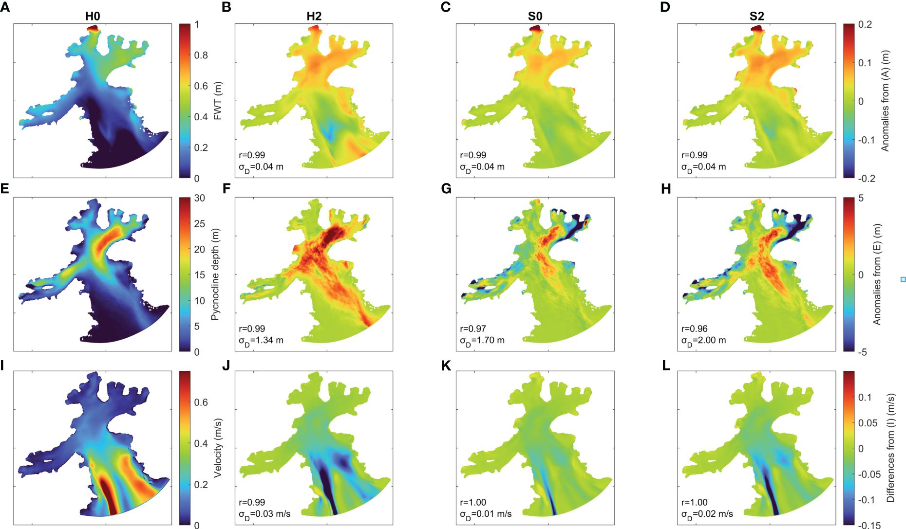
Figure 5 Comparison between model results with different glacial discharge locations and velocities. (A–D) FWT (m); (E–H) Pycnocline depth (m); (I–L) depth averaged velocities in m/s; (A, E, I) H0 scenario – reference case; (B, F, J) H2 scenario differences from the reference case; (C, G, K) S0 scenario differences from the reference case; (D, H, L) S2 scenario differences from the reference case. r, ${\sigma }_D$– correlation coefficients and standard deviation of differences between shown results and reference case respectively. All figures depict mean values from period from 1.01.2022 to 28.01.2022.

All test run results show consistent patterns in the FWT, pycnocline depth, and flow velocity values distributions across the AB Supplementary Figure 3). On the other hand, discrepancies are visible when comparing maps of differences between test runs and the reference case (H0) results (Figure 5).

For all test scenarios the FWT values are highest in the northwest region of AB, ranging from 0.35 to 0.55 m, (Figures 5A–D). In that area the three scenarios H2, S0, and S2 have slightly greater FWT values (<0.1 m) than the reference scenario H0. The overall FWT differences between scenarios range from −0.1 to 0.15 m (Figures 5B–D). In test runs with solely subglacial discharge, narrow regions of elevated FWT form along glacial fronts. The biggest differences in FWT and pycnocline depth are observed in scenario H2 (Figures 5B, F). For instance, in an area of a maximum pycnocline depth (~25 m) for H0, the pycnocline depth increases by up to 4 m in S0 and S2, and by over 6 m in H2. In S0 and S2 scenarios the presence of subglacial discharge and subsequent turbulent mixing prevents pycnocline formation in regions close to glacial fronts (blue areas in Figures 5G, H). Crucially, the overall flow pattern remains consistent in all examined cases, characterized by a strong influx from Bransfield Strait along the AB’s western bank and an outflow in the east (see more details in section 4.1.2). The differences in flow velocities, shown in Figures 5I–L, are largest close to the AB opening. In scenarios H2, S0, and S2, the AB’s inflow and outflow have reduced velocities compared to the reference case results. This slowing down is largest in cases in which glacial waters are discharged with 2 m/s velocity (up to a −0.25 m/s decrease in H2 and −0.15 m/s decrease in S2).

The model test run results show that the freshwater content, the water column stratification, and the flow velocities in AB are locally impacted by changes in the location and momentum of glacial influx. In general, larger differences in the analyzed metrics were caused by variations in the velocity of glacial input rather than an alteration in its vertical position. Nevertheless, the overall circulation and glacial freshwater distribution patterns in AB have not changed as a result of employing any of the studied model configurations (Supplementary Figure 5). This conclusion is further strengthened by the high correlation coefficients (r) and low ${\sigma }_{\text{D}}$ for all employed metrics across all scenarios (Figure 5). Therefore, it i justified to conclude that for examining the overall impact of glacial water on AB hydrodynamics, a simplified methodology that disregards the influence of the vertical position and velocity of glacial injections is adequate.

Consequently, further model simulations were performed with glacial water discharged homogenously through the entirety of the glacial front, from all glaciers, with zero initial velocity. A total of fourteen scenarios with increasing volumes of glacial runoff were calculated: 0, 0.15, 0.3, 0.6, 0.9, 1.7, 3.0, 4.5, 6.0, 8.0, 11.0, 14.0, 28.0, and 60.0 m³/s of freshwater volume discharged per ~1 km of glacial front. Henceforth, these values will be employed as identifiers for the scenarios in order to enhance the conciseness and clarity of the text. Input of freshwater from the creeks was assumed to be vertically homogenous, was of equivalent volume to runoff from ~1 km of a glacial front in a given scenario and was introduced through a single grid cell.

3 Results

3.1 Response of AB hydrodynamics’ to the increase in glacial discharge

3.1.1 Water level changes

Modeling results were analyzed through Principal Component Analysis (PCA) of water levels, using results from two full tidal cycles from 4.12.2021 12:00 to 28.01.2022 00:00. Each PCA mode consists of a spatial distribution (map) of PCA coefficients (also known as loadings), a time series of PCA scores showing the relative strength of that mode through time, and the overall percentage of the total variance of the dataset explained by that mode. Through the calculation of the squared correlation coefficients (r²) between scores of PCA modes and time series of water level in all active grid points, maps of the spatial distribution of percentages of variance explained by the first four modes have been obtained (Figures 6B–E).

Figure 6

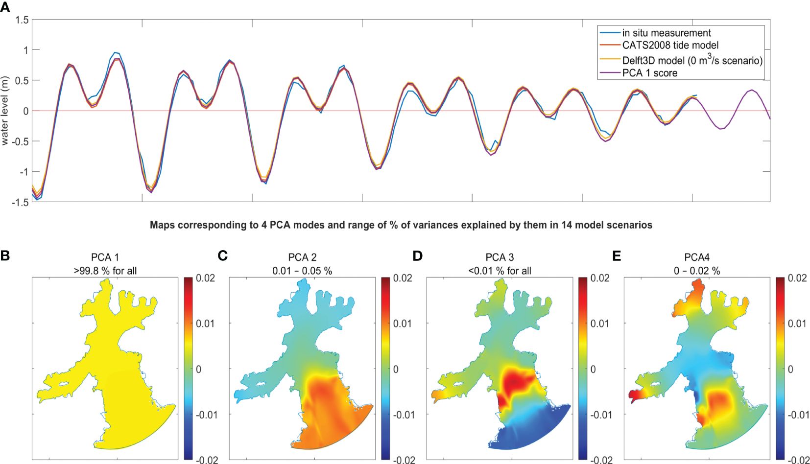
Figure 6 Results of PCA analysis of water level changes in 14 scenarios. (A) comparison of in situ water level measurements, CATS2008 tide model input data, Delft3D 0 m³/s model results and normalized PCA1 score (note that score values are non-dimensional, they have been divided by its double standard deviation to fit); (B–E) maps corresponding to first four principal components of water level 0 m³/s scenario (-); the percentages of water level variance explained by each mode in fourteen scenarios are shown above each map.

Tides are a primary driver of water level fluctuations in AB. This is demonstrated in Figure 6A where a comparison of in situ measurements collected by RBR wavemeter moored 9.5 km away from the AB outlet (location marked in Figure 1A) with tidal data from CATS2008 at the open boundary of the Delft3D model is shown. The blue line corresponding to in situ measurements exhibits only small deviations from modeled data, presumably during periods of very strong winds. The yellow line represents Delft3D model results at the grid point closest to the wavemeter location. The very good agreement between the three curves shows that the water level in the whole AB reacts almost instantaneously to the open boundary forcing.

PCA analysis of water level in the 0 m³/s scenario further confirms almost instantaneous response of the whole AB to tidal shifts. Figures 6B–E shows maps of coefficients corresponding to the first four PCA modes and the percentage of water level variance explained by them, respectively. The first PCA mode (PCA 1), which represents homogenous changes in the water level of the whole AB, explains more than 99.8% of the variance in all studied scenarios. Accordingly, the PCA 1 score correlates almost perfectly with the time series of water level at the boundary and inside of the model domain (see time series in Figure 6A). This indicates that anomalies from this pattern are of the order of a hundredth of a percentage, even in the 60 m³/s scenario, in which an additional 2000 m³ of water is pumped into AB every second. The predominance of tidal impact on water level changes is not surprising, since volume flux through the open boundary is of the order of 100,000 m³/s.

Although explaining small percentages of variance, other PCA modes of water level shifts are showing important characteristics of water level fluctuations in AB. Modes 2-4 represent standing-wave-like water level fluctuations with respectively one, two, and three nodes (Valle-Levinson, 2022). Each of the maps in Figures 6B–E emphasizes a region in central AB that corresponds to the location of a smaller circulation cell in the overall AB circulation pattern (Section 4.1.2 and Figure 7).

Figure 7

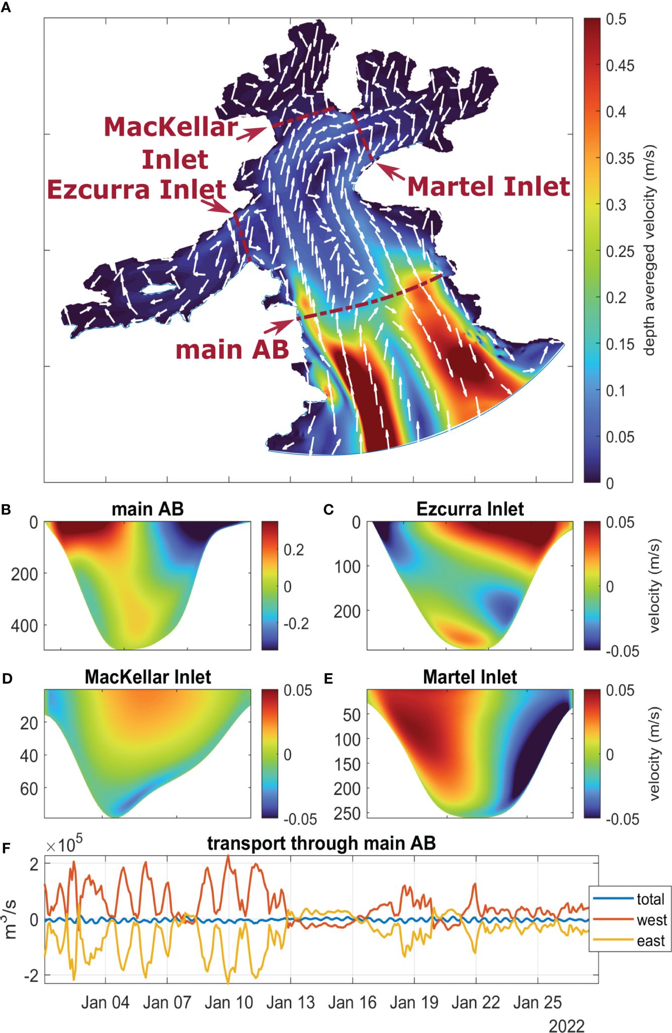
Figure 7 General circulation pattern of AB without glacial influx; (A) horizontal flow depth averaged velocities (map colors) and directions (white arrows); (B–E) horizontal velocities across four crossections (their location in Figure 7A, positive values correspond to inflow into inlets, negative to outflow; (F) transport through main AB crossection, total (blue line) and divided into western (red line) and eastern half (yellow line). Values in (A–E) are average for the period 1.01.2022-28.01.2022.

3.1.2 Changes in circulation and freshwater distribution

The most notable feature of AB general circulation is a strong northerly flow along its western boundary (Figure 7A). It is formed by the Coriolis force acting upon Bransfield Strait waters flowing northeast along the edge of the South Shetland Islands (Zhou et al., 2002). The existence of this current was recognized by prior modeling conducted in the AB by (Robakiewicz and Rakusa-Suszczewski, 1999). Following its initial development, the AB inflow current continues in a northerly direction and subsequently undergoes bifurcation. Part of it flows to the right in the central region of the main body of the AB, approximately 7 km from the AB outlet (around the location of main AB cross-section), and then exits the bay in close proximity to its eastern boundary. The second limb of the current penetrates deeper before reversing its course in the main embranchment of the bay (~13.5 km from the opening) and also flows back to the bay opening along its eastern coast. The clockwise (cyclonic) circulation cells formed by these two branches are crucial elements of the water exchange mechanism between the ocean and inner bay waters. A visualization of monthly average velocities across the main AB cross-section (Figure 7B) reveals that this exchange has the greatest magnitude in the surface layer. In the scenario without glacial influx there exists a state of equilibrium between the amount of water flowing into AB via its western half and the amount flowing out of it through the eastern half of the main AB cross-section (Figure 7F). At spring tide, the volume of water transported through each of the halves reaches 2·10⁵ m³/s. The quantities of water penetrating the three inner inlets of AB, Ezcurra, MacKellar, and Martel Inlet are two orders of magnitude smaller, with proportionally lower velocities observed across their respective cross-sections (Figures 7C–E).

When glacial influx is introduced, AB’s cyclonic circulation explains the development of distinct patterns in glacial water dispersal, illustrated by FWT and pycnocline depth maps (Figure 8). In each of the model scenarios, following an initial warm-up period, a quasi-stationary state is reached, in which the distribution of FWT remains approximately constant (Supplementary Figure 4). With rising glacial influx levels, freshwater accumulates in the northeastern region of AB, specifically in MacKellar and Martel Inlets. This freshwater is then transported to Bransfield Strait by the AB’s eastern outflowing current. In the accumulation zones, the FWT values range from 0 to 0.5 m. The FWT exceeds 1 m in larger areas only in the two strongest glacial influx scenarios, 28 m³/s and 60 m³/s. The increase of glacial input results in the expansion of the region where the pycnocline occurs, as well as in its deepening. The pycnocline depth is determined by the local bathymetry, resulting in the deepest pycnocline developing in the area of the main AB embranchment. In all scenarios, the depth of the pycnocline does not exceed 60 m.

Figure 8

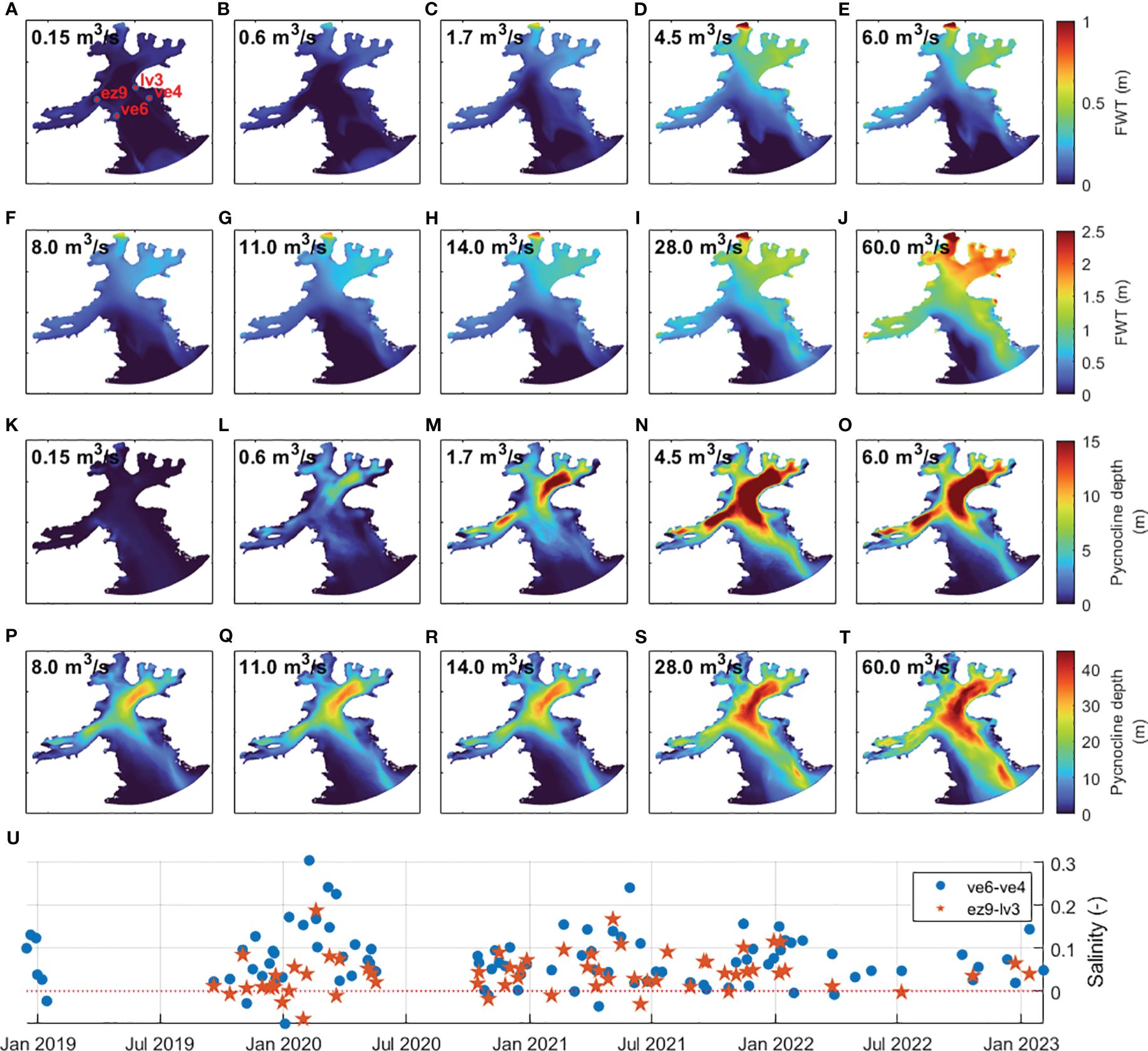
Figure 8 Variability of FWT and pycnocline depth with increasing glacial input; (A–J) FWT; (K–T) pycnocline depth. Note changing scales in different rows; (U) difference in average salinity readings from top 60 m of inflow (ve6 and ez9) and outflow (ve4 and lv3) sites [sites’ locations seen in (A)] Values in (A–T) are average for the period 1.01.2022-28.01.2022.

The model results demonstrate circulation and freshwater distribution patterns that are consistent with the in situ measurement data. The average salinity values from the top 60 m of water at two sites in the western inflow area, ve6 and ez9, consistently exceed those reported at the outflow sites, ve4 and lv3. Despite the close proximity and similar distance from the glacial front and bay’s outlet between inflow and outflow sites, this salinity difference can reach 0.3 (Figure 8U and Figure 8A for).

In all the model scenarios, the circulation pattern of two cyclonic circulation cells is preserved in AB (Figures 9A–E). The analysis of flow velocities and transport volumes across the main AB cross-section reveals that in scenarios ranging from 0 to 14 m³/s, the water exchange is consistently strongest near the surface and has a volume of ~10⁵ m³/s for both inflow and outflow (Figures 9F–J, and Figure 9Z, analogous to Figures 7B, F). However, in two highest glacial influx scenarios (28 and 60 m³/s), the water transport on both sides of the main AB cross-section decreases significantly to ~10⁴ m³/s (Figure 9Z). Similarly, in these scenarios, the flow velocities are reduced (see Figures 9E, J). This observation suggests that a threshold value of glacial inflow volume exists limiting water interchange between the bay and the ocean. Specifically this threshold is observed to be between 14 and 28 m³/s ~1 km of glacial front, which adds up to 450 and 900 m³/s of overall freshwater input into AB.

Figure 9

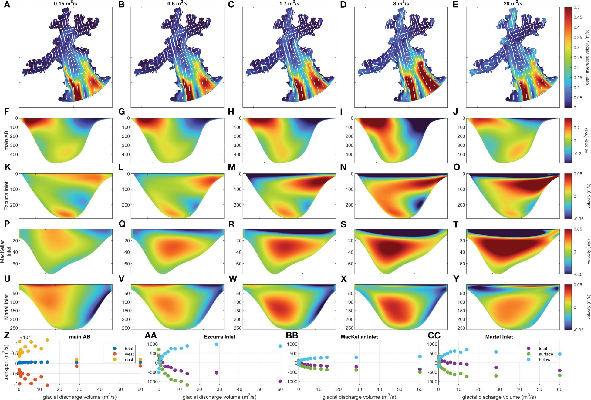
Figure 9 AB circulation influenced by growing glacial influx (five chosen model scenarios’ results); (A–E) flow depth averaged horizontal velocities in whole AB; (F–Y) horizontal velocity throughout cross-sections (locations in Figure 7A); (Z) variability in mean transport through cross-section main AB in total and divided into western and eastern half; (AA–CC) variability in transport through AB inlets: total and divided into surface and below surface layers; for (F–CC) positive values =inflow, negative =outflow. All values are average for the period 1.01.2022-28.01.2022.

In cross-sections located at the openings of inner AB inlets, Ezcurra, MacKellar, and Martel Inlets, the impact of increasing glacial influx is visible from relatively low glacial water inflow rates below 0.6 m³/s, (Figures 9F–Y). The surface outflow layer forms there, moving GMW out of the bay, most evidently in the Ezcurra and MacKellar Inlets (Figures 9K–T). Figures 9AA–CC shows the variability in water volume transported through the three inlet cross-sections in 14 model scenarios, in total, and split into layers above (surface layer) and below the pycnocline depth (calculated as in section 3.3.2). In AB inlets, surface outflow and deeper inflow increase with rising glacial influx, up to 14 m³/s scenario, when their values stabilize. This demonstrates how glacial influx drives vertical circulation, similar to the 2D glacial bay circulation of (Motyka et al., 2003). The drop in total transport values in Figures 9AA–CC indicates the importance of additional freshwater input for the water budget of AB inner inlets, which is barely visible in the flow transport sum up through the main AB cross-section, where overall values are 100 times higher (Figure 9Z).

Maps depicting the correlation coefficients between the glacial influx volumes and horizontal flow velocities and directions have been generated (Figure 10). They show areas in which glacial bay buoyancy-driven vertical circulation can be a dominant flow pattern. The maps are shown in three versions: for the entire water column, for depths below the pycnocline, and for surface waters inside and above the pycnocline. In regions where pycnocline was not present, the entire column of water was treated as waters below the pycnocline. In order to acquire representative description of changes in waters above pycnocline (Figures 10C, F), correlations have been calculated for points in which pycnocline was present in at least six model scenarios. To reduce the possible influence of outliers and increase the robustness of the results, a bootstrap resampling of the data was performed (Trauth, 2010). The areas outlined with black borders in all of the maps in Figure 10 represent points where this analysis produced statistically significant results.

Figure 10

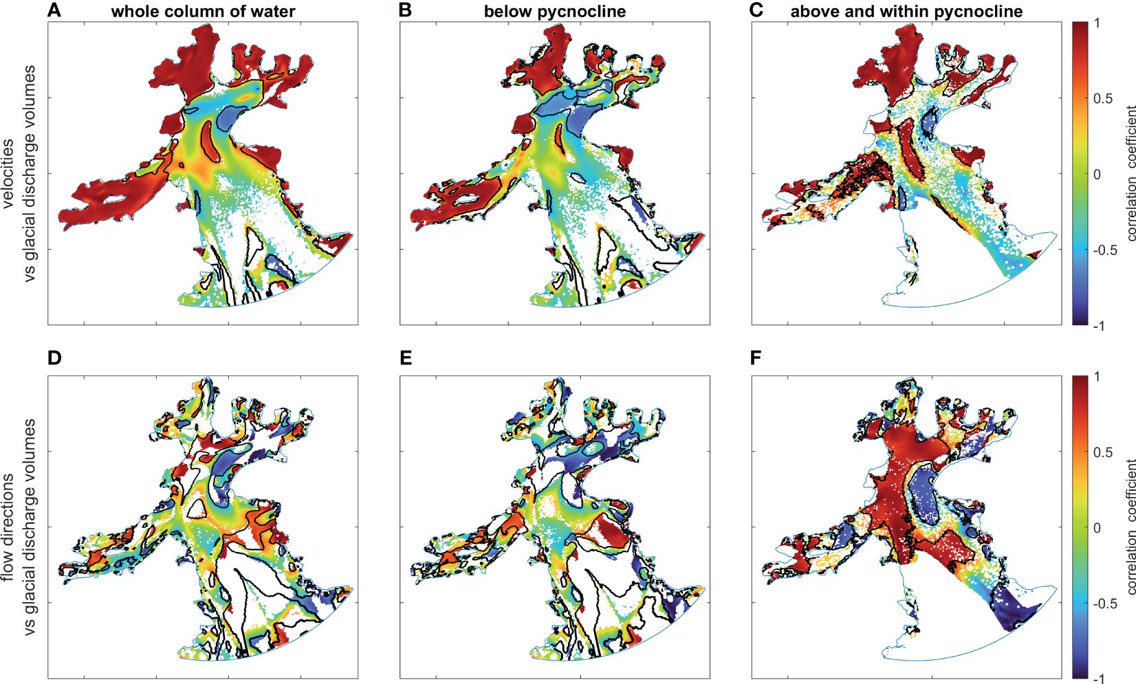
Figure 10 Correlation between rising glacial influx and flow horizontal velocities and directions; (A–C) correlation coefficients between flow velocities and glacial discharge volumes; (D–F) correlation coefficients between flow directions and glacial discharge volumes; positive values correspond to flow turning to the right, negative to the left; (A, D) average value over the water column; (B, E) below pycnocline; (C, F) above and within pycnocline. Areas within black boundaries contain statistically significant values.

In three inner AB inlets, the whole of Ezcurra and MacKellar Inlets, and most of Martel Inlet, there is a strong correlation between horizontal flow velocity and glacial influx (Figures 10A–C). Overall, based on the evidence in Figures 9, 10, we conclude that in these areas glacial input can create vertical circulation, driving local water exchange.

In the entire water column and in the bottom layers, the distributions of correlation coefficients of flow direction changes versus glacial influx volumes do not show any discernible pattern (Figures 10D–E). However, in the surface waters, a distinct areas can be recognized where, with rising glacial input, water flow turns to the right in a broad area in the middle of AB and to the left in a smaller area in the east part of the main embranchment of AB (Figure 10F). This shows how the GMW surface layer deflects surface water following the general circulation pattern (Figure 7A), redirecting it toward the AB outlet and restricting its penetration of inner bay waters.

3.2 Assessment of seasonal variability in glacial influx volume

Ice mass balance models, such as the Regional Atmospheric Climate Model (RACMO2, Wessem and Laffin, 2020), are commonly used to predict glacial influx volumes (Xu et al., 2012; Mankoff et al., 2016). However, due to its coarse scale in both time and space, as well as considerable uncertainty in its results (Mernild et al., 2010; Cape et al., 2019), a more locally conformable method has been developed.

Estimates of glacial input volume into AB were obtained by comparing FWT values from hydrographic observations to FWT values from 14 model scenarios, at grid points nearest to measurement site locations. A best-fitting scenario was identified for each site, per measurement day, as one with the smallest FWT difference from the FWT in measurement. The results for each day were summarized in a boxplot (Figure 11), displaying a range in glacial influx volumes of best-fitting scenarios for each day across all locations.

Figure 11

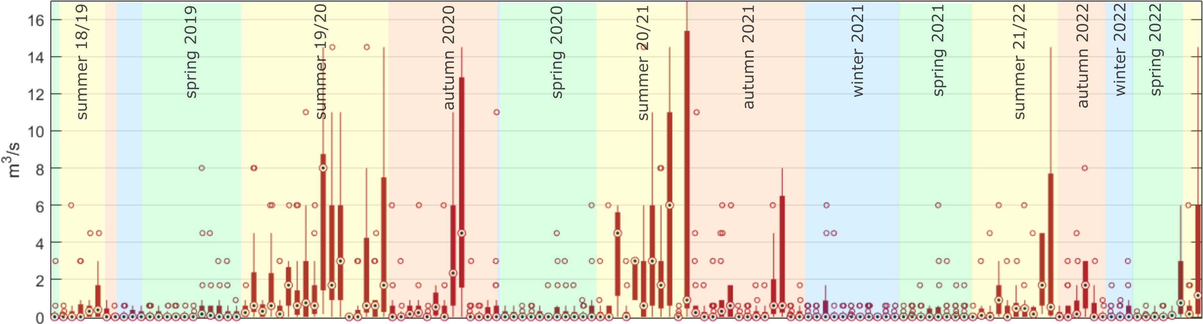
Figure 11 Estimation of glacial influx into AB assessed via a comparison of modeling and hydrographic measurement results; Glacial influx volume of scenarios with the smallest FWT difference from the measurement FWT (best-fitting scenario), in each boxplot information from all sites per measurement day (central mark=median, bottom and top edges of the box=25^th and 75^th percentiles, whiskers=extreme points, circles=outliers);.

Figure 11 shows that the range of glacial discharge volumes employed in modeling was reasonable: the maximum glacial influx scenario of 60 m³/s never fits best to observed results, and the second greatest scenario of 28 m³/s fits best once. Figure 11 depicts how winter and spring glacial influx values are close to 0 m³/s, while continuous highest discharge volumes occur in late summer and autumn, reaching a maximum daily median value of 8 m³/s. The median value of projected glacial influx volume is comparatively low, maximally 1.06-1.30 m³/s in the summer (Table 1). This observation implies that periods characterized by significant glacial influx are of limited duration.

Table 1

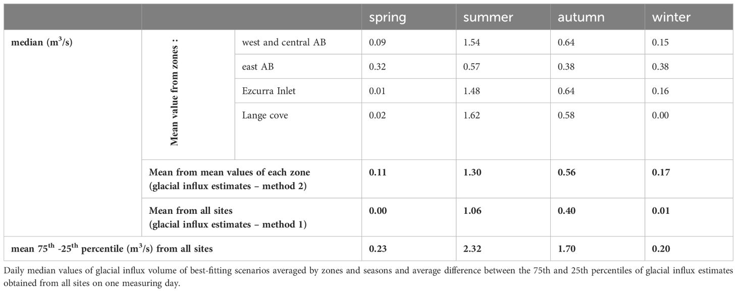
Table 1 Statistics of glacial influx estimation results.

Table 1 contains the seasonally averaged differences between the 75th and 25th percentiles of glacial influx estimates obtained from all sites on one measuring day. Their high values, particularly during the summer (2.32 m³/s), imply that the model does not accurately capture details of circulation in AB. The disparities between model and measurements might be caused by the unrealistic assumption of homogeneous and constant volumes of injections from all glaciers, by not taking into account the contribution of other freshwater sources and/or effects of wind-induced circulation. Nonetheless, the low glacial influx values of the best fitting model scenarios in the winter and spring (mean daily median of 0.01 and 0.00 m³/s, respectively) would suggest that the omission of precipitation and sea ice contribution was reasonable.

In general, the measurements confirm the overall circulation pattern of AB that was identified through modeling. This was first shown in salinity differences between west and east sites in Figure 8U. Through the course of the study period, the FWT in east AB, in the area of GMW outflow, was no thicker than 0.35 m (0.05-0.35 m - measurements, 0.00-0.27 m - modelling). The difference between the FWT values in east AB and west and central AB sites varied from -0.04 to 0.21 m (difference between the red and blue plot in Figure 4), which indicates the creation of a surface GMW outflow layer along the eastern boundary. Accordingly, the difference in FWT from analogous model points in a timeseries generated from the daily median of the best-fit scenarios shown in Figure 11 was in the range of 0.00–0.14 m, i.e., the model tends to underestimate the observed west-east FWT differences, but reproduces the overall pattern.

The daily estimate of glacial influx was defined as the median of the glacial influx volumes of the best-fit scenario from all sites on one day. Seasonal glacial influx values were obtained using two methods (Table 1): 1. Calculating the seasonal mean of all daily glacial influx estimates; 2. Calculating the seasonal means for each of the four zones, and then averaging these four values. The difference in results from these two methods established a range of seasonal glacial influx estimates. Based on these results glacial discharge per ~1 km of glacial front in AB is estimated to be between 0.01-0.17 m³/s in winter, 0.00 to 0.11 m³/s in spring, 1.06-1.30 m³/s at its peak in summer, and 0.40-0.56 m³/s in fall. Therefore, the volume of glacial water released from all the glaciers into AB is valued to be in the range 0.434-0.632 Gt/year (0.104-0.128 Gt/month in summer, 0.039-0.55 Gt/month in autumn, 0.001-0.016 Gt/month in winter, and 0.000-0.010 Gt/month in spring).

4 Discussion and conclusions

A novel method of estimating glacial influx volume has been implemented and evaluated. This methodology uses a comparison of hydrographic measurements and modeling results, utilizing an extensive dataset to affirm the validity of its findings. Other studies estimating glacial influx quantities frequently employed far fewer observational data than the 1830 measurements used in this study (Mortensen et al., 2013; Sutherland et al., 2014; Straneo and Cenedese, 2015).

The scale of the analysis is critical when examining ocean-cryosphere interactions. Straneo and Cenedese (2015) defined three glacial bay regions: the ice-ocean boundary zone, the glacial plume region, and the major fjord system. The current research focuses on AB hydrodynamics at this third scale. In this broad perspective, the vertical placement of glacial discharges and their initial velocity has no significant impact on the overall AB circulation. This conclusion could help investigate the hydrodynamics of other similar bays in the WAP region.

Based on all hydrographic measurements and model results the standard deviation of salinity was 0.22 and the standard deviation of water temperature was 0.90°C in AB (Figure 2 and Supplementary Figure 1). GMW has always been the most buoyant water mass, occurring at the surface of the water column, spreading in a distinctive pattern along the eastern boundary of AB, generated by the AB general circulation pattern. The freshwater content in the GMW outflow area is low throughout the year, the maximal FWT in the east AB zone was 0.27-0.35 m. The temperature of glacial water exhibits slight variations compared to AW, being either colder or warmer than AW at the moment of discharge. The GMW surface layer can undergo either warming or cooling as a consequence of atmospheric forcing, dependent on the air temperature.

By integrating the findings of glacial influx estimation from Section 4.2 with the analysis of the impact of different volumes of glacial discharge on water level shifts and circulation from Sections 4.1.1 and 4.1.2, it can be inferred that glacial influx does not alter the general hydrodynamics of AB. The double-celled horizontal circulation pattern, which regulates water exchange between AB and the ocean, has been observed to persist consistently throughout the year. Unlike the findings of Mortensen et al. (2013) and Straneo et al. (2011) in Greenland, no distinct modes of circulation specific to different seasons were identified in the whole AB. However, in the Ezcurra, MacKellar, and inner parts of Martel inlets, the presence of GMW can lead to the formation of buoyancy-driven vertical circulation. This circulation is expected to occur most of the time during the summer and beginning of the autumn (estimates of glacial input > 0.6 m³/s) and to be particularly robust during short-term peak melt events (Figures 9, 11).

It is suspected that there exists a threshold volume of glacial influx, estimated to be within the range of 14 to 28 m³/s ~ per 1 km of a glacial front. GMW is expected to significantly limit the interchange of water between the AB and the ocean above this threshold (Figures 9Z–CC), since the ocean induced general circulation in the AB is most intense at the surface, at the level in which GMW is transported outside AB. The estimated amounts of glacial influx did not reach this level at any given time of the analyzed period. The likelihood of such high glacial influx levels requires further inquiry, however it is outside of the scope of this investigation.

The current investigation uncovered key features of AB hydrodynamics (visualized in Figure 12), that set it apart from the better-studied fjords of the northern hemisphere. These differences are caused by the geomorphology of the region and different relative contributions of external forces acting upon the bay waters. Similar geomorphological, oceanographic and meteorological conditions can be found at other locations in South Shetlands, like the nearby Maxwell Bay, where the Mariana and Potter Coves may have a similar function to that of Admiralty Bay’s inner inlets. Similarly to AB, no evidence of CDW incursions has been found in Maxwell Bay, and glacial water was only present in the top layers of the water column (Meredith et al., 2018; Jones et al., 2023).

Figure 12

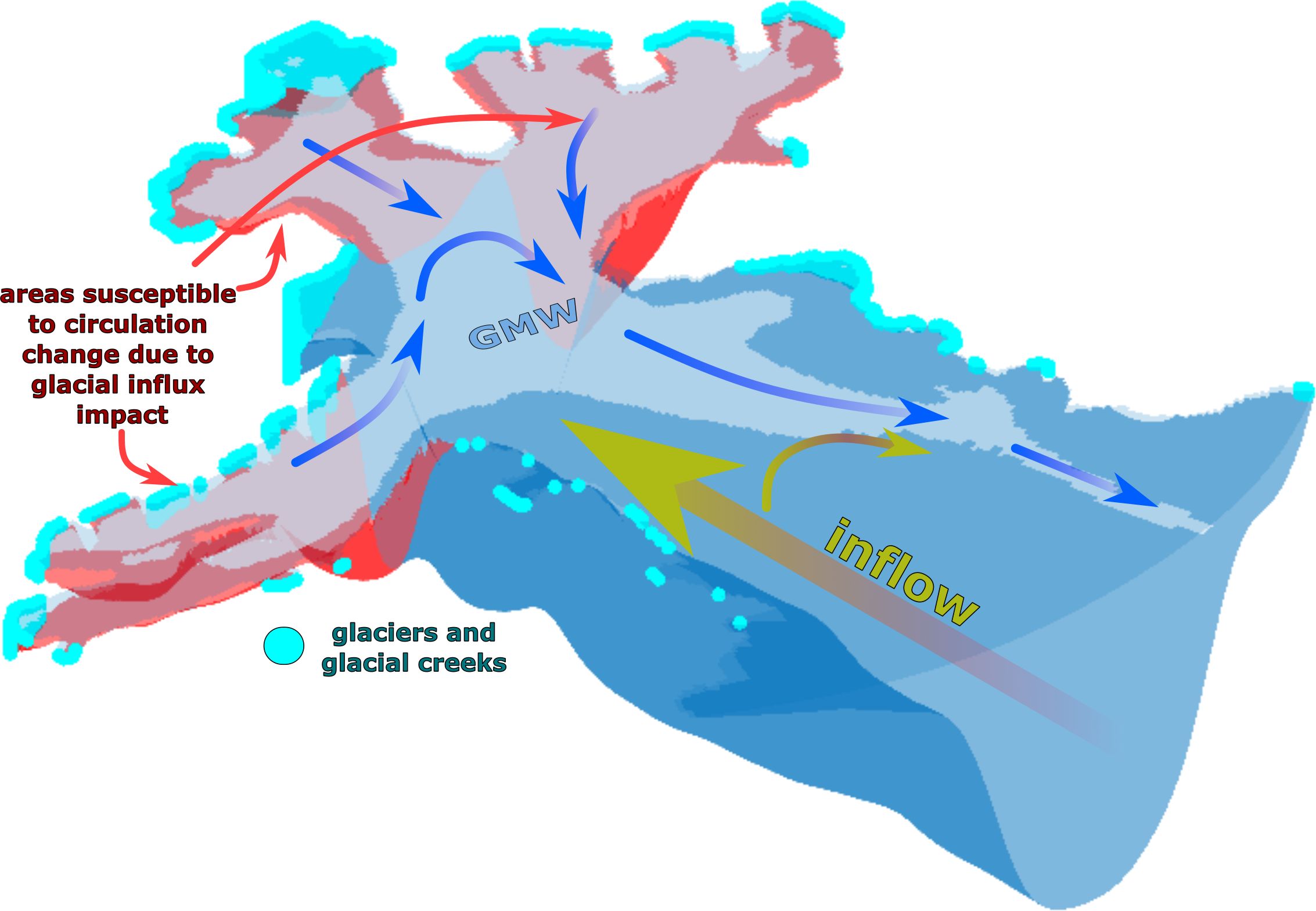
Figure 12 Key feature of Admiralty Bay hydrodynamics.

To estimate the significance of the study’s findings for the Antarctic Peninsula’s bays, a more detailed comparison between them and AB must be given. In terms of scale, the AB (area = 150 km²) is within the range of sizes found in WAP, e.g.: Andvord Bay has an area of 110 km², Barilari Bay 280 km², Flandres Bay 310 km², Charlotte Bay 110 km², Beascochea Bay 200 km². In addition, these bays are wide and have deeper sills than fjords in the northern hemisphere. This would suggest that rotational forces are important in all of them, just like in AB. Furthermore, its topography, with multiple inlets extending from the main bay, implies that there may be regions in which glacial inflow has the potential to alter local hydrodynamics and to create vertical circulation patterns.

However, there are a few significant differences between AB and the bays along the WAP. The AB ice-water boundaries take up 25% of its overall coastline length, in WAP this percentage is usually higher. In addition, AB glaciers are shallower and smaller. For instance, grounding depths of four glaciers in Barilari Bay range from 168 to 367 m (Cape et al., 2019) compared to the maximal glacial grounding depth of 150 m in AB. Furthermore, CDW intrusions are more common further south along the Antarctic Peninsula. These intrusions might enhance faster melt rates of more deeply submerged glacial fronts, which can have a significant impact on local circulation (Meredith et al., 2010; Cape et al., 2019).

Katabatic wind events and precipitation—both of which are influenced by the high orography—play a more significant impact in the Antarctic Peninsula than in KGI (Cape et al., 2019; Lundesgaard et al., 2019). The entire region is susceptible to climate change (Bers et al., 2013) and extreme warm weather events have been reported, such as in February 2022 when temperatures above 10°C were recorded throughout WAP and South Shetlands (Gorodetskaya et al., 2023). These events are predicted to become more frequent in the future. Lastly, the sea ice presence is still a common occurrence along the WAP coast, so that freezing and melting influence local freshwater content variability.

It is important to thoroughly assess all of the aforementioned aspects before extending the techniques and conclusions from this study to other WAP locations. However, despite these differences, the glacial input estimates are in the same range in the whole region. The volume of glacial water released into AB during the summer is estimated to be in the range 0.104-0.128 Gt/month, in Andvord Bay, smaller than AB, it is 0.128 Gt/month, and 0.167 Gt/month in a larger Barilari Bay (Cape, et al. 2019; Hahn-Woernle et al., 2020).

All of these estimates are significantly lower than the glacial fluxes estimated for northern hemisphere fjords (Mernild et al., 2010; De Andrés et al., 2020). In Spitsbergen, the percentage share of glacial freshwater in the overall bay water budget was estimated to be around 1% (Cottier et al., 2010), in model-based study of Greenland fjords it was up to 0.25% (Cowton et al., 2015). In the summer, on average, the glacial freshwater contribution to the AB water budget is in the range of 0.19 to 0.23% (0.9–1.7 m3/s scenario results; see Supplementary Figure 5). Also, FWT in AB is lower than in, for example, Sermilik and Kangerdlugaauqq Greenlandic fjords, where in the summer it consistently exceeded 10 m (Sutherland et al., 2014), whereas in AB, even in the unrealistic maximum glacial influx scenarios, it seldom exceeded 3 m. This is due to relatively low glacial input volumes, as well as ocean-driven circulation that carries GMW out of AB in a thin surface layer, a phenomenon observed in other Antarctic bays by Hahn-Woernle et al. (2020) and Meredith et al. (2018).

Notably all of the previous estimates of glacial influx into the WAP bays concern summer months. Our study have provided first ever results showing its year-round variations. In AB the estimated glacial influx volumes rise more than ten times between spring/winter season and summer. These significant seasonal variations can be attributed to the absence of external warm water masses stimulating submarine melt during austral winter, a process demonstrated in studies conducted in Greenlandic fjords (Straneo et al., 2011; Mortensen et al., 2013) and in WAP region (Cook et al., 2016; Cape et al., 2019). This variability may also be exacerbated by the fact that the majority of the AB glaciers are shallowly grounded, causing melt to be primarily driven by external heat rather than hydrostatic pressure (Jenkins, 2011).

This study provides a comprehensive analysis of the hydrodynamic response of an Antarctic bay to changes in magnitude of glacial influx. Furthermore, with a large number of data points and high temporal resolution, this study offers, to the best of our knowledge, the most comprehensive assessment of seasonal variations in glacial discharge volumes to date. This enables the prediction of variations in circulation within a glacial bay over the course of a year.

Data availability statement

The datasets presented in this study can be found in online repositories. The names of the repository/repositories and accession number(s) can be found below: PANGAEA: https://doi.org/10.1594/PANGAEA.947909; Zenodo: 10.5281/zenodo.10277429; Zenodo 10.5281/zenodo.10277333.

Author contributions

MO: Conceptualization, Data curation, Formal analysis, Investigation, Methodology, Software, Validation, Visualization, Writing – original draft, Writing – review and editing. AH: Conceptualization, Funding acquisition, Methodology, Project administration, Resources, Supervision, Writing – review and editing.

Funding

The author(s) declare financial support was received for the research, authorship, and/or publication of this article. This work was supported by two grants from the National Science Centre, Poland: No. 2017/25/B/ST10/02092 ‘Quantitative assessment of sediment transport from glaciers of South Shetland Islands on the basis of selected remote sensing methods’ and No. 2018/31/B/ST10/00195 ‘Observations and modeling of sea ice interactions with the atmospheric and oceanic boundary layers’.

Acknowledgments

Special thanks are owed to Laboratory of Sedimentary and Environmental Processes - INCT-Criosfera Fluminense Federal University - Geoscience Institute in Brazil for providing us with bathymetric data from Admiralty Bay, described in (Magrani et al., 2016). We are thankful to Deltares for making Delft3D Flow model available for calculations. Calculations were made possible thanks to computing power and software provided by CI TASK (Center of the Tri-City Academic Computer Network) in Gdańsk, Poland. We are grateful for the support of Arctowski Polish Antarctic Station’s crew for all their help during measurement campaign.

Conflict of interest

The authors declare that the research was conducted in the absence of any commercial or financial relationships that could be construed as a potential conflict of interest.

Publisher’s note

All claims expressed in this article are solely those of the authors and do not necessarily represent those of their affiliated organizations, or those of the publisher, the editors and the reviewers. Any product that may be evaluated in this article, or claim that may be made by its manufacturer, is not guaranteed or endorsed by the publisher.

Supplementary material

The Supplementary Material for this article can be found online at: https://www.frontiersin.org/articles/10.3389/fmars.2024.1365157/full#supplementary-material

References

Bartholomaus T. C., Larsen C. F., OʼNeel S. (2013). Does calving matter? Evidence for significant submarine melt. Earth Planet Sci. Lett. 380, 21–30. doi: 10.1016/j.epsl.2013.08.014

CrossRef Full Text | Google Scholar

Battke Z. (1990). Admiralty bay, king george island 1:50.000 map. Insitute Ecol. PAS.

Google Scholar

Bers A. V., Momo F., Schloss I. R., Abele D. (2013). Analysis of trends and sudden changes in long-term environmental data from King George Island (Antarctica): Relationships between global climatic oscillations and local system response. Clim. Change 116, 789–803. doi: 10.1007/s10584-012-0523-4

CrossRef Full Text | Google Scholar

Cape M. R., Vernet M., Pettit E. C., Wellner J., Truffer M., Akie G., et al. (2019). Circumpolar deep water impacts glacial meltwater export and coastal biogeochemical cycling along the west Antarctic Peninsula. Front. Mar. Sci. 6. doi: 10.3389/fmars.2019.00144

CrossRef Full Text | Google Scholar

Carbotte S. M., Ryan W. B. F., Hara S. O., Arko R., Goodwillie A., Melkonian A., et al. (2007). Antarctic multibeam bathymetry and geophysical data synthesis : An on-line digital data resource for marine geoscience research in the Southern Ocean. 10th Int. Symposium Antarctic Earth Sci. 196. doi: 10.3133/ofr20071047SRP002

CrossRef Full Text | Google Scholar

Carroll D., Sutherland D. A., Hudson B., Moon T., Catania G. A., Shroyer E. L., et al. (2016). The impact of glacier geometry on meltwater plume structure and submarine melt in Greenland fjords. Geophys Res. Lett. 43, 9739–9748. doi: 10.1002/2016GL070170

CrossRef Full Text | Google Scholar

Chauché N., Hubbard A., Gascard J. C., Box J. E., Bates R., Koppes M., et al. (2014). Ice-ocean interaction and calving front morphology at two west Greenland tidewater outlet glaciers. Cryosphere 8, 1457–1468. doi: 10.5194/tc-8-1457-2014

CrossRef Full Text | Google Scholar

Clarke A., Meredith M. P., Wallace M. I., Brandon M. A., Thomas D. N. (2008). Seasonal and interannual variability in temperature, chlorophyll and macronutrients in northern Marguerite Bay, Antarctica. Deep Sea Res. 2 Top. Stud. Oceanogr. 55 (18–19), 1988–2006. doi: 10.1016/j.dsr2.2008.04.035

CrossRef Full Text | Google Scholar

Cook A. J., Holland P. R., Meredith M. P., Murray T., Luckman A., Vaughan D. G. (2016). Ocean forcing of glacier retreat in the western Antarctic Peninsula. Sci. (1979) 353, 283–286. doi: 10.1126/science.aae0017

CrossRef Full Text | Google Scholar

Cottier F. R., Nilsen F., Skogseth R., Tverberg V., Skarthhamar J., Svendsen H. (2010). Arctic fjords: a review of the oceanographic environment and dominant physical processes. Geological Society London Special Publications 344, 35–50. doi: 10.1144/SP344.4

CrossRef Full Text | Google Scholar

Cowton T., Slater D., Sole A., Goldberg D., Nienow P. (2015). Modeling the impact of glacial runoff on fjord circulation and submarine melt rate using a new subgrid-scale parameterization for glacial plumes. J. Geophys Res. Oceans 120 (2), 796–812. doi: 10.1002/2014JC010324

CrossRef Full Text | Google Scholar

De Andrés E., Slater D. A., Straneo F., Otero J., Das S., Navarro F. (2020). Surface emergence of glacial plumes determined by fjord stratification. Cryosphere 14, 1951–1969. doi: 10.5194/tc-14-1951-2020

CrossRef Full Text | Google Scholar

Deltares (2020). Delft3D 3D/2D modelling suite for integral water solutions Hydro-Morphodynamics. User Manual, 1–701.

Google Scholar

Dotto T. S., Mata M. M., Kerr R., Garcia C. A. E. (2021). A novel hydrographic gridded data set for the northern Antarctic Peninsula. Earth Syst. Sci. Data 13, 671–696. doi: 10.5194/essd-13-671-2021

CrossRef Full Text | Google Scholar

Eayrs C., Li X., Raphael M. N., Holland D. M. (2021). Rapid decline in Antarctic sea ice in recent years hints at future change. Nat. Geosci. 14 (7), 460–464. doi: 10.1038/s41561-021-00768-3

CrossRef Full Text | Google Scholar

Forsch K. O., Hahn-Woernle L., Sherrell R. M., Roccanova V. J., Bu K., Burdige D., et al. (2021). Seasonal dispersal of fjord meltwaters as an important source of iron and manganese to coastal Antarctic phytoplankton. Biogeosciences 18, 6349–6375. doi: 10.5194/bg-18-6349-2021

CrossRef Full Text | Google Scholar

Gerrish L., Fretwell P., Cooper P. (2021). High resolution vector polylines of the Antarctic coastline (7.4) [Data set]. (Cambridge, UK: British Antarctic Survey). doi: 10.5285/e46be5bc-ef8e-4fd5-967b-92863fbe2835

CrossRef Full Text | Google Scholar

Gorodetskaya I. V., Durán-Alarcón C., González-Herrero S., Clem K. R., Zou X., Rowe P., et al. (2023). Record-high Antarctic Peninsula temperatures and surface melt in February 2022: a compound event with an intense atmospheric river. NPJ Clim. Atmos. Sci. 6. doi: 10.1038/s41612-023-00529-6

CrossRef Full Text | Google Scholar

Gregory J. M., White N. J., Church J. A., Bierkens M. F. P., Box J. E., Van Den Broeke M. R., et al. (2013). Twentieth-century global-mean sea level rise: Is the whole greater than the sum of the parts? J. Clim. 26 (13), 4476–4499. doi: 10.1175/JCLI-D-12-00319.1

CrossRef Full Text | Google Scholar

Hahn-Woernle L., Powell B., Lundesgaard Ø., van Wessem M. (2020). Sensitivity of the summer upper ocean heat content in a Western Antarctic Peninsula fjord. Prog. Oceanogr. 183, 102287. doi: 10.1016/j.pocean.2020.102287

CrossRef Full Text | Google Scholar

Hofmann E. E., Klinck J. M., Lascara C. M., Smith D. A. (2011). “Water mass distribution and circulation west of the Antarctic Peninsula and including Bransfield Strait.,” (Washington DC, USA: American Geophysical Union). doi: 10.1029/ar070p0061

CrossRef Full Text | Google Scholar

Holfort J., Hansen E., Østerhus S., Dye S., Jónsson S., Meincke J., et al. (2008). “Freshwater fluxes east of Greenland,” in Arctic–Subarctic Ocean Fluxes (Springer Netherlands, Dordrecht), 263–287. doi: 10.1007/978-1-4020-6774-7_12

CrossRef Full Text | Google Scholar

Inall M. E., Rippeth T. P. (2002). Dissipation of tidal energy and associated mixing in a wide fjord. Environ. Fluid Mechanics 2 (3), 219–240. doi: 10.1023/A:1019846829875

CrossRef Full Text | Google Scholar

IPCC (2022). “Sea level rise and implications for low-lying islands, coasts and communities,” in The Ocean and Cryosphere in a Changing Climate (Cambridge UK: Cambridge University Press). doi: 10.1017/9781009157964.012

CrossRef Full Text | Google Scholar

Jenkins A. (1999). The impact of melting ice on ocean waters. J. Phys. Oceanogr 29 (9), 2370–2381. doi: 10.1175/1520-0485(1999)029<2370:TIOMIO>2.0.CO;2

CrossRef Full Text | Google Scholar

Jenkins A. (2011). Convection-driven melting near the grounding lines of ice shelves and tidewater glaciers. J. Phys. Oceanogr. 41, 2279–2294. doi: 10.1175/JPO-D-11-03.1

CrossRef Full Text | Google Scholar

Jenkins A., Jacobs S. (2008). Circulation and melting beneath George VI Ice Shelf, Antarctica. J. Geophys. Res. 113, C04013. doi: 10.1029/2007JC004449

CrossRef Full Text | Google Scholar

Jones R. L., Meredith M. P., Lohan M. C., Woodward E. M. S., Van Landeghem K., Retallick K., et al. (2023). Continued glacial retreat linked to changing macronutrient supply along the West Antarctic Peninsula. Mar. Chem. 251, 104230. doi: 10.1016/j.marchem.2023.104230

CrossRef Full Text | Google Scholar

Kimura S., Holland P. R., Jenkins A., Piggott M.. (2014). The Effect of Meltwater Plumes on the Melting of a Vertical Glacier Face. J. Phys. Oceanogr. 44 (12), 3099–3117. doi: 10.1175/JPO-D-13-0219.1

CrossRef Full Text | Google Scholar

Lundesgaard Ø., Powell B., Merrifield M., Hahn-Woernle L., Winsor P. (2019). Response of an antarctic peninsula fjord to summer katabatic wind events. J. Phys. Oceanogr. 49, 1485–1502. doi: 10.1175/JPO-D-18-0119.1

CrossRef Full Text | Google Scholar

Lundesgaard Ø., Winsor P., Truffer M., Merrifield M., Powell B., Statscewich H., et al. (2020). Hydrography and energetics of a cold subpolar fjord: Andvord Bay, western Antarctic Peninsula. Prog. Oceanogr. 181, 102224. doi: 10.1016/j.pocean.2019.102224

CrossRef Full Text | Google Scholar

Magrani F., Neto A. A., Vieira R. (2016). Glaciomarine sedimentation and submarine geomorphology in Admiralty Bay, South Shetland Islands, Antarctica. 2015 IEEE/OES Acoustics Underwater Geosciences Symposium Rio Acoustics 2015. doi: 10.1109/RIOACOUSTICS.2015.7473614

CrossRef Full Text | Google Scholar

Majdański M., Środa P., Malinowski M., Czuba W., Grad M., Guterch A., et al. (2008). 3D seismic model of the uppermost crust of the Admiralty Bay area, King George Island, West Antarctica. Polar Res. 29, 303–318.

Google Scholar

Mankoff K. D., Straneo F., Cenedese C., Das S. B., Richards C. G., Singh H. (2016). Structure and dynamics of a subglacial discharge plume in a Greenlandic fjord. J. Geophys Res. Oceans 121 (12), 8670–8688. doi: 10.1002/2016JC011764

CrossRef Full Text | Google Scholar

Meredith M. P., Falk U., Bers A. V., Mackensen A., Schloss I. R., Barlett E. R., et al. (2018). Anatomy of a glacial meltwater discharge event in an Antarctic cove. Philos. Trans. R. Soc. A: Mathematical Phys. Eng. Sci. 376 (2122), 20170163. doi: 10.1098/rsta.2017.0163

CrossRef Full Text | Google Scholar

Meredith M. P., King J. C. (2005). Rapid climate change in the ocean west of the Antarctic Peninsula during the second half of the 20th century. Geophys. Res. Lett. 32, n/a–n/a. doi: 10.1029/2005GL024042

CrossRef Full Text | Google Scholar

Meredith M. P., Wallace M. I., Stammerjohn S. E., Renfrew I. A., Clarke A., Venables H. J., et al. (2010). Changes in the freshwater composition of the upper ocean west of the Antarctic Peninsula during the first decade of the 21st century. Prog. Oceanogr. 87, 127–143. doi: 10.1016/j.pocean.2010.09.019

CrossRef Full Text | Google Scholar

Mernild S. H., Howat I. M., Ahn Y., Liston G. E., Steffen K., Jakobsen B. H., et al. (2010). Freshwater flux to sermilik fjord, SE Greenland. Cryosphere 4 (4), 453–465. doi: 10.5194/tc-4-453-2010

CrossRef Full Text | Google Scholar

Moffat C., Meredith M. (2018). Shelf–ocean exchange and hydrography west of the Antarctic Peninsula: a review. Philos. Trans. R. Soc. A: Mathematical Phys. Eng. Sci. 376, 20170164. doi: 10.1098/rsta.2017.0164

CrossRef Full Text | Google Scholar

Moffat C., Owens B., Beardsley R. C. (2009). On the characteristics of Circumpolar Deep Water intrusions to the west Antarctic Peninsula Continental Shelf. J. Geophys. Res. Oceans 114. doi: 10.1029/2008JC004955

CrossRef Full Text | Google Scholar

Monien D., Monien P., Brünjes R., Widmer T., Kappenberg A., Silva Busso A. A., et al. (2017). Meltwater as a source of potentially bioavailable iron to Antarctica waters. Antarct. Sci. 29, 277–291. doi: 10.1017/S095410201600064X

CrossRef Full Text | Google Scholar

Mortensen J., Bendtsen J., Lennert K., Rysgaard S. (2014). Seasonal variability of the circulation system in a west Greenland tidewater outlet glacier fjord, Godthåbsfjord (64°N). J. Geophys. Res.: Earth Surface 119 (12), 2591–2603. doi: 10.1002/2014JF003267

CrossRef Full Text | Google Scholar

Mortensen J., Bendtsen J., Motyka R. J., Lennert K., Truffer M., Fahnestock M., et al. (2013). On the seasonal freshwater stratification in the proximity of fast-flowing tidewater outlet glaciers in a sub-Arctic sill fjord. J. Geophys Res. Oceans. 118, 1382–1395. doi: 10.1002/jgrc.20134

CrossRef Full Text | Google Scholar

Motyka R. J., Hunter L., Echelmeyer K. A., Connor C. (2003). Submarine melting at the terminus of a temperate tidewater glacier, LeConte Glacier, Alaska, U.S.A. Ann. Glaciol. 36, 57–65. doi: 10.3189/172756403781816374

CrossRef Full Text | Google Scholar

National Snow and Ice Data Center, C. (2023). Sea Ice Index. Available at: https://nsidc.org/data/seaice_index (Accessed June 7, 2023).

Google Scholar

Naughten K. A., Holland P. R., De Rydt J. (2023). Unavoidable future increase in West Antarctic ice-shelf melting over the twenty-first century. Nat. Clim. Change 13 (11), 1222–1228. doi: 10.1038/s41558-023-01818-x

CrossRef Full Text | Google Scholar

Osińska M., Bialik R. J., Wójcik-Długoborska K. A. (2021). Interrelation of quality parameters of surface waters in five tidewater glacier coves of King George Island, Antarctica. Sci. Total Environ. 771, 144780. doi: 10.1016/j.scitotenv.2020.144780

PubMed Abstract | CrossRef Full Text | Google Scholar

Osińska M., Wójcik-Długoborska K. A., Bialik R. J. (2022). Water conductivity, salinity, temperature, turbidity, pH, fluorescent dissolved organic matter (fDOM), optical dissolved oxygen (ODO), chlorophyll a and phycoerythrin measurements in Admiralty Bay, King George Island, from Dec 2018 to Jan 2022. PANGAEA. doi: 10.1594/PANGAEA.947909

CrossRef Full Text | Google Scholar

Osińska M., Wójcik-Długoborska K. A., Bialik R. J. (2023). Annual hydrographic variability in Antarctic coastal waters infused with glacial inflow. Earth Syst. Sci. Data 15, 607–616. doi: 10.5194/essd-15-607-2023

CrossRef Full Text | Google Scholar

Padman L., Fricker H. A., Coleman R., Howard S., Erofeeva L. (2002). A new tide model for the Antarctic ice shelves and seas. Annals of Glaciology 34, 247–254. doi: 10.3189/172756402781817752

CrossRef Full Text | Google Scholar

Plenzler J., Budzik T., Puczko D., Bialik R. J. (2019). Climatic conditions at Arctowski Station (King George Island, West Antarctica) in 2013-2017 against the background of regional changes. Pol. Polar Res. 40, 1–27. doi: 10.24425/ppr.2019.126345

CrossRef Full Text | Google Scholar

Potapowicz J., Szumińska D., Szopińska M., Bialik R. J., Machowiak K., Chmiel S., et al. (2020). Seashore sediment and water chemistry at the Admiralty Bay (King George Island, Maritime Antarctica) – Geochemical analysis and correlations between the concentrations of chemical species. Mar. pollut. Bull. 152, 110888. doi: 10.1016/j.marpolbul.2020.110888

PubMed Abstract | CrossRef Full Text | Google Scholar

Poulin F. J., Stegner A., Hernández-Arencibia M., Marrero-Díaz A., Sangrà P. (2014). Steep shelf stabilization of the coastal bransfield current: Linear stability analysis. J. Phys. Oceanogr. 44 (2), 714–732. doi: 10.1175/JPO-D-13-0158.1

CrossRef Full Text | Google Scholar

Powell R., Domack G. W. (2002). Modern glaciomarine environments. Modern Past Glacial Environments, pp. 361–389. doi: 10.1016/B978-075064226-2/50015-5

CrossRef Full Text | Google Scholar

Robakiewicz M., Rakusa-Suszczewski S. (1999). Application of 3D circulation model to Admiralty Bay, King George Island, Antarctica. Pol. Polar Res. 20, 43–58.

Google Scholar

Rückamp M., Blindow N., Suckro S., Braun M., Humbert A. (2010). Dynamics of the ice cap on King George Island, Antarctica: Field measurements and numerical simulations. Ann. Glaciol. 51, 80–90. doi: 10.3189/172756410791392817

CrossRef Full Text | Google Scholar

Sangrà P., Gordo C., Hernández-Arencibia M., Marrero-Díaz A., Rodríguez-Santana A., Stegner A., et al. (2011). The Bransfield current system. Deep Sea Res. 1 Oceanogr Res. Pap. 58 (4), 390–402. doi: 10.1016/j.dsr.2011.01.011

CrossRef Full Text | Google Scholar

Schloss I. R., Abele D., Moreau S., Demers S., Bers A. V., González O., et al. (2012). Response of phytoplankton dynamics to 19-year, (1991–2009) climate trends in Potter Cove (Antarctica). J. Mar. Syst. 92, 53–66. doi: 10.1016/j.jmarsys.2011.10.006

CrossRef Full Text | Google Scholar

Sciascia R., Straneo F., Cenedese C., Heimbach P. (2013). Seasonal variability of submarine melt rate and circulation in an East Greenland fjord. J. Geophys. Res. Oceans 118, 2492–2506. doi: 10.1002/jgrc.20142

CrossRef Full Text | Google Scholar

Simões J. C., Bremer U. F., Aquino F. E., Ferron F. A. (1999). Morphology and variations of glacial drainage basins in the King George Island ice field, Antarctica. Ann. Glaciol. 29, 220–224. doi: 10.3189/172756499781821085

CrossRef Full Text | Google Scholar

Slater D. A., Straneo F., Das S. B., Richards C. G., Wagner T. J. W., Nienow P. W. (2018). Localized plumes drive front-wide ocean melting of A Greenlandic tidewater glacier. Geophys. Res. Lett. 45, 12,350–12,358. doi: 10.1029/2018GL080763

CrossRef Full Text | Google Scholar

Spall M. A., Jackson R. H., Straneo F. (2017). Katabatic wind-driven exchange in fjords. J. Geophys Res. Oceans 122, 8246–8262. doi: 10.1002/2017JC013026

CrossRef Full Text | Google Scholar

Straneo F., Cenedese C. (2015). The dynamics of Greenland’s glacial fjords and their role in climate. Ann. Rev. Mar. Sci. 7, 89–112. doi: 10.1146/annurev-marine-010213-135133

PubMed Abstract | CrossRef Full Text | Google Scholar

Straneo F., Curry R., Sutherland D., Hamilton G., Cenedese C., Vaage K., et al. (2011). Impact of ocean stratification on submarine melting of a major Greenland outlet glacier. Nat. Precedings. doi: 10.1038/npre.2011.5670.1

CrossRef Full Text | Google Scholar

Sutherland D. A., Straneo F., Pickart R. S. (2014). Characteristics and dynamics of two major Greenland glacial fjords. J. Geophys. Res. Oceans 119, 3767–3791. doi: 10.1002/2013JC009786

CrossRef Full Text | Google Scholar

Thompson A. F., Heywood K. J., Thorpe S. E., Renner A. H. H., Trasviña A. (2009). Surface circulation at the tip of the antarctic peninsula from drifters. J. Phys. Oceanogr. 39, 3–26. doi: 10.1175/2008JPO3995.1

CrossRef Full Text | Google Scholar

Trauth M. H. (2010). MATLAB® recipes for earth sciences, 3rd ed (Berlin, Germany: Springer). doi: 10.1007/978-3-642-12762-5

CrossRef Full Text | Google Scholar

Valle-Levinson A. (2010). Contemporary issues in estuarine physics. Contemp. Issues Estuar. Phys, 1–315. doi: 10.1017/CBO9780511676567

CrossRef Full Text | Google Scholar

Valle-Levinson A. (2022). Introduction to estuarine hydrodynamics (Cambridge University Press). Available at: https://books.google.com/books/about/Introduction_to_Estuarine_Hydrodynamics.html?hl=plandid=2PKazgEACAAJ (Accessed January 4, 2023).

Google Scholar

Vaughan D. G. (2006). Recent trends in melting conditions on the Antarctic Peninsula and their implications for ice-sheet mass balance and sea level. Arct. Antarct. Alp. Res. 38. doi: 10.1657/1523-0430(2006)038[0147:RTIMCO]2.0.CO;2

CrossRef Full Text | Google Scholar

Wessem J. M. V., Laffin M. K. (2020). Regional Atmospheric Climate Model 2 (RACMO2), version 2.3p2 (2.3p2) [Data set] Zenodo. doi: 10.5281/zenodo.3677641

CrossRef Full Text | Google Scholar

Xu Y., Rignot E., Menemenlis D., Koppes M. (2012). Numerical experiments on subaqueous melting of Greenland tidewater glaciers in response to ocean warming and enhanced subglacial discharge. Ann. Glaciol. 53, 229–234. doi: 10.3189/2012AoG60A139

CrossRef Full Text | Google Scholar

Zhou M., Niiler P. P., Hu J. H. (2002). Surface currents in the bransfield and gerlache straits, Antarctica. Deep Sea Res. Part I: Oceanographic. Res. Papers 49, 267–280. doi: 10.1016/S0967-0637(01)00062-0

CrossRef Full Text | Google Scholar

Zhou M., Niiler P. P., Zhu Y., Dorland R. D. (2006). The western boundary current in the Bransfield Strait, Antarctica. Deep Sea Res. 1 Oceanogr. Res. Pap 53 (7), 1244–1252. doi: 10.1016/j.dsr.2006.04.003

CrossRef Full Text | Google Scholar

Zhou X., Zhu G., Hu S. (2020). Influence of tides on mass transport in the Bransfield Strait and the adjacent areas, Antarctic. Polar Sci. 23, 100506. doi: 10.1016/j.polar.2020.100506

CrossRef Full Text | Google Scholar