Infragravity waves and cross-shore motion–a conceptual study

1 Introduction

A sea state can be thought of as a superposition of surface waves of different periods with suitably randomized amplitudes and phase parameters, providing a theoretical description of wave conditions at a particular location in the ocean. The energy distribution of a sea state is given in terms of a wave spectrum that can often be approximated with simple expressions, which are understood to have fairly broad applicability. Commonly used expressions include the JONSWAP spectrum (Hasselmann et al., 1973) for typical North Sea waves, its extension to shallow water, the TMA spectrum (Holthuijsen, 2010), or the Pierson-Moskowitz (Pierson and Moskowitz, 1964) spectrum suitable for the description of fully developed open-ocean swells. As the individual waves that compose these spectra propagate through the ocean, fluid particles move in tandem with the waves, but at a slower pace, with the particle velocity typically being only a fraction of the wave celerity. In the linear approximation, fluid particles trace out nearly circular to elliptic orbits that do not effectively lead to a mass displacement except for a small forward drift, commonly known as the Stokes drift (Stokes, 1847; Lamb, 1924; Kundu and Cohen, 2015). While the Stokes drift is the main driving force for wave-induced mass transport in the open ocean (Kenyon, 1969; McWilliams and Restrepo, 1999), in the nearshore and in particular in the surf zone, wave breaking is the dominant mechanism for mass transport, affecting processes such as undertow (Svendsen, 1984), surf beat, circulation patterns (Davidson-Arnott et al., 2019), and rip currents (Castelle et al., 2016).

In contrast to ordinary wind-generated gravity waves which have periods of 1 sec to about 30 sec (Munk, 1951; Kinsman, 1984), Infragravity (IG) waves feature much larger periods, usually well above 25 seconds. Generally, waves in the 30- to 300-second range are attributed to the IG spectrum; though very long IG waves with periods of up to 15 min have been reported through observations and numerical modeling efforts (Péquignet et al., 2014). While gravity waves are generated by wind forcing, IG waves appear due to secondary generation mechanisms. In fact, there are two types of IG waves, bound IG waves, connected to wave groups originating from the deep open ocean, and free IG waves, generated in and around the surf zone. Regarding bound IG waves, recall that it is well established that ocean waves conventionally appear in groups or sets (see (Longuet-Higgins, 1984; Thompson et al., 1984)) and that these groups carry long-period oscillations of the mean water level based on the mechanisms outlined in (Longuet-Higgins and Stewart, 1962). These oscillations of the mean water level are known as bound IG waves. Once these bound waves enter shallow water, they are released and propagate freely. This is usually happening close to the break point in shallow water where the waves’ group speed depends less on the frequencies of the individual swell waves, but increasingly on the local water depth (Baldock, 2012). In addition, the horizontal movement of the break point location can contribute to the energy in the IG wave band as pointed out by (Symonds et al., 1982). This is essentially based on the fact that individual nearshore waves exhibit varying heights and periods so that wave breaking occurs over a range of different depths and consequently at slightly different distances from shore.

IG waves in the surf zone explain the well-known surf beats observed in (Munk, 1949; Tucker, 1950), and are connected to various nearshore and coastal processes such as rip currents, run-up and overtopping, as well as beach and dune erosion (Russell, 1993; van Thiel de Vries et al., 2008; Roeber and Bricker, 2015; Castelle et al., 2016; Bertin et al., 2018). It is also known that IG waves are crucial for the movement of sandbars along the beach (Aagaard and Greenwood, 2008), and recent field measurements have revealed the importance of IG waves for several nearshore transport phenomena such as river plume oscillations (Flores et al., 2022), movement of particle tracers (Bjørnestad et al., 2021), and transport of suspended sediment (Mendes et al., 2020).

The present study aims to quantify how IG waves drive cross-shore currents. The basic mechanism can be observed in a simple - yet fundamental - linear analysis of the water-wave problem. In fact, in Section 2 linear wave theory will be used to show that waves of small - even minute - amplitude but very long period can cause large horizontal excursions of the particles in the underlying fluid. This effect can be observed for both monochromatic waves as well as a superposition of wave modes defined by a wave spectrum. In fact, it will be shown that IG frequencies always dominate the lateral forward-backward movement of the fluid particles.

Section 3 investigates cross-shore motions in a more realistic setting in the presence of nonlinear interactions and wave breaking. Here, the well-established numerical nearshore wave model BOSZ (Boussinesq Ocean & Surf Zone model) (Roeber et al., 2010) is used to study the influence of IG waves on cross-shore motion. First, the ability of the BOSZ model to generate dynamic (bound) IG-waves on a flat bathymetry and free IG waves through wave breaking at a beach is ascertained. We impose wave signal with an empirical JONSWAP spectrum through boundary forcing and look at the wave development on a flat bathymetry and at a couple of idealized beaches. It is observed that free IG waves usually dominate over bound IG waves, inline with observational findings, such as for example Herbers et al. (1994). Finally, a more realistic beach with multiple bars is studied, and by following fluid particles throughout the computation, it is shown that IG-waves dominate the cross-shore back-and-forth movement to an even larger degree than in the linear case.

2 Linear theory

Consider a single wave component in a fluid of depth H. For a monochromatic wave with the free-surface excursion given by $\eta (x,t)=a\text{ cos}(kx-\omega t)$, the velocity potential is obtained from the linearized free-surface Euler equations as

$\begin{array}{ll}\varphi (x,z,t)=\frac{\omega a}{k}\frac{\cosh [k(H+z)]}{\text{sinh }(kH)}\text{sin }(kx-\omega t).& (1)\end{array}$

Here a is the wave amplitude, $k=2\pi /\lambda$ is the wave number, λ is the wavelength, $\omega =2\pi /T$ is the radial frequency, and T is the wave period. Taking the spatial derivative of ϕ in Equation (1) for the horizontal and vertical component, the fluid particle paths $(\xi (t),\zeta (t))$ are given as a solution of the system

$\begin{array}{ll}\begin{array}{l}\frac{d\xi }{dt}={\varphi }_x(\xi ,\zeta ,t)=\omega a\frac{\cosh [k(H+\zeta )]}{\text{sinh }(kH)}\text{cos }(k\xi -\omega t)\hfill \\ \frac{d\zeta }{dt}={\varphi }_z(\xi ,\zeta ,t)=\omega a\frac{\sinh [k(H+\zeta )]}{\text{sinh }(kH)}\text{sin }(k\xi -\omega t).\hfill \end{array}& (2)\end{array}$

Assuming that the particle position stays close to the center $(x_0,z_0)$ allows replacement of the position $(\xi (t),\zeta (t))$ on the right hand side by the center position, leading to closed elliptic orbits of the form

$\begin{array}{ll}\begin{array}{l}\xi =x_0-a\frac{\text{cosh }[k(H+z_0)]}{\sinh (kH)}\text{sin }(k{x}_0-\omega t),\hfill \\ \zeta =z_0+a\frac{\text{sinh }[k(H+z_0)]}{\text{sinh }(kH)}\text{cos }(k{x}_0-\omega t).\hfill \end{array}& (3)\end{array}$

The total extent of horizontal movement of a particle due to a single wave can then be seen from Equation (3) to be $L(a,k,z)=2a\frac{\text{cosh }[k(H+z_0)]}{\sinh (kH)}$, and for long waves in shallow water, and particular for IG waves, this can be approximated by $L\sim a\lambda /\pi H$. Note that the second-order approximation of the paths yields a net movement in the direction of the waves, the Stokes drift velocity ${\overline{u}}_L$, already alluded to in the introduction. The Stokes drift during one wave cycle can be computed from (2) (see Debnath (1994) for example), and is given by

$\begin{array}{ll}{x}_L(a,k,z)=T{\overline{u}}_L=a^2\omega kT\frac{\cosh [2k(H+z_0)]}{2\stackrel{2}{\sinh }(kH)},& (4)\end{array}$

and in shallow water, this can be approximated by the expression $x_L\sim a^2\lambda /2H^2$. It can be seen that in the nearshore zone where the shallow-water approximation is valid, the ratio between these two quantities is

$$\frac{x_L}{L(a,k,z)}\sim \frac{\pi }{2}\frac{a}{H}.$$

Since IG wave amplitudes are usually only a small fraction of the water depth (except during severe sea conditions), $L(a,k,z)$ dominates substantially over the Stokes drift, and we neglect the Stokes drift in the present section. However, in a general situation, a wavefield will feature both IG and gravity wave components, and the Stokes drift for the gravity-wave components will be considered later.

The above formula relates the horizontal extent of the particle motion L and the Stokes drift $x_L$ specifically in terms of the wave period while considering shallow water with a fixed depth H. One may also relate the expressions for $L$ and $x_L$ in terms of the wave period T by using the relationship between wave period and $\lambda =cT$, where c is the wave speed or celerity. For long waves, we have

$$L\sim \frac{acT}{\pi H},$$

while for short waves the Stokes drift is

$$x_L\sim \frac{a^{2}cT}{2H^2}.$$

So, in shallow water with a fixed depth, the horizontal particle motion and the Stokes drift both have a linear dependence on the wave period, but with different coefficients that depend on the wave speed, wave amplitude, and depth. It should be kept in mind that gravity waves decay in amplitude due to wave breaking in the surf zone. As already mentioned, wave breaking is also an energy transfer process from short to long waves, i.e. as gravity waves decrease towards the shore, IG waves increase and the difference between L and $x_L$ increases rapidly.

In Figure 1A, particle trajectories associated to surface waves for four different parameter combinations are shown. It is apparent that the extent of horizontal movement is much larger for IG waves than for gravity waves (in the figure, we compare waves of period 10 seconds and 100 seconds). Comparing the upper and lower panels in Figure 1A shows that the difference in the horizontal extent of the particle movement diminishes with larger depth. Plotting the total extent of the horizontal movement of waves in the same depth, with the same amplitude but different periods yields the black curve in the left panel of Figure 1B. The plot also shows the movement associated with a superposition of linear waves from a JONSWAP spectrum with an added small infragravity component. The right panel shows the spectrum, and the green and dashed curves in the left panel show the extent of horizontal movement at difference depths. For both these examples the infragravity waves dominate the movement by far.

Figure 1

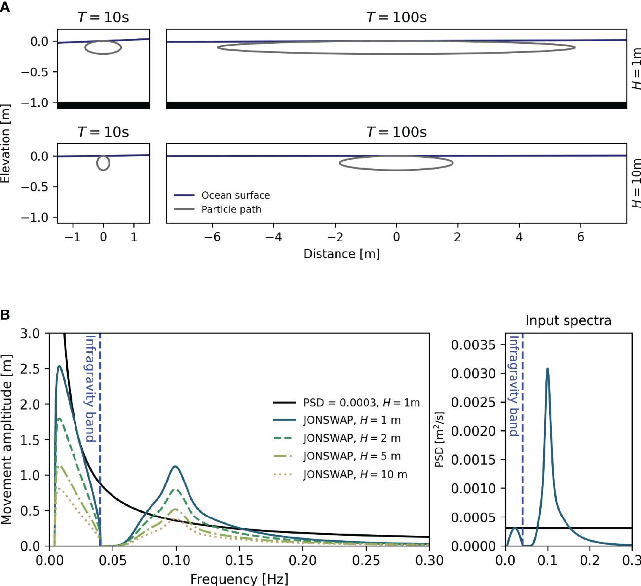
Figure 1 Fluid particle movement associated with a single wave component: (A) Pathlines for one period of a monochromatic wave with 0.1 m amplitude. Particle trajectories are found by solving Equation (2) with RK4. Left panels: a 10-second wave with amplitude for depth H = 1m and H = 10m. Right: a 100-second wave with the same amplitude and for the same two depths. It is apparent that the infragravity wave induces a much larger extent of horizontal movement. (B) Horizontal extent of particular orbit based on analytical solutions of the movement of the particle in a surface wave of a single frequency. The black curve in the left panel shows the horizontal movement associated with different wave components with equal amplitude a = 0.025m. The remaining curves show the maximum horizontal transport due to linear waves with amplitudes chosen from a JONSWAP spectrum with H_s = 0.1m and T_m = 10s, with an added infragravity component with 10% of the peak energy, and with varying depths. The right panel shows a representation of the power spectra for the case of a single wave (black line) and for the case of a JONSWAP spectrum with additional infragravity component (blue curve).

Using linear wave theory allows adding an arbitrary number of wave components in the form

$\begin{array}{ll}{\eta }_i(x,t)=A_i\text{ cos}(k_{i}x-{\omega }_{i}t+{\varphi }_i),& (5)\end{array}$

where the amplitude $A_i$ is Rayleigh distributed and the phase ϕ is uniformly distributed. The free surface is then written as a superposition $\eta (x,t)={\sum }_i{\eta }_i$ and the fluid velocity at the free surface is given by

$\begin{array}{ll}u(x,z,t)={\displaystyle \sum _i}{\omega }_i{A}_i\frac{\text{cosh}(k_i(H+z))}{\text{sinh}(k_{i}H)}\text{cos }(k_{i}x-{\omega }_{i}t+{\varphi }_i)& (6)\end{array}$

and

$\begin{array}{ll}v(x,z,t)={\displaystyle \sum _i}{\omega }_i{A}_i\frac{\text{sinh} (k_i(H+z))}{\text{sinh} (k_{i}H)}\text{sin }(k_{i}x-{\omega }_{i}t+{\varphi }_i).& (7)\end{array}$

The movement of a fluid particle can then be described by a coupled system of differential equations similar to (2) as

$\begin{array}{ll}\begin{array}{l}\frac{d\xi }{dt}=u(\xi ,\zeta ,t),\frac{d\zeta }{dt}=v(\xi ,\zeta ,t).\hfill \end{array}& (8)\end{array}$

Since the expressions for u and v are known explicitly, these equations can be solved with a standard numerical solver, such as a Runge-Kutta scheme. Instead of assuming that the velocity of the particle is close to that near the original center, we compute the particle paths directly which is feasible as long as the expressions for u and v are known in closed form [for a similar process applied to cnoidal-wave solutions, see (Borluk and Kalisch, 2012)].

Modelling the waves with Equations (5–7) and following the particle for 1800s with a time discretization of 0.25s, using the classical four-stage Runge-Kutta scheme to evolve (Equation 8) in time, and removing the linear Stokes drift, we get the results from Figure 2. Notice here that the position of the tracer is dominated by the components in the infragravity spectrum to a larger degree than predicted by the analytical case, while the amplitudes and the velocity are reminiscent of the input spectrum. Together with the analytical results, this shows that IG waves have a much larger influence on particle transport and dominate that of higher frequency waves, although they carry only a small part of the total energy of the wave field.

Figure 2

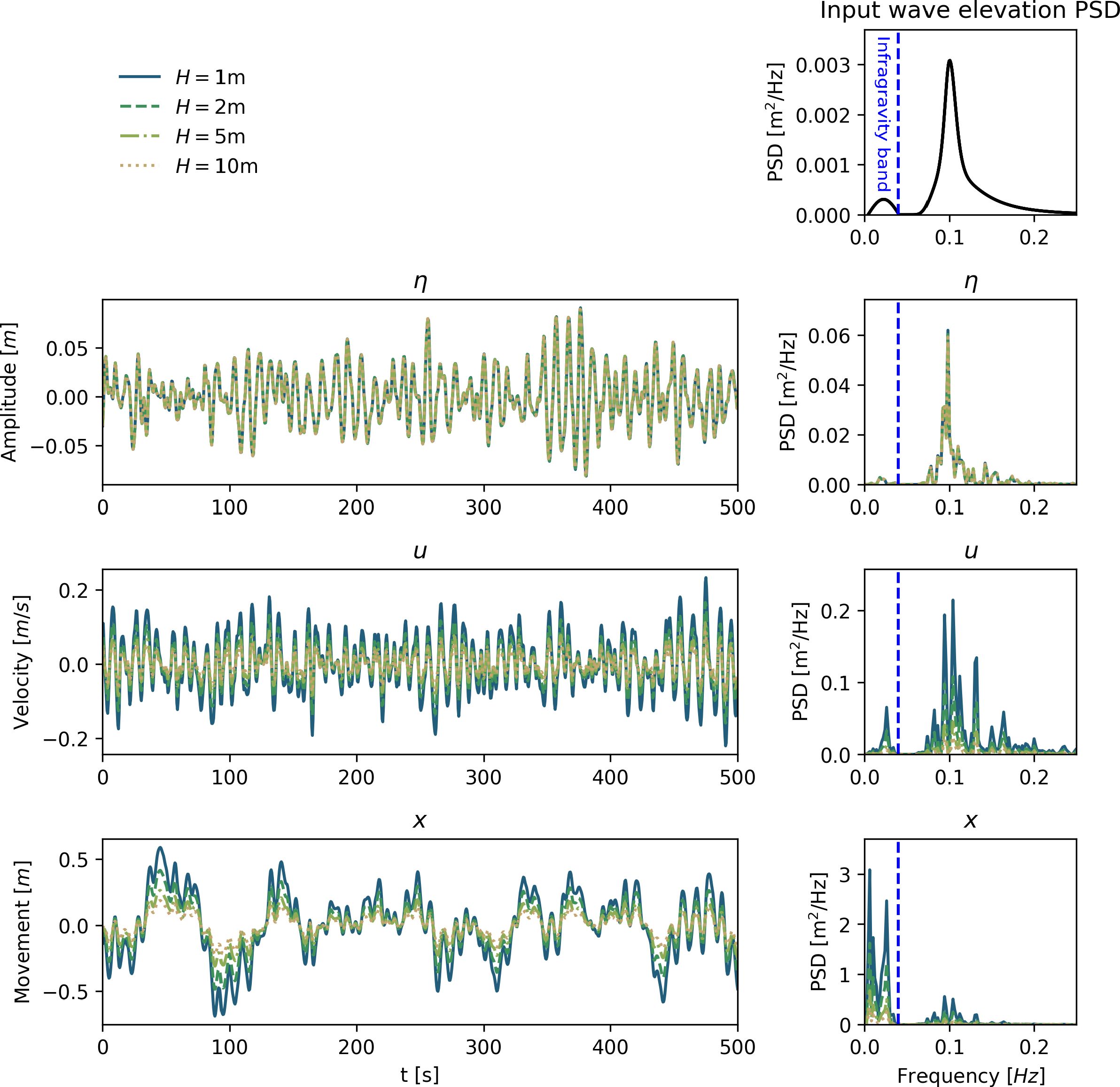
Figure 2 Experimental results from following a fluid particle moved by a superposition of waves. Top: Amplitudes of waves encountered by the particle. Middle: Velocity experienced by the particle. Bottom: Position of particle over time. Left: Time series of values. Right: Power spectral density of the time series. Colors and line-styles indicate corresponding to water depths: whole 1m, dashed 2m, dash-dot 5m, dotted 10m. For the computations shown in this Figure, 500 wave components with frequencies between 0.004Hz and 0.5Hz were used.

3 Nonlinear model

The next objective is to show that the results detailed above also hold for realistic conditions in the nearshore. To this end, we utilize BOSZ, a phase-resolving nearshore wave model based on the Nwogu equations (Roeber et al., 2010), which has been shown to yield accurate results in various situations. In particular, the model has been compared to both laboratory results (Wong et al., 2019), data from field campaigns (Roeber and Bricker, 2015) and with other models (Lynett et al., 2017). The model allows evaluation of wave-driven currents and tracking of particles.

The model is driven by imposing a sea state from a JONSWAP spectrum near the left boundary. The sea state is the same as in the earlier tests, but without the infragravity component (see Figure 3 upper right panel). In the present case, we first aim to observe IG wave generation due to nonlinear interactions in the governing equations.

Figure 3

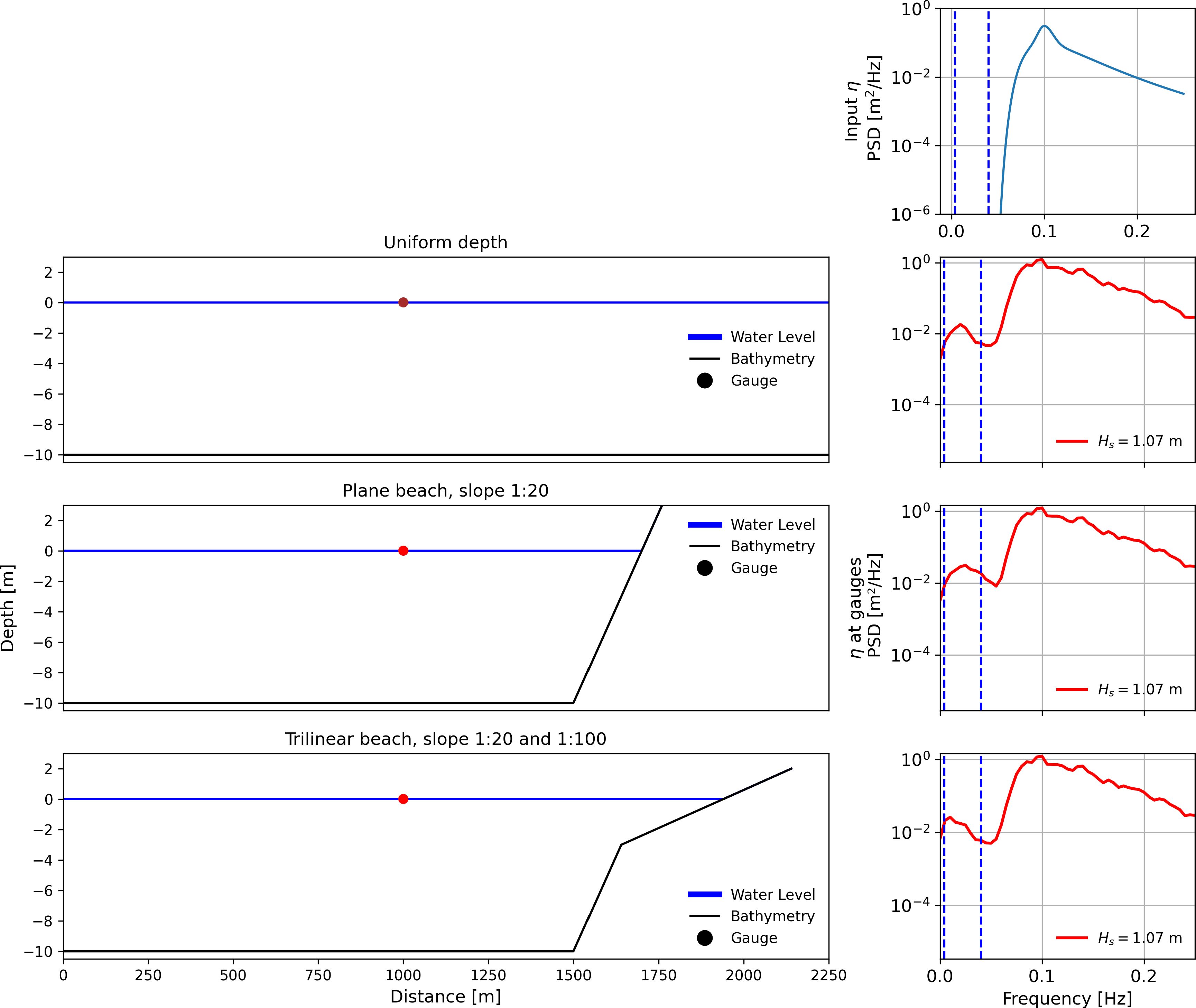
Figure 3 Comparison of infragravity wave generation from BOSZ. Upper right: the input JONSWAP spectrum to the model with H_s = 1m and T_p = 10s. Notice the lack of IG wave components in the input. Second row: A flat beach is simulated, and bound IG waves are generated as expected given the theory in (Longuet-Higgins and Stewart, 1962). Third and fourth row: with the inclusion of a beach where waves can break the IG band is increasingly significant. This is likely due to free IG waves generated in shallow water around the break point (Symonds et al., 1982; Baldock, 2012).

To verify that BOSZ can model IG-generation a computation is run for 3 hours with a 1 hour ramping time for 3 different bathymetry configurations. The wave’s free surface elevation is recorded at 1 Hz at a virtual gauge in form of a time series, from which the power spectral density is calculated. In Figure 3 one can see the bathymetries and corresponding power spectral densities (PSD). In the flat beach case both ends of the domain are padded with a sponge layer so that no reflection takes place. Thus IG wave components that are visible in the spectrum must be bound IG waves as described in (Longuet-Higgins and Stewart, 1962). For the other two bathymetries, a plane beach and a trilinear beach, the IG-band is more pronounced by a factor of 2 to 4 (see Table 1 for an overview of the bathymetries). This is likely due to free IG waves generated around the limit of the surf zone by the break point and shallow water mechanisms outlined in (Symonds et al., 1982; Baldock, 2012). In fact, applying a band-pass filter isolating the IG-wave frequencies between f = 0.004 and f = 0.04 Hz, reveals a correlation of 0.99 between the free surface and the horizontal velocity in the case of a flat bathymetry, indicating that IG waves are traveling in the direction of increasing values of x. On the other hand the correlation in the two cases with the sloping beach is 0.16 and −0.15, indicating IG waves traveling in both directions. The finding that free waves dominate vis-a-vis bound IG waves in the cases with the beach is also in line with the measurements reported on in (Smit et al., 2018).

Table 1

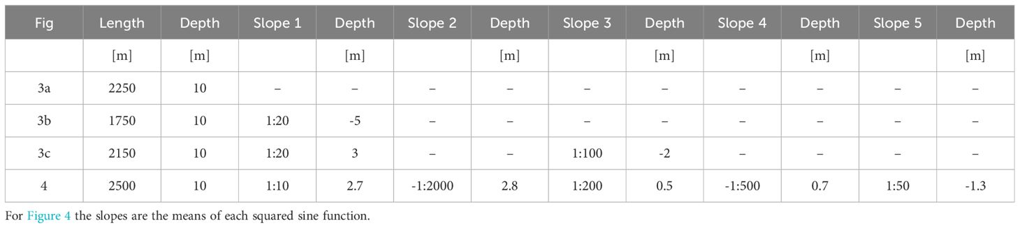
Table 1 Bathymetries used in BOSZ.

The bathymetry of the applied test of movement can be seen in the top panel of Figure 4 and in the last row in Table 1, with the locations of three measurement points (gauges) and the corresponding tracked drifters marked. The numerical domain is one-dimensional with a spatial resolution of DX = 2m. This bathymetry features a simple but realistic concept that allows us to observe the effect of IG waves on wave-induced particle transport.

Figure 4

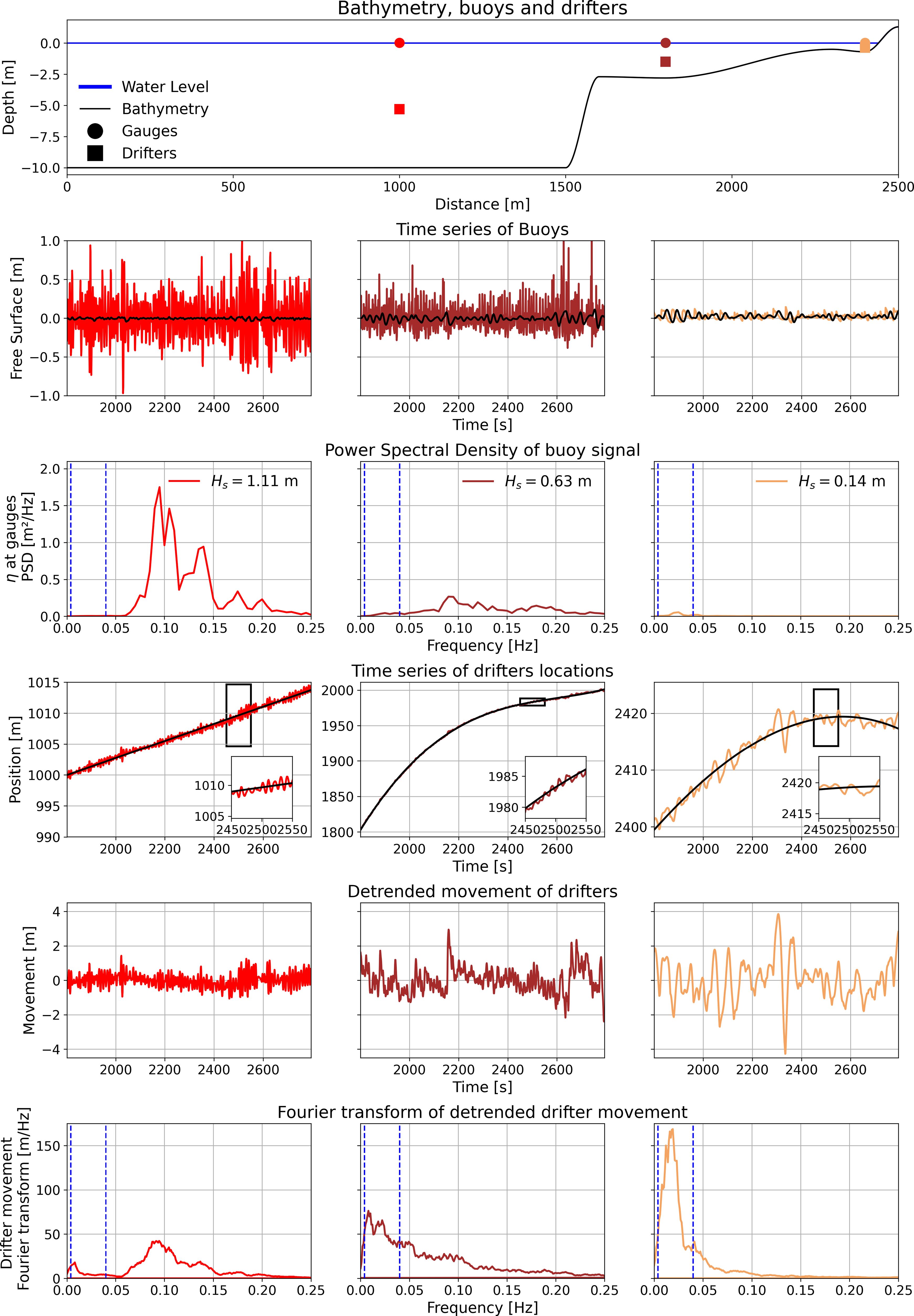
Figure 4 Numerical results for particle tracer movements. Row 1: Bathymetry and locations. Row 2: The time series of the wave elevation at the gauges. The colors and column correspond to the locations in the top plot, and the black curves are the IG-signal. Row 3: PSD of the wave elevation at the gauges. Row 4: Raw time series of the drifters location (color) together with the regression line (black). Row 5: Time series of the movement about the regression line. Row 6: PSD of the movement of the particles after the Stokes drift has been removed.

The model is run for 3600 seconds of which the first 1800 seconds are dedicated to the full development of the sea state before the fluid particles are introduced, after which they are sampled every 1 second. This yields a fundamental frequency of $f_0=\frac{1}{T}\approx 0.001$Hz and Nyquist frequency of f_max = 0.5 Hz.

Results of an in-depth time series analysis are shown in Figure 4. In the panels in row 2, the total signal as well as the low-pass filtered data recorded at the gauges is plotted. Combining this with the PSD as seen in row 3, one can see in the left column that the JONSWAP spectrum has been correctly generated by the wavemaker, but with some extra energy in the frequency band at 0.2Hz. This appears to be the result of reflected waves twice the frequency of the original JONSWAP peak. In the middle column the waves have travelled over the 1:10 slope, so that the water depth is now 2.5 meters, as opposed to 10 meters in the left column. It can be seen in the middle plot of row 3 that energy from the ordinary gravity wave spectrum has almost vanished due to bathymetry-driven wave breaking while energy starts to appear in the IG-band. Continuing on to the rightmost gauge on a now much milder slope in 1 meter depth these processes continue and the free surface is now dominated by waves in the IG band.

In row 4 the position of the three numerical drifters over time is shown. Since the numerical drifters move in the direction of the waves due to Stokes drift, it is necessary to detrend their time series signal around a moving mean position as shown in row 4 of Figure 4. For the drifter in 10 meters depth, the Stokes drift as defined in Equation 4 is constant due to the flat bathymetry, so that a first-order linear regression can be used to remove the Stokes drift from the observed drifter path. For the drifters in the shallower locations, subtracting the Stokes drift is not as straightforward. As the numerical drifters move to shallower water, the wave field and hence Stokes drift change yielding a non-constant drift, which makes a linear curve fit problematic. In such cases, a 3rd and 4th-order polynomial provided a much better fit as indicated by the black line in the middle and right column in row 4. The movement about the changing mean position for the three drifters can be seen in row 5 in Figure 4. Lastly, the Fourier transformation of this signal was taken resulting in the plots of row 6. Comparing row 3 and 6 shows the importance of the IG band on the particle movement. In the left column it is impossible, on a linear scale, to see the component of the IG band in the PSD. Nevertheless, as observed in the row 6, the IG band still has a significant influence on the movement of the drifter. For the middle row it is possible to notice the PSD component in the IG band, but it is still small compared to the size of the ordinary gravity waves. However, the particle movement is dominated by the IG wave component. Lastly, as shown in the right column of plots concerning the drifter very close to shore, the horizontal movement is almost entirely controlled by waves in the IG band. Comparing the right column with the middle and left columns, it is clear that the increased energy associated with IG waves yields a much larger movement even though the wave field is much smaller.

4 Conclusion

In the present work, the importance of IG waves on particle motion in the nearshore area has been considered in a two-dimensional setting, i.e. along a shore-normal transect. In this simplified situation, a direct link between the presence of IG waves and the main cross-shore fluid particle movement has been explored. While it is generally accepted that infragravity-wave components correlate with perturbations in the shorter-wave velocity and with horizontal velocities (see (Tissier et al., 2015) for example), the present study provides a fundamental explanation using linear wave theory and a quantification of the cross-shore motion as a function of the wave amplitude both in the linear and nonlinear case.

The study highlights what is essentially evident from linear wave theory, namely the dependence of the fluid particle excursion under waves on wave amplitude and period. It is shown in a simple yet realistic way that the horizontal motion of fluid particles in shallow water is mostly controlled by underlying IG waves, nearly independent of their amplitude, and that usual gravity waves are only of secondary importance.

This transport is essentially oscillatory in nature, i.e. it describes a back-and-forth motion of the fluid particles. This is in contrast to the Stokes drift of gravity waves that is always acting in the direction of wave propagation. The IG wave-induced motion is very large in proportion to the IG wave amplitude. In fact, even an IG wave with a tiny amplitude can lead to very large back-and-forth motions in the fluid. In the non-linear case this ratio approaches quickly 1/100. The phenomenon essentially applies in the same way to a single wave component or a spectrum, and it also occurs in a similar fashion in nonlinear waves as shown by a Boussinesq-type model. The principles also hold consistently for non-uniform seabeds.

In nature, the behavior of IG waves depends at various levels on other factors such as the direction of the incoming wave field (Herbers et al., 1995a), local beach morphology (Bryan et al., 1998), or the tide stage (Melito et al., 2022), to name only a few. Obviously, three-dimensional dynamics will generally affect the IG wave signal, in particular in connection with the appearance of edge waves (Herbers et al., 1995b), IG wave reflection (Sheremet et al., 2002), as well as eventual propagation off-shore and refraction at the shelf break (Smit et al., 2018).

As already mentioned, IG waves are connected to a wide range of nearshore processes, and the results in this paper are in line with recent observations of horizontal movement of freshwater plumes (Flores et al., 2022) and also with wave-by-wave motions of tracer particles in the nearshore (Bjørnestad et al., 2021).

While the objective of this study is not to identify the processes responsible for sediment transport, this work validates and quantifies the findings by (Aagaard and Greenwood, 2008) about the underlying physics of IG wave-driven motion of sediment. In reality, the mechanism showcased in this article will rarely be the only controlling process and may not always be easily detectable in a three-dimensional setting. However, as shallow water regimes naturally tend to exhibit waves in the IG band due to non-linear bathymetric effects, the results provided here suggest that the horizontal motion induced by IG waves always plays a key role.

Data availability statement

The original contributions presented in the study are included in the article/supplementary material. Further inquiries can be directed to the corresponding author.

Author contributions

AB: Conceptualization, Formal analysis, Investigation, Methodology, Software, Visualization, Writing – original draft, Writing – review & editing. HK: Conceptualization, Formal analysis, Funding acquisition, Investigation, Methodology, Supervision, Writing – original draft, Writing – review & editing. VR: Conceptualization, Formal analysis, Methodology, Resources, Software, Supervision, Validation, Writing – original draft, Writing – review & editing.

Funding

The author(s) declare financial support was received for the research, authorship, and/or publication of this article. HK acknowledges support from Bergen Universitetsfond. VR acknowledges financial support from the I-SITE program Energy & Environment Solutions (E2S), the Communauté d’Agglomération Pays Basque (CAPB), and the Communauté Région Nouvelle Aquitaine (CRNA) for the E2S chair position HPC-Waves.

Acknowledgments

The authors would like to thank Alexander Horner-Devine for providing some inspiration for undertaking the present study. The authors would like to thank Dr. Tomohiro Suzuki for providing the raw data of the laboratory experiment referenced in Suzuki et al. (2017).

Conflict of interest

The authors declare that the research was conducted in the absence of any commercial or financial relationships that could be construed as a potential conflict of interest.

Publisher’s note

All claims expressed in this article are solely those of the authors and do not necessarily represent those of their affiliated organizations, or those of the publisher, the editors and the reviewers. Any product that may be evaluated in this article, or claim that may be made by its manufacturer, is not guaranteed or endorsed by the publisher.

References

Aagaard T., Greenwood B. (2008). Infragravity wave contribution to surf zone sediment transport—the role of advection. Mar. Geology 251, 1–14. doi: 10.1016/j.margeo.2008.01.017

CrossRef Full Text | Google Scholar

Baldock T. (2012). Dissipation of incident forced long waves in the surf zone — implications for the concept of “bound” wave release at short wave breaking. Coast. Eng. 60, 276–285. doi: 10.1016/j.coastaleng.2011.11.002

CrossRef Full Text | Google Scholar

Bertin X., De Bakker A., Van Dongeren A., Coco G., Andre G., Ardhuin F., et al. (2018). Infragravity waves: From driving mechanisms to impacts. Earth-Science Rev. 177, 774–799. doi: 10.1016/j.earscirev.2018.01.002

CrossRef Full Text | Google Scholar

Bjørnestad M., Buckley M., Kalisch H., Streßer M., Horstmann J., Frøysa H. G., et al. (2021). Lagrangian measurements of orbital velocities in the surf zone. Geophysical Res. Lett. 48, e2021GL095722. doi: 10.1029/2021GL095722

CrossRef Full Text | Google Scholar

Borluk H., Kalisch H. (2012). Particle dynamics in the KdV approximation. Wave Motion 49, 691–709. doi: 10.1016/j.wavemoti.2012.04.007

CrossRef Full Text | Google Scholar

Bryan K., Howd P., Bowen A. (1998). Field observations of bar-trapped edge waves. J. Geophysical Research: Oceans 103, 1285–1305. doi: 10.1029/97JC02938

CrossRef Full Text | Google Scholar

Castelle B., Scott T., Brander R., McCarroll R. (2016). Rip current types, circulation and hazard. Earth-Science Rev. 163, 1–21. doi: 10.1016/j.earscirev.2016.09.008

CrossRef Full Text | Google Scholar

Davidson-Arnott R., Bauer B., Houser C. (2019). Introduction to coastal processes and geomorphology. (Cambridge: Cambridge University Press).

Google Scholar

Debnath L. (1994). Nonlinear water waves. (San Diego: Academic Press).

Google Scholar

Flores R. P., Williams M. E., Horner-Devine A. R. (2022). River plume modulation by infragravity wave forcing. Geophysical Res. Lett. Academic Press: San Diego 49, e2021GL097467.

Google Scholar

Hasselmann K., Barnett T. P., Bouws E., Carlson H., Cartwright D. E., Enke K., et al. (1973). Measurements of wind-wave growth and swell decay during the joint north sea wave project (jonswap). Ergaenzungsheft zur Deutschen Hydrographischen Zeitschrift Reihe A. 12, 7–93

Google Scholar

Herbers T., Elgar S., Guza R. (1994). Infragravity-frequency (0.005–0.05 hz) motions on the shelf. part i: Forced waves. J. Phys. Oceanography 24, 917–927. doi: 10.1175/1520-0485(1994)024<0917:IFHMOT>2.0.CO;2

CrossRef Full Text | Google Scholar

Herbers T., Elgar S., Guza R. (1995a). Generation and propagation of infragravity waves. J. Geophysical Research: Oceans 100, 24863–24872. doi: 10.1029/95JC02680

CrossRef Full Text | Google Scholar

Herbers T., Elgar S., Guza R., O’Reilly W. (1995b). Infragravity-frequency (0.005–0.05 hz) motions on the shelf. part ii: Free waves. J. Phys. Oceanography 25, 1063–1079. doi: 10.1175/1520-0485(1995)025<1063:IFHMOT>2.0.CO;2

CrossRef Full Text | Google Scholar

Holthuijsen L. H. (2010). Waves in oceanic and coastal waters. (Cambridge: Cambridge university press).

Google Scholar

Kalisch H., Lagona F., Roeber V. (2024). Sudden wave flooding on steep rock shores: a clear but hidden danger. Natural Hazards 120, 3105–3125. doi: 10.1007/s11069-023-06319-w

CrossRef Full Text | Google Scholar

Kenyon K. E. (1969). Stokes drift for random gravity waves. J. Geophysical Res. 74, 6991–6994. doi: 10.1029/JC074i028p06991

CrossRef Full Text | Google Scholar

Kinsman B. (1984). Wind waves: their generation and propagation on the ocean surface. (New York: Courier Corporation).

Google Scholar

Kundu P. K., Cohen I. M. (2015). Fluid mechanics. (San Diego: Academic Press).

Google Scholar

Lamb H. (1924). Hydrodynamics. (Cambridge: University Press).

Google Scholar

Longuet-Higgins M. S. (1984). Statistical properties of wave groups in a random sea state. Philosophical Transactions of the Royal Society of London. Ser. A Math. Phys. Sci. 312, 219–250.

Google Scholar

Longuet-Higgins M. S., Stewart R. W. (1962). Radiation stress and mass transport in gravity waves, with application to ‘surf beats’. J. Fluid Mechanics 13, 481–504. doi: 10.1017/S0022112062000877

CrossRef Full Text | Google Scholar

Lynett P. J., Gately K., Wilson R., Montoya L., Arcas D., Aytore B., et al. (2017). Inter-model analysis of tsunami-induced coastal currents. Ocean Model. 114, 14–32. doi: 10.1016/j.ocemod.2017.04.003

CrossRef Full Text | Google Scholar

McWilliams J. C., Restrepo J. M. (1999). The wave-driven ocean circulation. J. Phys. Oceanography 29, 2523–2540. doi: 10.1175/1520-0485(1999)029<2523:TWDOC>2.0.CO;2

CrossRef Full Text | Google Scholar

Melito L., Parlagreco L., Devoti S., Brocchini M. (2022). Wave-and tide-induced infragravity dynamics at an intermediate-to-dissipative microtidal beach. J. Geophysical Research: Oceans 127, e2021JC017980.

Google Scholar

Mendes D., Fortunato A. B., Bertin X., Martins K., Lavaud L., Nobre Silva A., et al. (2020). Importance of infragravity waves in a wave-dominated inlet under storm conditions. Continental Shelf Res. 192, 104026. doi: 10.1016/j.csr.2019.104026

CrossRef Full Text | Google Scholar

Munk W. (1949). Surf beats Vol. 30. (EOS, Transactions American Geophysical Union), 849–854.

Google Scholar

Munk W. H. (1951). Origin and generation of waves. (La Jolla: Tech. rep., Scripps Institution of Oceanography La Jolla Calif).

Google Scholar

Péquignet A.-C. N., Becker J. M., Merrifield M. A. (2014). Energy transfer between wind waves and low-frequency oscillations on a fringing reef, Ipan, Guam. J. Geophysical Research: Oceans 119, 6709–6724. doi: 10.1002/2014JC010179

CrossRef Full Text | Google Scholar

Pierson W. J. Jr., Moskowitz L. (1964). A proposed spectral form for fully developed wind seas based on the similarity theory of sa kitaigorodskii. J. geophysical Res. 69, 5181–5190. doi: 10.1029/JZ069i024p05181

CrossRef Full Text | Google Scholar

Roeber V., Bricker J. D. (2015). Destructive tsunami-like wave generated by surf beat over a coral reef during typhoon haiyan. Nat. Commun. 6, 7854. doi: 10.1038/ncomms8854

PubMed Abstract | CrossRef Full Text | Google Scholar

Roeber V., Cheung K. F., Kobayashi M. H. (2010). Shock-capturing boussinesq-type model for nearshore wave processes. Coast. Eng. 57, 407–423. doi: 10.1016/j.coastaleng.2009.11.007

CrossRef Full Text | Google Scholar

Russell P. E. (1993). Mechanisms for beach erosion during storms. Continental Shelf Res. 13, 1243–1265. doi: 10.1016/0278-4343(93)90051-X

CrossRef Full Text | Google Scholar

Sheremet A., Guza R., Herbers T. (2002). Observations of nearshore infragravity waves: Seaward and shoreward propagating components. J. Geophysical Research: Oceans 107, 10–11. doi: 10.1029/2001JC000970

CrossRef Full Text | Google Scholar

Smit P., Janssen T., Herbers T., Taira T., Romanowicz B. (2018). Infragravity wave radiation across the shelf break. J. Geophysical Research: Oceans 123, 4483–4490. doi: 10.1029/2018JC013986

CrossRef Full Text | Google Scholar

Stokes G. G. (1847). On the theory of oscillatory waves. Trans. Cam. Philos. Soc 8, 441–455.

Google Scholar

Suzuki T., Altomare C., Veale W., Verwaest T., Trouw K., Troch P., et al. (2017). Efficient and robust wave overtopping estimation for impermeable coastal structures in shallow foreshores using swash. Coast. Eng. 122, 108–123. doi: 10.1016/j.coastaleng.2017.01.009

CrossRef Full Text | Google Scholar

Svendsen I. A. (1984). Wave heights and set-up in a surf zone. Coast. Eng. 8, 303–329. doi: 10.1016/0378-3839(84)90028-0

CrossRef Full Text | Google Scholar

Symonds G., Huntley D. A., Bowen A. J. (1982). Two-dimensional surf beat: Long wave generation by a time-varying breakpoint. J. Geophysical Research: Oceans 87, 492–498. doi: 10.1029/JC087iC01p00492

CrossRef Full Text | Google Scholar

Thompson W. C., Nelson A. R., Sedivy D. G. (1984). Wave group anatomy of ocean wave spectra. Coastal Engineering Proceedings. 1 (19), 45. doi: 10.9753/icce.v19.45

CrossRef Full Text | Google Scholar

Tissier M., Bonneton P., Michallet H., Ruessink B. (2015). Infragravity-wave modulation of short-wave celerity in the surf zone. J. Geophysical Research: Oceans 120, 6799–6814. doi: 10.1002/2015JC010708

CrossRef Full Text | Google Scholar

Tucker M. (1950). Surf beats: Sea waves of 1 to 5 min. period. Proc. R. Soc. London. Ser. A. Math. Phys. Sci. 202, 565–573.

Google Scholar

van Thiel de Vries J., van Gent M., Walstra D., Reniers A. (2008). Analysis of dune erosion processes in large-scale flume experiments. Coast. Eng. 55, 1028–1040. doi: 10.1016/j.coastaleng.2008.04.004

CrossRef Full Text | Google Scholar

Wong W.-Y., Bjørnestad M., Lin C., Kao M.-J., Kalisch H., Guyenne P., et al. (2019). Internal flow properties in a capillary bore. Phys. Fluids 31. doi: 10.1063/1.5124038

CrossRef Full Text | Google Scholar

Appendix: validation of BOSZ

For validation of the BOSZ model’s ability in replicating the evolution of the wave field and generation of IG-waves across a varying bathymetry we include the replication of the results from the laboratory test described in Suzuki et al. (2017). The test is useful for validation of the numerical model’s ability in handling the process of wave shoaling and transformation of energy levels across an entire spectrum including the breaking process with subsequent transfer and dissipation of energy. This test consists of a 1D channel with a 1:35 slope. The wave field is based on a Pierson-Moskowitz spectrum. The boundary condition in the model uses a free surface times series initially recorded at an offshore wave gauge during the experiment.

The test was run with a grid of Δx = 0.01 m, the results of which can be seen in Figure A1. Significant for this article, BOSZ is able to capture the evolution of the wave field from generation to very small depths. Further, it is evident that it manages to account for the shift of energy to higher frequencies in the shoaling process and the dissipation in the wave breaking process and the subsequent transfer to lower frequencies in the IG band. For more details, please consult Kalisch et al. (2024).

Figure A1

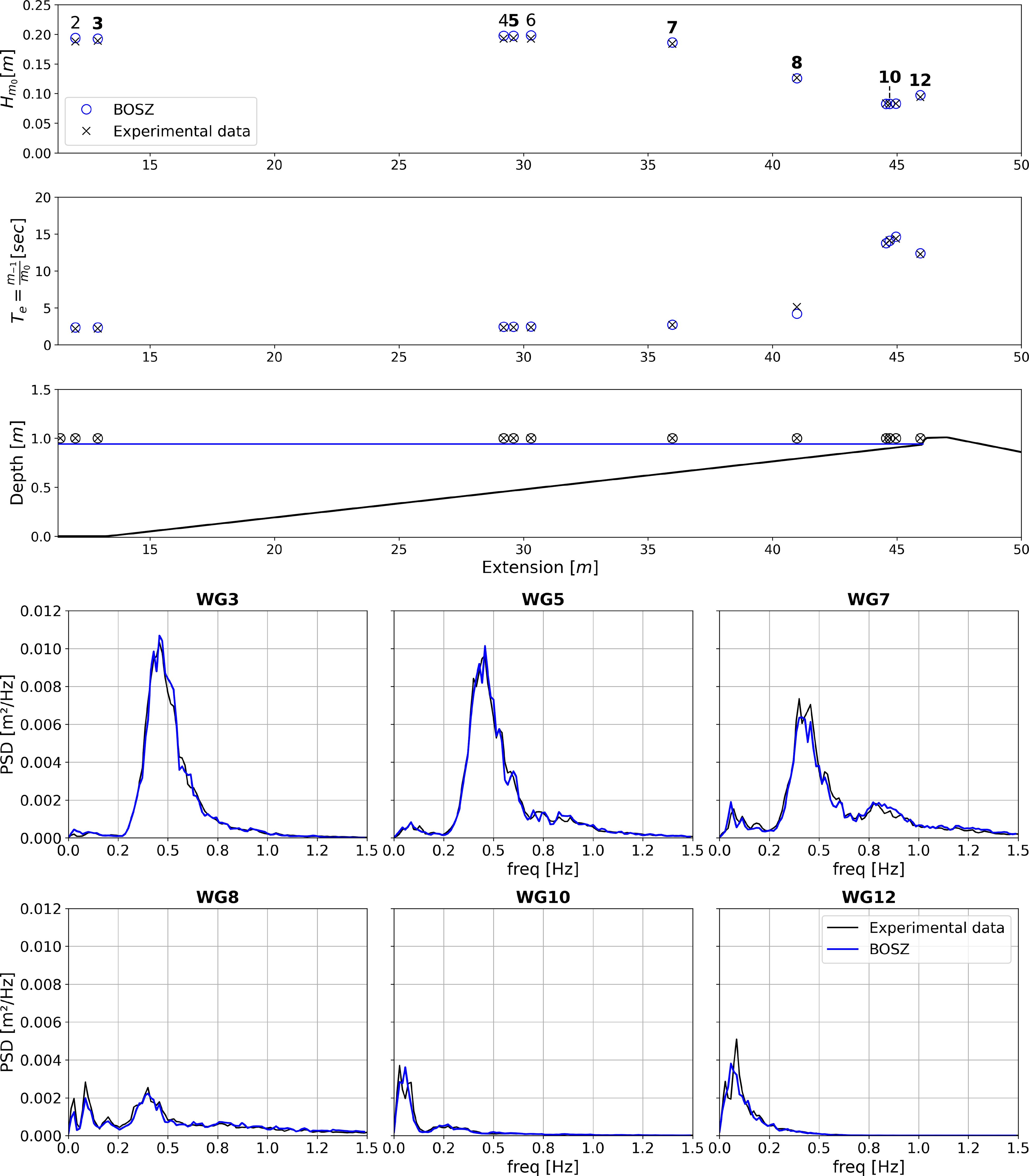
Figure A1 Comparison between the numerical solution of BOSZ and the laboratory data from Suzuki et al. (2017). Row 1 shows the comparison of significant wave height at multiple gauge locations, and row 2 to the corresponding energy period. Row 3 shows the locations of the gauges in the wave channel. The last two rows show the entire spectrum for 6 of the locations.