Evolution of 3-D chlorophyll in the northwestern Pacific Ocean using a Gaussian-activation deep neural network model

1 Introduction

Marine phytoplankton provides nearly half of the global primary production (Behrenfeld, 2001) and plays critical roles in regulating ecosystem and carbon cycle in the global ocean (Gregg et al., 2003; Anderson et al., 2021). Popularly, Chlorophyll-a concentration (Chl-a) has served as an index in estimating phytoplankton biomass, primary production, and the trophic condition in the ocean (Volpe et al., 2012; Colella et al., 2016; Hammond et al., 2020). So far, satellite remote sensing is a major source of marine Chl-a data, meanwhile these data are limited within the surface ocean that contains generally less than 20% of the euphotic depths for phytoplankton photosynthesis process (Gordon and McCluney, 1975; Matthes et al., 2023), thus unable to reveal subsurface chlorophyll maxima (SCMs) beneath the surface mixed layer. The SCMs are a ubiquitous and prominent characteristic in both coastal seas and open oceans, commonly believed to form in specific regions of the water column where opposing gradients of light and nutrients, coupled with turbulent mixing, create conditions conducive to optimal phytoplankton growth (Cullen and Eppley, 1981; Letelier et al., 2004; Beckmann and Hense, 2007; Cullen, 2015; Cornec et al., 2021). The SCMs significantly contribute to primary production, highlighting their crucial role in marine ecosystems (Fennel and Boss, 2003; Gong et al., 2015, 2017). Therefore, the mis-detection of SCMs by satellite leads to limitation and also significant errors in estimating temporal evolution of 3-D structure in the Chl-a production, with regional errors even to 120% (Piatt et al., 1989; Fernand et al., 2013; Bouman et al., 2020).

Since the 1980s, how to retrieval Chl-a vertical distributions from surface-ocean data has been a subject of considerable attention since the 1980s (Morel and Berthon, 1989). Statistical extrapolation method is employed to derive vertical profile of Chl-a, commonly by incorporating satellite-derived data (Morel and Berthon, 1989; Richardson et al., 2003; Uitz et al., 2006). This approach involves partitioning oceanic waters into trophic categories based on their surface Chl-a values, ranging mainly from 0.01 mg m^-3 to over 10 mg m^-3. The mean vertical Chl-a profile in each category is then computed using generalized Gaussian functions (Platt et al., 1988; Gong et al., 2015). However, this method fails adequately describing the shape of Chl-a profiles in various areas and on daily timescales. In parallel, numerical models simulating gridded vertical Chl-a profiles show large discrepancies, likely attributed to inconsistent modeling parameters strategy and various grid-mesh resolutions (Varela et al., 1992; Moeller et al., 2019; Masuda et al., 2021; Shu et al., 2022).

Recently, more and more artificial intelligence technology is employed to reconstruct vertical structure of ocean Chl-a on the basis of satellite remote sensing data. For instance, Sammartino et al. (2018) utilized an artificial neural network (ANN) model (single hidden layer) on sea surface temperature (SST) and surface Chl-a data, to infer the vertical profiles of Chl-a in the Mediterranean Sea. Similarly, also based on SST and surface-ocean Chl-a datasets, Chen et al. (2022a) and Wang et al. (2023a) analyzed SCMs in the northwestern Pacific Ocean (NWPO) using deep learning models. However, their studies commonly overlooked potential impacts of network design along ocean depths in accuracy to the results. There are some studies that utilize vertical variables as predictors. For example, Sauzède et al. (2016) utilized an ANN model to infer vertical profiles of the particulate backscattering coefficient based on surface ocean-color estimates, vertical potential densities, and mixed-layer depths. Similarly, Hu et al. (2023) employed a Random Forest (RF) method to retrieve vertical Chl-a profiles in the northern Indian Ocean, utilizing surface ocean-color estimates, vertical temperature and salinity, and mixed-layer depths as inputs. Although their studies improved the estimation accuracy of 3-D structure by incorporating vertical physical properties, they solely demonstrate the feasibility of climatology monthly vertical structure or are restricted to the time span of the input data, leaving the long-term 3-D Chl-a reconstruction problem unresolved.

The NWPO boasts one of the richest marine ecosystems (Naiman et al., 1992) with abundant and diverse fishery resources in the global ocean (Chikuni, 1986), and the atmosphere-ocean coupled system in the NWPO is closely linked to the global warming and also provides critical feedbacks (Xie et al., 2009; Kulk et al., 2020; Shi et al., 2023). A few of studies investigated the variabilities of surface Chl-a on the long-term trends in the NWPO (Hammond et al., 2020; Chen et al., 2022b; Yu et al., 2023). Significant negative trends of surface Chl-a are generally observed in the oligotrophic gyres of the NWPO during 1998–2020 (Yu et al., 2023). In the subarctic gyres of the NWPO, surface Chl-a presented an increased tendency during 1997–2020 (Chen et al., 2022b). However, given the prevailing SCMs in the NWPO (Cornec et al., 2021; Chen et al., 2022a; Wang et al., 2023a), caution is warranted when extending conclusions from surface Chl-a to water-column integrated Chl-a. Meanwhile, the lack of long-term 3-D Chl-a structure means that trends in water-column integrated Chl-a in the NWPO remain an open question.

In this study, we engaged in extrapolative prediction for long-term, gridded vertical Chl-a profiles in the NWPO using an enhanced deep neural network (DNN) model. DNN models, as a subset of deep learning, are distinguished by their multiple hidden layers compared to ANN models, which typically have a single hidden layer. They possess the capability to autonomously extract intricate features from raw data and demonstrate higher scalability in managing extensive and complex datasets (Li et al., 2020). Moreover, DNN models have been certified to exhibit superior performance in retrieving vertical bio-optical properties (e.g., Chl-a, nitrate) compared to ANN models (Chen et al., 2022a; Wang et al., 2023a, b) and RF models (Wang et al., 2023a) in the NWPO. Therefore, through the precise reconstruction of 3-D Chl-a using an enhanced DNN model, our study aims to an improved understanding of the variability of SCMs characteristics and long-term trends in depth-integrated Chl-a in the NWPO. This, in turn, aids in elucidating the regional carbon cycle and marine ecosystem dynamics, while also offering valuable insights for future projections.

This paper is organized as: Section 2 provides the detailed information on the DNN model based on a Gaussian activation function (named as Gaussian-DNN), along with the data used for model training, validation, and reconstruction, as well as the evaluation methods employed in this study. In Section 3, the trained Gaussian-DNN was validated using two independent datasets and proceeded to reconstruct long-term 3-D Chl-a structures in the NWPO. Furthermore, based on the reconstruction, Section 3 analyzed the spatiotemporal variations of SCM characteristics and long-term trends in depth-integrated Chl-a in water columns. Section 4 includes a sensitivity test for input variables and a discussion on the importance of each input in the developed DNN model for controlling the spatiotemporal distribution of Chl-a in the NWPO, along with a discussion on the uncertainties of our DNN model. In the end, a summary of our key findings are illustrated in Section 5.

2 Data and methods

2.1 Data processing

2.1.1 Training data from Biogeochemical-Argo dataset

The BGC-Argo program, a pioneering initiative utilizing profiling floats for ocean-wide and distributed ocean monitoring (Bittig et al., 2019), collects 3-D ocean variables including temperature, salinity and Chl-a (https://biogeochemical-argo.org/). Field data utilized to train the DNN model were obtained from 35 BGC-Argo profiling floats in the NWPO region of 123 - 180°E, 12 - 54°N, as shown in Figure 1A. In total, BGC-Argo floats provide 3941 vertical Chl-a profiles, spanning all seasons from July 2017 to October 2022. In the data preparation stage, we first corrected the overestimation of BGC-Argo Chl-a by implementing a factor-two adjustment, as recommended by Cornec et al. (2021). Subsequently, we identified and removed 9 vertical Chl-a profiles with sea surface values exceeding 6.5 mg m^-3, following the criteria established by Venrick et al. (1987). Additionally, upon visual inspection, 173 profiles were flagged as abnormal and excluded from the dataset. Among these, 123 profiles exhibited consistent concentrations with minor fluctuations within the surface 20 m, while the remaining 50 profiles displayed anomalously high values below a depth of 250 meters, identified using the 3σ rule. Furthermore, we applied the Savitzky-Golay filtering method to refine the remaining profiles (Press and Teukolsky, 1990). Ultimately, a dataset comprising 3,759 vertical Chl-a profiles, along with paired temperature and salinity data, was retained for training the Gaussian-DNN model. Following the assumptions of Cornec et al. (2021) about phytoplankton living habitat, we applied our model for the ocean of 0–300 m.

Figure 1

Figure 1 (A) Locations and measurement months of 35 BGC-Argo buoys in the Northwest Pacific Ocean. (B) Ship measured sites during cruises RF and KS from Japan Maritime Agency (JMA). Data at N-S transects of 137°E and 165°E highlighted to present the validation process.

In our analysis, based on our statistical analysis on SCMs characteristics (See Chen et al., 2022a), the 35 profiling floats of the BGC-Argo are catalogued to three boxes to represent the tropics (12–24°N), the subtropical (24–38°N) and temperate (38–54°N) gyres, respectively (Figure 1A), aiming to illustrate the variations in vertical Chl-a distribution across latitudes in the NWPO.

2.1.2 Validation data from ship measurements

To assess the robustness and generalization of the trained DNN model on datasets from different sources, the datasets of Japan Meteorological Agency (JMA) from April 2015 to March 2021 (https://www.jma.go.jp/jma/indexe.html) are obtained, as shown in Figure 1B. We retained a total of 937 profiles of Chl-a and their corresponding temperature-salinity profiles. The Chl-a data from JMA spans a range of 0 to 19.83 mg m^-3. Similar to the data processing for BGC-Argo float data, after filtering out Chl-a profiles with sea surface values greater than 6.5 mg m^-3, 924 profiles remained for deployment in the trained Gaussian-DNN model. The vertical resolution of the Chl-a data in the JMA dataset is at standard layers of 0, 5, 10, 25, 50, 75, 100, 150, 200, 250, and 300 m, and the predicted Chl-a values at these depths were output from the trained Gaussian-DNN model.

All retained measurement points were utilized for validating the Gaussian-DNN model. The choice of N-S transects at 137°E and 165°E was driven by their comprehensive tempo-spatial coverage across all seasons and multiple sub-regions, rendering them ideal for elucidating the validation process.

2.1.3 Reconstruction data from satellite and Argo

Satellite Chl-a data were obtained to reconstruct gridded vertical distribution of Chl-a in the NWPO by using the trained DNN model. Monthly Level-3 Chl-a data products from the MODIS Aqua satellite, with a standard resolution of 9 km, were collected from January 2004 to June 2022, sourced from the NASA Goddard Space Flight Center (http://oceancolor.gsfc.nasa.gov/, accessed on 13 April 2023). Subsequently, we conducted a comparative analysis between MODIS Chl-a values and those derived from BGC-Argo datasets. The results are comparable between them, although some discrepancies are noted within the domain of 0–0.2 mg m^-3 (Supplementary Figure 1). This indicates the potential effectiveness of MODIS data in complementing our Gaussian-DNN model trained with BGC-Argo data.

Within the MODIS Chl-a dataset we acquired, there is an overall missing rate of approximately 5% in the NWPO, primarily attributable to cloud cover. Spatially, the regions with high missing data rates are temperate waters (BOX3), with an average missing data rate of about 30% (Supplementary Figure 2). Following this, the subtropical area (BOX2) exhibits an average missing data rate of about 10%. Conversely, the tropical region (BOX1) shows minimal missing data. Given our focus on reconstructing the 3-D gridded Chl-a structure using surface Chl-a, we applied the Data Interpolating Empirical Orthogonal Functions (DINEOF) method to fill in the gaps of MODIS Chl-a (see Supplementary Figure 3). DINEOF is an interpolation method suitable for handling remote sensing and oceanographic data with missing values (Beckers and Rixen, 2003; Alvera-Azcárate et al., 2005; Liu and Wang, 2018, 2023). It decomposes data into spatial and temporal components using empirical orthogonal functions (EOFs) and utilizes linear combinations of orthogonal functions to estimate missing values. By selecting the most important spatial and temporal modes and employing an iterative optimization strategy to progressively refine the estimates, DINEOF is capable of producing relatively accurate interpolation results, contributing to the restoration of data integrity and accuracy.

Additionally, temperature-salinity profiles obtained from Argo profiling buoys were utilized as gridded high-resolution data, allowing the incorporation of known deep hydrographic information into the inference of gridded Chl-a vertical profiles. These temperature and salinity profiles were obtained from the global ocean Argo grid dataset (BOA-Argo), accessible through the China Argo Real-Time Data Center website (http://www.argo.org.cn/) or the Argo Program Office website (http://www.argo.ucsd.edu/). This dataset is available from January 2004 onwards, with a spatial resolution of 1°×1°. The BOA-Argo dataset was generated through Barnes successive corrections following stringent quality recontrol of real-time global ocean Argo data (Li et al., 2017). It is also available for download from the Argo Program Office website (http://www.argo.ucsd.edu/). Extensive evaluations have confirmed its robust comparability with various other Argo gridded datasets, including WOA13, Roemmich-Argo, Jamestec-Argo, EN4-Argo, and IPRC-Argo, across multiple metrics such as climatology, independent observations, mixed-layer depth, and more (Li et al., 2017). This dataset comprises 48 vertical levels between 0 and 1975 meters in depth, with intervals as follows: 5 m, 10–200 m at 10 m intervals, 220–500 m at 20 m intervals, 600–1500 m at 100 m intervals, 1750 m, and 1950 m. To retrieve the depth-resolved Chl-a profiles, we employed linear interpolation to adjust the BOA-Argo temperature-salinity profiles to a 1-meter interval within the 0–300 m depth range.

The monthly MODIS Chl-a and BOA-Argo thermohaline data were synchronized to create the input dataset for reconstructing 3-D Chl-a structures. This synchronization began in January 2004, aligning with the earliest available thermohaline data provided by the BOA-Argo dataset. Additionally, to ensure compatibility with the BOA-Argo data, the MODIS gap-free Chl-a data underwent processing to achieve a spatial resolution of 1°×1° using a bilinear interpolation method. This yielded a surface Chl-a dataset containing a total of 400,044 data points, with 109 points surpassing 6.5 mg m^-3. Given the negligible influence of relatively small percentage of high values (0.03%) on network performance and the constitution of data, we retained these 109 points. Overall, the input data used for reconstruction consisted of monthly datasets spanning from January 2004 to June 2022, characterized by a spatial resolution of 1°×1° and a vertical resolution of 1 meter.

2.2 DNN model configuration

DNN, a deep learning method characterized by multiple hidden layers in its neural network architecture, was employed in our study with 4 hidden layers (Figure 2). Compared with a conventional ANN, the use of multiple hidden layers allows DNN models to learn more efficient and compact representations of the data, leading to better scalability and performance on large-scale datasets (Li et al., 2020). Generally, operation of our DNN model involves two main steps of forward propagation and backward propagation. In the back-propagation step, our DNN model is trained with the Adam optimizer utilized gradient descent. To prevent overfitting, we additionally employed a dropout technique, strategically discarding some neurons. Through continuous iterations between these two steps, our DNN model minimizes the loss value within training procedure.

Figure 2

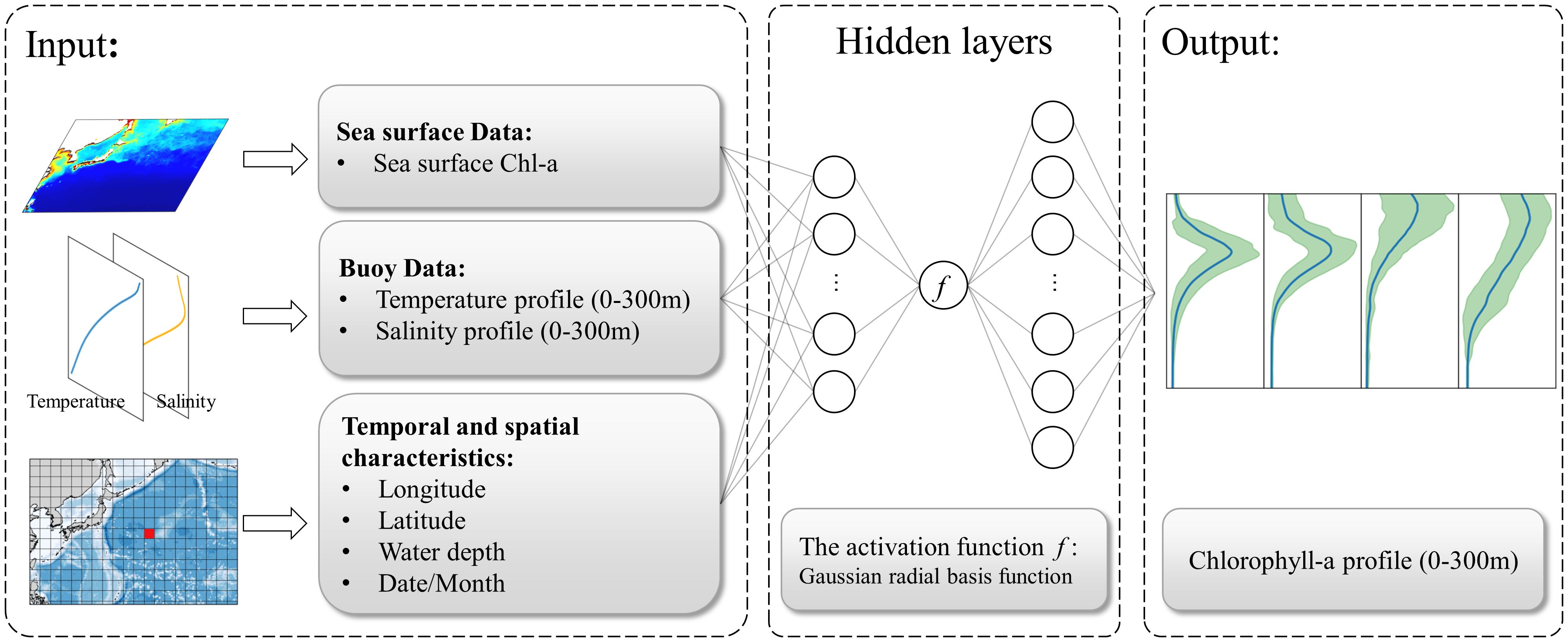
Figure 2 The structure of the enhanced Gaussian-activation deep neural network (Gaussian-DNN). The input elements for the Gaussian-DNN include sea surface Chl-a, vertical properties such as temperature and salinity, along with corresponding geographical coordinates (longitude, latitude, and water depth) and temporal information (month). The output predictor represents the vertical distribution of Chl-a concentrations with a 1 m interval within the 0–300 m water depth range.

Our DNN model employed a Gaussian radial basis function (Equation 1) as the nonlinear activation function (Figure 2).

$\begin{array}{ll}f=e^{-\pi {(X_j-b)}^2}& (1)\end{array}$

where $X_j$ is the value of the $j$^th output in the hidden layer, b is the bias term. The Gaussian radial basis function exhibits a bell-shaped curve, resembling a quadratic function for the center values of input variables (Sharma et al., 2020). Compared to conventional activation functions such as sigmoid or tanh, the Gaussian activation function has been shown to offer superior performance in solving nonlinear problems (Gundogdu et al., 2015). It is notable that Chen et al. (2022a) demonstrated that the Gaussian activation function is more effective in capturing SCMs features compared to the sigmoid activation function.

In the set-up of our DNN model, we deliberately initialize the bias term b in the Gaussian radial basis function to 0. It diverges from the methodology employed by Chen et al. (2022a), who computed the bias term based on the annual mean of SCMs depth. This deliberate choice empowers our DNN model to not only replicate the SCMs phenomena, as demonstrated by Chen et al. (2022a), but also to invert vertical Chl-a profiles for other types in the NWPO (see Section 3).

As is widely acknowledged in the field, neural networks lack a singular configuration or definitive solution (Scardi, 1996; Sammartino et al., 2018). Therefore, in determining the setup of the parameters in our DNN model, we engaged in an exhaustive exploration through numerous empirical simulations, selecting configurations that showcased superior performance on the validation set. Among the numerous of tests conducted, each varying in momentum, learning rates, the number of hidden layers, and the number of units in the hidden layers, the configuration we settled upon demonstrated the most optimal performance relative to our desired output, as detailed in Table 1. For example, with setting the batch size set to 100,000, we achieved convergence of both training and validation losses, indicating that the model adeptly learns the intricate patterns embedded within the data. This batch size translates to selecting 333 profiles from the pool of 3,759 profiles for training during each iteration. Given that our dataset comprises 3,759 Chl-a profiles, each containing 300 values in depths, this configuration ensures efficient utilization of the available data.

Table 1

Table 1 Parameters of the Gaussian-DNN model.

In our Gaussian-DNN model, input variables included sea surface Chl-a and 3D-structure of sea-water temperatures and salinities, as well as their geographic (latitude, longitude and depth) and time (year and month) information (see Figure 2). Physically, the inclusion of temperature and salinity in the Gaussian-DNN model aids to capture the vertical stratification structure, and thus improves model ability in discerning vertical patterns of Chl-a (Sauzède et al., 2016; Hu et al., 2023). Thus, in the Gaussian-DNN output, vertical structure of Chl-a within 0–300 m water depths at 1 m resolution is predicted.

Before the training process, all the data employed for model training processes a normalization to ensure dimensionless and within the same magnitude, as illustrated in Supplementary Equation S1. Then, all variables at each data point were centered around 0 with a variance of 1 (Supplementary Equation S1). Our utilization of the Gaussian-DNN model used randomly selected 75% of all the available input data for training, with the rest 25% data for test. In addition, 15% of the training set was randomly chosen as a validation set to assess whether the Gaussian-DNN model is overfitting or not. It is noted that, to ensure the stability and reliability of the subsequent data analysis, we ran the trained model 10 times and analyzed the average of the results from these 10 runs.

2.3 Statistical evaluation indexes

Multiple metrics capture various aspects of model performance. Nash-Sutcliffe model efficiency (NSE) evaluates accuracy and precision, while Root Mean Squared Error (RMSE), Mean Absolute Error (MAE), and Mean Absolute Percentage Error (MAPE) specifically measure accuracy by assessing the difference between model results and observations. These accuracy metrics are less sensitive to covariance and are often used alongside a correlation metric. To ensure comprehensive model performance assessment, at least four indices are recommended (Olsen et al., 2016). Therefore, our modeling results underwent validation using five statistical metrics on the validation datasets: NSE (Equation 2), Pearson’s Correlation [ρ, (Equation 3)], RMSE (Equation 4), MAE (Equation 5), and MAPE (Equation 6).

$\begin{array}{ll}\mathit{\text{NSE}}=\mathit{1}-\frac{{\displaystyle {\sum }_{\mathit{\text{i}}=\mathit{1}}^{\mathit{\text{n}}}{({\mathit{\text{p}}}_{\mathit{\text{i}}}-{\mathit{\text{x}}}_{\mathit{\text{i}}})}^{\mathit{2}}}}{{\displaystyle {\sum }_{\mathit{\text{i}}=\mathit{1}}^{\mathit{\text{n}}}{({\mathit{\text{x}}}_{\mathit{\text{i}}}-\overline{\mathit{\text{x}}})}^{\mathit{2}}}}& (2)\end{array}$

$\begin{array}{ll}\mathit{\text{ρ}}=\frac{{\displaystyle {\sum }_{\mathit{\text{i}}=\mathit{1}}^{\mathit{\text{n}}}({\mathit{\text{p}}}_{\mathit{\text{i}}}-\overline{\mathit{\text{p}}})({\mathit{\text{x}}}_{\text{i}}-\overline{\mathit{\text{x}}})}}{\sqrt{{{\displaystyle {\sum }_{\mathit{\text{i}}=\mathit{1}}^{\mathit{\text{n}}}({\mathit{\text{p}}}_{\mathit{\text{i}}}-\overline{\mathit{\text{p}}})}}^{\mathit{2}}}\sqrt{{{\displaystyle {\sum }_{\mathit{\text{i}}=\mathit{1}}^{\mathit{\text{n}}}({\mathit{\text{x}}}_{\text{i}}-\overline{\mathit{\text{x}}})}}^{\mathit{2}}}}& (3)\end{array}$

$\begin{array}{ll}\mathit{\text{RMSE}}=\sqrt{\frac{\mathit{1}}{\mathit{\text{n}}}{\displaystyle {\sum }_{\mathit{\text{i}}=\mathit{1}}^{\mathit{\text{n}}}{{(\mathit{\text{p}}}_{\mathit{\text{i}}}{-\mathit{\text{x}}}_{\mathit{\text{i}}})}^{\mathit{2}}}}& (4)\end{array}$

$\begin{array}{ll}\mathit{\text{MAE}}=\frac{\mathit{1}}{\mathit{\text{n}}}{\displaystyle {\sum }_{\mathit{\text{i}}=\mathit{1}}^{\mathit{\text{n}}}\left|{\mathit{\text{p}}}_{\mathit{\text{i}}}{-\mathit{\text{x}}}_{\mathit{\text{i}}}\right|}& (5)\end{array}$

$\begin{array}{ll}\text{MAPE}=\frac{1}{n}{\displaystyle {\sum }_{i=1}^n\left|\frac{p_i-x_i}{x_i}\right|}& (6)\end{array}$

where $n$ is the number of samples, $p_i$ is the model estimated values and $x_i$ is the observed Chl-a concentration.

3 Results

3.1 Validation of Gaussian-DNN model

The effective performance of our Gaussian-DNN model was assessed against BGC-Argo in the test set of the BGC-Argo dataset all over the NWPO. Subsequently, we applied the trained Gaussian-DNN model to the three sub-regions.

As shown in Figure 3, scatter plots spanning 0–300 m water depth range were generated for the entire NWPO and also each individual sub-region. The estimated Chl-a values within 0–200 m are closely aligned with the observed data. Specifically, points within the SCMs layer, notably those surpassing 0.1 mg m^-3 at 100–150 m in BOX1, 0.5 mg m^-3 at 50–100 m in BOX2, and 1 mg m^-3 at 0–50 m in BOX3) were brought into line with the diagonal bisector. The slightly overestimated low Chl-a concentrations (< 0.01 mg m^-3) occurred below 200 m of water depth, which may be attributed to errors in the predicted Chl-a values obtained from low quality of BGC-Argo measurements due to a high noise-to-signal ratio (the background noise in the measurements is significant compared to the actual signal representing Chl-a concentrations). Similar instances of overestimation for small Chl-a values have been observed in other artificial intelligent models (Sammartino et al., 2018; Chen et al., 2022a; Hu et al., 2023).

Figure 3

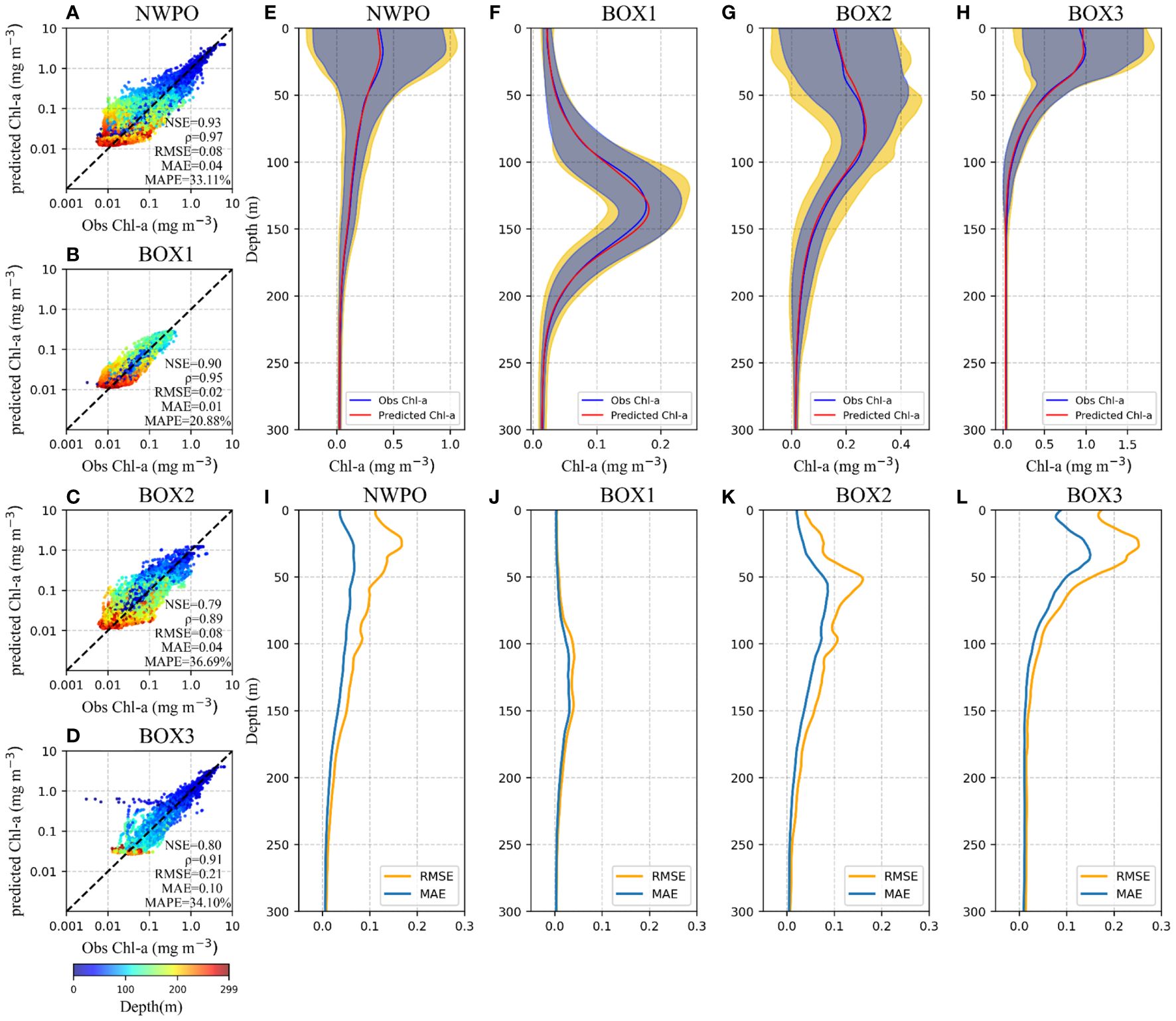
Figure 3 Evaluation of the model’s performance on the test set in the entire NWPO (A, E, I) and three BOXes (B-D, F-H, J-L). (A-D) Scatter plot depicting the observed Chl-a concentration (x-axis) versus the Gaussian-DNN-estimated Chl-a values (y-axis). (E-H) The mean of observed value (blue line) and the mean of DNN predicted values (orange line) in each BOX. The blue and yellow shades are the standard variance of the model results and observations, respectively, which overlap and form the gray shade. (I-L) The RMSE and MAE between observation and model estimates at different depths.

Figure 3 also provides the statistical evaluation of our Gaussian-DNN model. The NWPO and its three sub-regions consistently exhibit high NSE values, ranging from 80% to 90%. This suggests that the input variables, including sea surface Chl-a, depth-resolved water temperature and salinity, can effectively account for the majority of vertical Chl-a variability. The strong correlations (ρ>0.89) coupled with low errors (RMSE<0.21 mg m^-3, MAE<0.10 mg m^-3, and MAPE<37%) indicate that the Gaussian-DNN model accurately captures the vertical structure and magnitudes of Chl-a concentrations in all regions of the NWPO. Additionally, in the three sub-regions, the errors (RMSE, MAE, and MAPE) increase along with latitudes, although MAPE in BOX2 is close to that in BOX3. This trend indicates that the model performs better in low-latitude waters (BOX1) than in higher-latitude waters (BOX2 and BOX3). The observed difference in performance can be attributed, in part, to the varying change rate of Chl-a vertical shape (SCMs characteristics) with latitudes. As illustrated in Figure 4, vertical Chl-a profiles in the tropical region maintain nearly constant SCMs characteristics, while in subtropical and temperate regions, SCMs are more prominent during summer, and surface blooms occur in winter. In summary, this quantitative analysis enhances the credibility of our Gaussian-DNN model outputs in the test set at a daily time scale, demonstrating accuracy and precision.

Figure 4

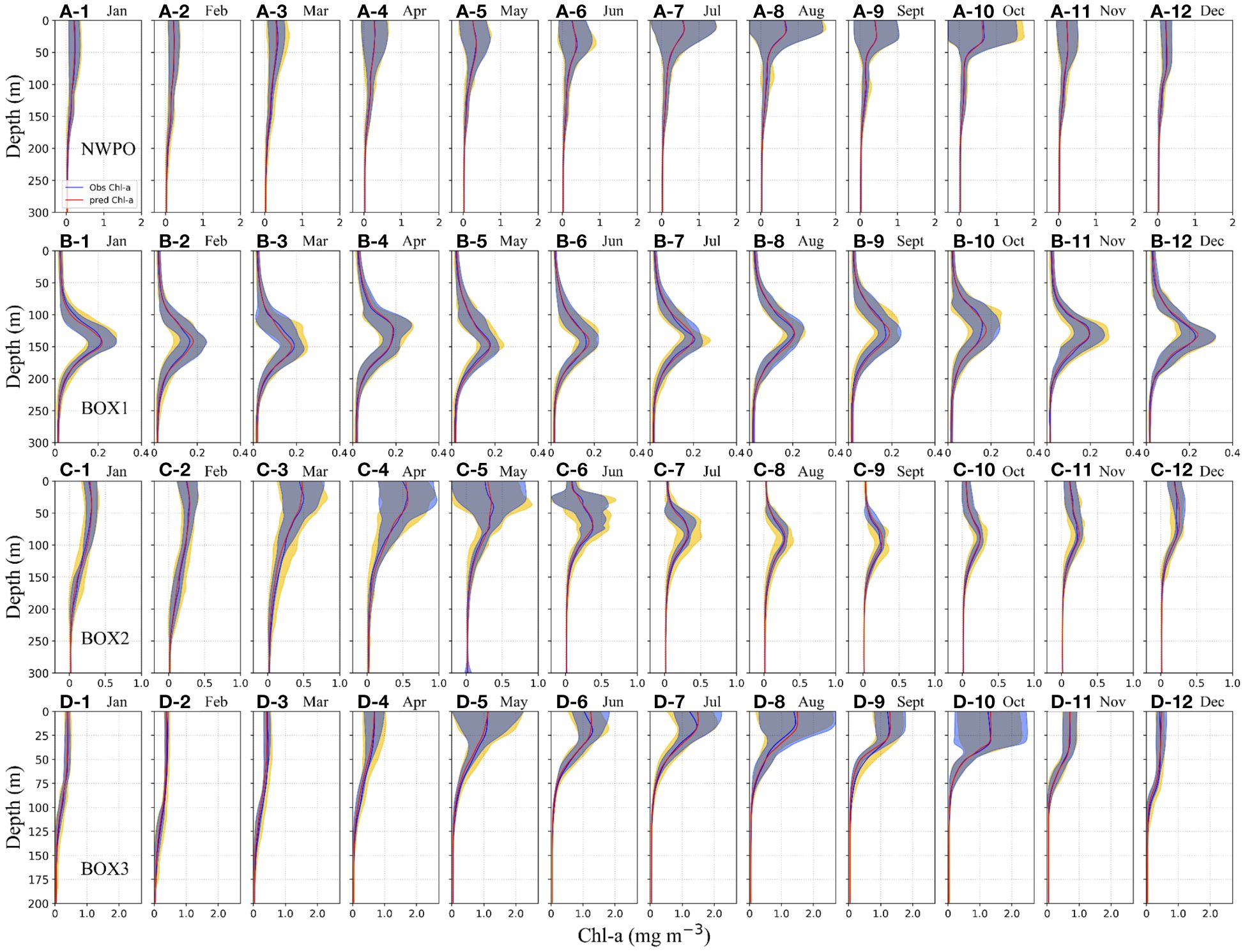
Figure 4 Aggregated Chl-a vertical profiles from the test set in the overall region are in terms of months. The blue and orange solid lines represent the mean of observed value and the mean of Gaussian-DNN predicted Chl-a, respectively. The blue and yellow shades are the standard variance of the model results and observations, respectively, which overlapped and formed the gray shade. (A) Overall area, (B) BOX1 (12–24°N waters), (C) BOX2 (24–38°N waters), and (D) BOX3 (38–54°N waters).

In our modeling results across various water depths, the averaged vertical Chl-a profiles for the NWPO and each sub-region closely mirror their BGC-Argo structures, respectively (Figures 3E-H). More specifically, the Gaussian-DNN results exhibited smaller fluctuations in the surface and SCM layers. The generally low RMSEs (MAEs) within the 0–300 m depth range exhibit maximal values of less than 0.2 mg m^-3 (0.1 mg m^-3) across the entire NWPO (Figure 3I). Within each sub-region, the highest RMSE and MAE are consistently observed within the SCM layers (Figures 3J-L). Additionally, high errors in BOX2 and BOX3 are also observed at the surface layer, with RMSE values close to 0.2 mg m^-3 and MAE up to 0.1 mg m^-3 in BOX3. Such discrepancy may become larger due to higher Chl-a variance within the SCM layer (e.g., the yellow shaded area in Figures 3F-H). Potentially, this will affect network’s prediction accuracy for vertical Chl-a profiles.

Furthermore, we compared monthly averaged Chl-a profiles in the Gaussian-DNN model output with the BGC-Argo (Figure 4). Across the entire NWPO, monthly mean of predicted Chl-a profiles align well with the observed values, especially during the summer and fall seasons (Figures 4A1-12). This suggests that the Gaussian-DNN method effectively captures various types of the vertical Chl-a profiles in the NWPO.

In the tropical sub-region (BOX1), our Gaussian-DNN model effectively reproduced seasonal cycle of the SCM phenomena. Though seasons, SCMs consistently occur near 100–150 m and exhibit an overall low intensity less than 0.3 mg m^-3 (Figures 4B1-12). The predicted mean vertical Chl-a profiles overlapped with observed profiles, along with their corresponding standard variance ranges, demonstrating the effective performance of our model in predicting the SCMs characteristics in the tropical area. In the subtropical sub-region (BOX2), the significant SCMs occur from June to November, with smaller fluctuations in Gaussian-DNN modeling results than observed Chl-a, especially within SCM layers (Figures 4C6-11, green shades). From early winter to late spring, vertical Chl-a profiles in this region exhibit surface blooms, which are well reproduced by the Gaussian-DNN model with smaller shaded areas than observed variance (Figures 4C1-5, C12). Toward higher surface Chl-a concentrations in the temperate gyre (BOX3), the network exhibits a slight overestimation of Chl-a during summer and autumn (Figures 4D6-10), possibly influenced by the high variability of Chl-a values in the upper layer, which poses challenges for accurate predictions, particularly in the upper layers. Overall, the comparison of Gaussian-DNN model outputs with BGC-Argo profiles shows mostly overlapping shaded areas in Figures 4D1-12. This strengthens the ability of the Gaussian-DNN model to integrate, in its response, the variability of the Chl-a field in the NWPO.

Additionally, we conducted a comparative analysis on diverse vertical distributions of Chl-a, involving our Gaussian-DNN alongside MLP and RF methods. In contrast to the Gaussian-DNN model, the MLP model utilizes the Rectified Linear Unit (ReLU) as the activation function and consists of four hidden layers (also named ReLU-DNN). To assess and quantify the enhancement in the performance of Gaussian-DNN model, we employed identical datasets for training and testing across all three models.

Figure 5 presents a radar diagram depicting the relative deviation between MLP, RF, and the Gaussian-DNN model. In comparison with the RF method, MLP exhibits a reduced bias, particularly in mid-to-high latitude regions where relative deviations fall within the range of -13% to 12%. These findings underscore the superior accuracy and performance of the DNN models (Gaussian-DNN, ReLU-DNN) over RF, especially in the high-latitude areas of the NWPO.

Figure 5

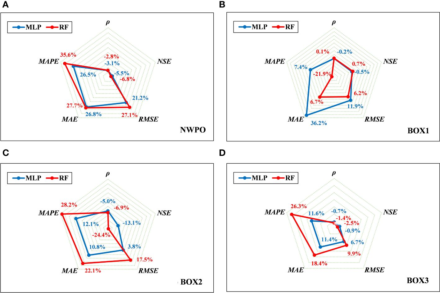
Figure 5 Comparing the MLP, RF and Gaussian-DNN performance in the test set by the Radar diagram of relative deviations in the NWPO (A) and three sub-regions (B-D).

When contrasting the results of our Gaussian-DNN model with that of MLP in the NWPO (Figure 5A), we observed a slight decrease (less than 5.5%) in the values of NSE and ρ. Meanwhile, RMSE, MAE, and MAPE displayed a more significant increase, reaching up to 26.8%. Specifically, in tropical waters the disparities in outcomes among these three models are negligible, except for the MAE derived from the MLP model (Figure 5B). This variation is attributed to the small MAE values observed in the tropical gyre, approximately (~0.01 mg m^-3). However, as we move to higher latitudes (Figures 5B, C), particularly in subtropical waters, the disparities in outcomes among these three models become more pronounced (from -24.4% to 28.2%). These findings suggest that the utilization of the Gaussian activation function has a positive impact on the accuracy of Chl-a estimation than that of ReLU. It is noteworthy that the improvement aligns with the results obtained by Chen et al. (2022a), who reported similar enhancements when comparing the Gaussian function with the Sigmoid activation. This consistency across studies underscores the effectiveness of the Gaussian activation function in refining the accuracy of Chl-a estimation.

3.2 Robustness validation of Gaussian-DNN on independent data sets

To evaluate the generalization and robustness of our trained Gaussian-DNN model, we applied it to estimate Chl-a concentrations using ship measurements from JMA. The JMA data, including Chl-a, temperature, salinity, were input into the trained Gaussian-DNN model using JMA data, while maintaining the same training and test sets initially utilized with the BGC-Argo data. The identical statistical parameters utilized to evaluate the model’s performance with the BGC-Argo data were also applied to assess its performance with the JMA dataset. The statistical indicators in Table 2 are comparable to those obtained by the trained Gaussian-DNN for the entire NWPO (refer to Figure 3A), indicating that our Gaussian-DNN model maintains robust performance across different datasets. The slight discrepancy may be attributed to the ship survey data having fewer profile sample points and a potential limitation in capturing deep Chl-a profile features.

Table 2

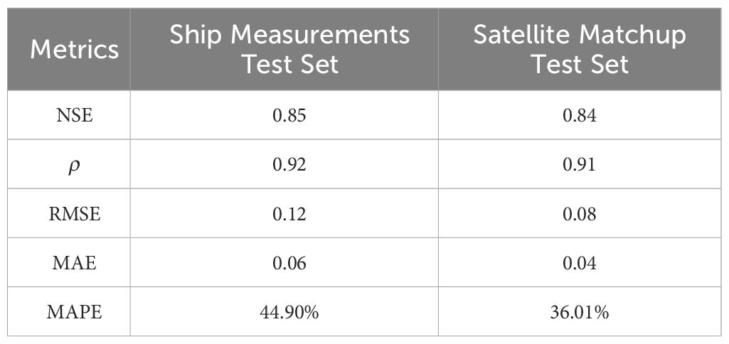
Table 2 The statistical results obtained from the validation model using JMA hydrological data.

Furthermore, two transects were selected to demonstrate the model effectiveness, as indicated in Figure 1B by the two red vertical dashed lines representing the 137°E and 165°E transects. When compared to ship measurements, the Gaussian-DNN model successfully reproduced the vertical distribution of Chl-a along the 137°E section, with most differences falling within the range of -0.1 to 0.1 mg m^-3 (Figures 6A-C). The predicted values for the 165°E section correspond well to the observed values (Figures 6D-F). However, relatively large deviations (0.2 to 0.3 mg m^-3) are mainly observed at high latitudes above 40°N, such as 40°N, 44°N, and 48°N. These discrepancies could stem from variations in the input data sourced from JMA and BGC-Argo (Supplementary Figure 4). For example, water temperatures between 2–5°C recorded by JMA appear lower compared to those derived from BGC-Argo floats, particularly evident in areas above 40°N along 165°E (Supplementary Figure 5). Additionally, there are similar observations regarding salinity levels, where values between 32–36 from JMA are notably lower than those recorded by BGC-Argo floats, especially in regions above 40°N along 165°E (Supplementary Figure 5). Overall, the performance of the trained Gaussian-DNN model is satisfactory when tested with ship measurement data.

Figure 6

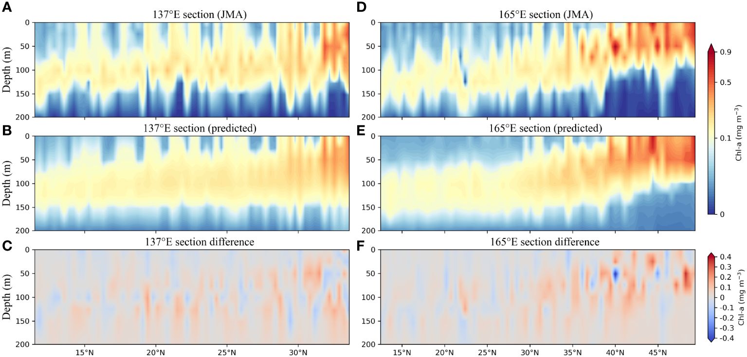
Figure 6 Vertical distribution of Chl-a concentrations along the 137°E section derived from (A) observation data and (B) the model estimates. (C) The difference between (A, B). (D-F) Same as (A-C) but along the 165°E section.

3.3 Reconstruction of long-term 3-D Chl-a structure

To project the long-term 3-D Chl-a structure in the NWPO, the MODIS Chl-a and BOA-Argo global gridded thermohaline data were merged as the input dataset in the deployment phase of the trained Gaussian-DNN model. The reconstructed monthly 3-D structure of Chl-a in the NWPO has a spatial resolution of 1°×1° with fully depth-resolved vertical profiles in 0–300 m layer, covering the period from January 2004 to June 2022.

We conducted a comparative analysis to evaluate the performance of Gaussian-DNN on 3-D structures and backward time-series prediction. Figure 7A showed the DNN-estimated surface Chl-a values against MODIS observed ones. A high density of data points is concentrated around the bisector, especially in the range from 0.01 to 0.1 mg m^-3. On contrary, the scatter increases in the higher domain of Chl-a concentrations, in which the data density is reduced (Figure 7A), revealing an underestimation of the Gaussian-DNN predicted values in BOX3 (see Figures 7H-J). The main factor contributing to this discrepancy is likely the potential uncertainties in gap filling for missing MODIS Chl-a data, particularly influenced by the high solar zenith angle, which tends to affect prediction accuracy in high-latitude waters (Supplementary Figure 6). In depicting the time-series patterns of surface Chl-a spanning the entire decade from 2004 to 2022, our Gaussian-DNN models effectively capture the observed seasonal and interannual variations from MODIS, despite an overall slight overestimation of 0.1 mg m^-3 (Figure 7K). It is noteworthy that we trained the Gaussian-DNN models using data from the period of 2017–2022, extending backward to 2004 during the deployment phase. This outcome underscores the impressive generalization ability of our Gaussian-DNN model.

Figure 7

Figure 7 (A) Density plot of DNN-reconstructed surface Chl-a values against MODIS values. Monthly vertical Chl-a from 2004 to 2022 in (B–D) BOX1, (E–G) BOX2, and (H–J) BOX3 from BGC-Argo (top panel), Gaussian-DNN model (middle panel), and the differences between them (Gaussian-DNN model outputs minus BGC-Argo, bottom pane), respectively. (K) Comparison of Gaussian-DNN reconstruction results with time-series patterns of sea surface Chl-a from MODIS and BGC-Argo observations for the period 2004–2022.

The vertical patterns of reconstructed Chl-a by the Gaussian-DNN model align closely with those observed by the BGC-Argo floats within the 0–300 m layer (Figures 7B-J). In the tropical region (BOX1), the predicted Chl-a values with a prominent SCM in all seasons closely match the measurements obtained from BGC-Argo float data (Figures 7B-D). Within the subtropical gyre of the NWPO (BOX2), a dynamic interplay between surface blooms and the SCMs characterizes the seasonal cycle. Our Gaussian-DNN model has demonstrated its capability to accurately reproduce both blooms in the surface and subsurface layer (Figures 7E-G). In the temperate region (BOX3), our Gaussian-DNN model demonstrates a high level of accuracy in capturing Chl-a patterns as observed in BGC-Argo data. However, it consistently tends to slightly underestimate the Chl-a values in the 0–50 meter depth range, particularly during the months of July to September (Figures 7H-J). This deviation is likely attributed to disparities in input data sources used for reconstruction (MODIS) and training (BGC-Argo) (see Figure 7K; Supplementary Figure 1).

Furthermore, the same statistical indicators that was used for the overall evaluation of the Gaussian-DNN performance were considered (see satellite matchup set in Table 2). The NSE (0.85) was close to those obtained on BGC-Argo (0.93) and ship measurements (0.84), indicating the effectiveness of input variables on predicting Chl-a. The others statistical parameters, ρ=0.91, RMSE = 0.08 mg m^-3 and MAE = 0.04 mg m^-3, were of the same order of magnitude of those obtained on test sets of BGC-Argo and ship measurements (Figures 3A–D; Table 2). Analogous results were obtained in previous and similar works as, e.g., that of Hu et al. (2023), in which the vertical profile of Chl-a in the Northern India Ocean is inferred by the combined use of 18 input variables from BGC-Argo and satellite data in the RF model, obtaining an NSE and RMSE of 0.96 and 0.01 mg m^-3, respectively. The comparison of our statistical results with those of Hu et al. (2023) highlighted that, even with some uncertainties and some limits, our network, applied on 7 out of 18 input variables shows a prediction accuracy very close to other models. Overall, the validation confirms that the Gaussian-DNN model serves as an effective tool for generating long-term, 3-D Chl-a data by merging satellite Chl-a information and temperature-salinity float profiles.

3.4 Spatio-temporal patterns of SCMs characteristics

Using the reconstructed long-term 3-D Chl-a profiles in the NWPO, we calculated the depth of the Chl-a maximum in each individual profile which has the 1 m vertical resolution. Here, we designated the peak Chl-a value in each individual profile as SCMs intensity and identified its location as SCMs depth, taking advantage of the notably high vertical resolution. Subsequently, we assessed the spatio-temporal variability of SCMs characteristics (depth and intensity).

Spatially, the intensity of SCMs exhibits a distinct upward trend across latitude zones (Figure 8A), ranging from 0.21±0.03 mg m^-3 in the tropical gyre to 0.36±0.16 mg m^-3 in subtropical waters, and peaking at 0.79±0.50 mg m^-3 in the temperate area. Concurrently, the SCMs depth decreases with higher latitude zones, measuring 121 ± 17 m, 54 ± 31 m, and 13 ± 14 m, respectively. A distinct transition band was evident between the high intensity of SCMs temperate waters and the low-intensity subtropical waters (Figures 8A, B). The geographical location of subsurface Chl-a transition bands near the Kuroshio–Oyashio convergence region exhibited seasonal migration dynamics, extending equatorward in spring and summer and shifting poleward in fall and winter. In parallel, the majority of oligotrophic subtropical and tropical waters began expanding in the late summer, reached their spatial maximum in the autumn, and then contracted in the winter and spring.

Figure 8

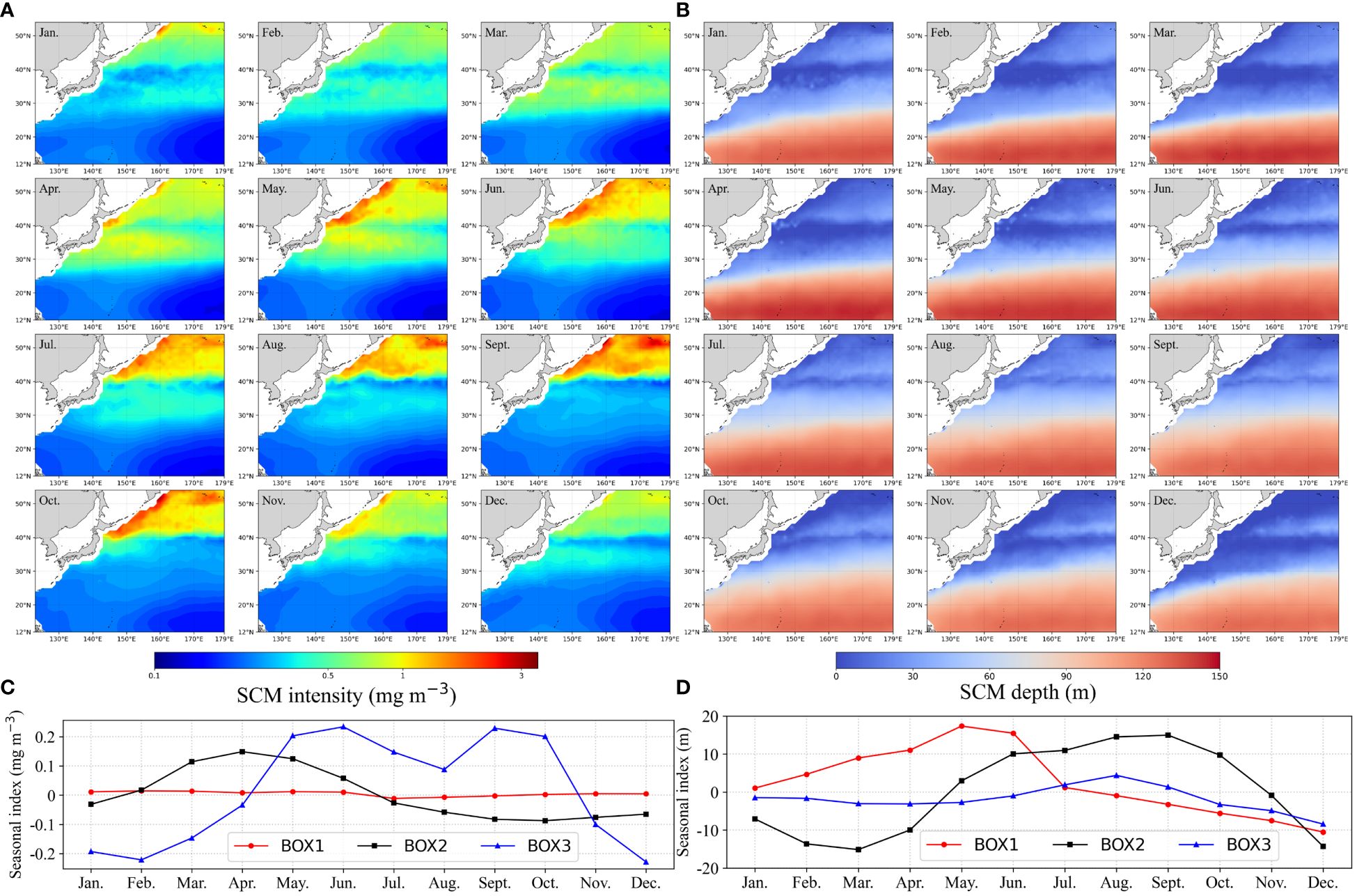
Figure 8 Climatological monthly SCMs intensity (A) and SCMs depth (B) in the NWPO and the corresponding seasonal indices of SCMs intensity (C) and SCMs depth (D).

The seasonal indices were calculated using an additive decomposition model (Hyndman and Athanasopoulos, 2021), with the calculation formula represented by (Supplementary Equation S2). SCMs exhibit distinct patterns in both intensity and depth (Figures 8C, D), showcasing intriguing seasonal variations across different regions. Within temperate waters, SCMs intensity displays bi-modal peaks from late spring through early fall, featuring a shallow SCM during summer (Figures 8C, D). Conversely, subtropical waters experience a singular peak in SCMs intensity during spring, with the deepest SCM recorded in the fall (Figures 8C, D). In tropical oligotrophic waters, while the SCMs intensity remains stable, there are noticeable seasonal variations in SCMs depth, with the shallowest SCMs occurring in May and the deepest in December (Figure 8D).

3.5 Long-term trend of total Chl-a during 2004–2022

To broaden insights beyond surface-level observations, we conducted an assessment of the long-term trends in total Chl-a within the water column. This involved computing the monthly mean of depth-integrated Chl-a within the 0–300 m depth range, utilizing the reconstructed monthly 3-D Chl-a data in the NWPO from 2004 to 2022. Subsequently, we evaluated the trends of total Chl-a using a Locally Weighted Scatterplot Smoothing (LOWSS) method (Cleveland et al., 1990). The LOWSS smoother operates by fitting a weighted polynomial regression for a given time of observation, with weights decreasing as the distance from the nearest neighbor increases (Dagum and Luati, 2003). This approach enables us to separate the seasonal component from the trend component, providing a deseasonalized trend component (Supplementary Figure 7).

The average depth-integrated Chl-a in the NWPO for the period 2004–2022 stood at 35 ± 19 mg m^-2, exhibiting noteworthy spatial distinctions across the tropical (20 ± 4 mg m^-2), subtropical (36 ± 13 mg m^-2), and temperate (55 ± 20 mg m^-2) gyres. For the long-term time series analysis, the depth-integrated Chl-a exhibits significant interannual variability in the NWPO during the period of 2004–2022, with notable linear trends observed in tropical and subtropical gyres (Figure 9). For instance, the depth-integrated Chl-a in the tropical gyre shows a minimum in 2007 and a peak value in 2009. On average, the depth-integrated Chl-a in the tropical region exhibits an increasing trend of 0.0016 mg m^-2 yr^-1 (p=0.05). In the subtropical region, a more pronounced decreasing trend of 0.0033 mg m^-2 yr^-1 is observed (p<0.01). However, no significant linear trend is found in the temperate area (p=0.12). To provide a detailed depiction of the spatial distribution of long-term variations in the NWPO, we calculated the linear trend for each pixel (Figure 9G). Noted that all trends mentioned in the following sections are statistically significant at a significance level of p< 0.05.

Figure 9

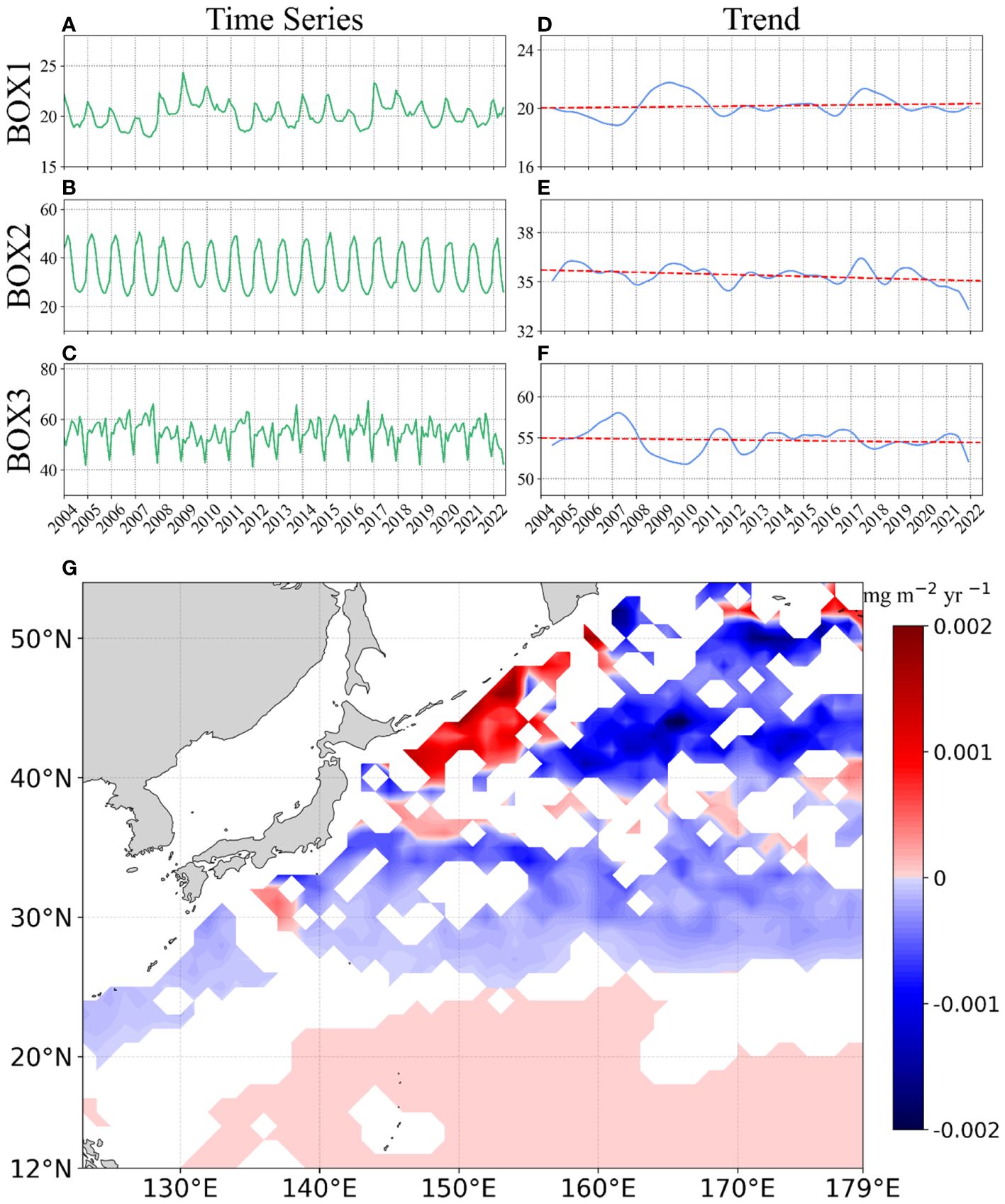
Figure 9 (A-C) Time series of depth-integrated Chl-a in three BOXes of the northwest Pacific Ocean during the period of 2004–2022. (D-F) Interannual variation of depth-integrated Chl-a in three BOXes. (G) Spatial pattern of trends (unit: mg m^-2 yr^-1) of depth-integrated Chl-a. Warm colors indicate positive trends, cold colors represent negative trends, and white signifies no detected trends. Note that only data that passed the confidence tests (p< 0.05) were displayed.

The locations with significant increasing (decreasing) patterns in depth-integrated Chl-a exhibit a patchy distribution (Figure 9G). Predominantly, increasing trends were observed in the tropical gyre, while negative trends were notable in the subtropical section. In the temperate gyre, originating from the marginal seas, continuous patches with increasing depth-integrated Chl-a extended toward the northeast in the NWPO, forming a nearly contiguous belt with positive interannual trends. Off the Sea of Okhotsk, patches with positive depth-integrated Chl-a trends were consistently distributed along the chain of islands, exhibiting an annual increasing rate of ~0.002 mg m⁻² yr⁻¹. Further northeast, similar patches with increasing depth-integrated Chl-a were observed off the southern region of the Bering Sea. However, in the remaining part of the temperate gyre, the depth-integrated Chl-a exhibited a decreasing trend at a rate of ~-0.002 mg m⁻² yr⁻¹. Overall, the linear trend across the entire temperate area was not found to be statistically significant.

4 Discussion

4.1 Sensitivity of input variables

As a data-driven model, the effectiveness of a DNN is notably influenced by the selection of input variables (Reichstein et al., 2019). We conducted a series of sensitivity experiments for three watersheds to examine how sea surface Chl-a and vertical physical properties (water temperature and salinity) influence the accuracy of our estimations. In each experiment, only one input variable was removed, keeping the other input variables unchanged.

As depicted in Table 3, in Exp-without T, where we removed the temperature variable, a notable reduction in model performance is observed, particularly in low-latitude seas, with the RMSE decreasing by 17.62% and the MAE decreasing by 13.71%. In mid- and high-latitude waters (BOX2 and BOX3), the influence of water temperature on the estimated Chl-a profiles appears to be less significant. In Exp-without S, the reduction in model performance after removing salinity was not as substantial as when temperature was removed. The influence of salinity was only observed to some extent in mid- and high-latitude waters (less than 5%). Nonetheless, the significance of salinity’s contribution to the model’s effectiveness should not be overlooked.

Table 3

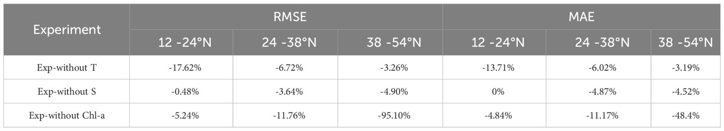
Table 3 Relative deviation of sensitivity experiments from the trained Gaussian-DNN models with Root Mean Square Error (RMSE) and Mean Absolute Error (MAE).

When sea surface Chl-a was removed in Exp-without Chl-a, the model performance in the three sub-regions was diminished, particularly in the high-latitude gyre. The RMSE decreased by 5.24%, 11.76%, and 95.10%, respectively, and the MAE also exhibited varying degrees of reduction from 4.84% to 48.4% along latitude increasing (Table 3). This underscores the substantial contribution of sea surface Chl-a as an input variable to the Gaussian-DNN model, especially in the temperate waters with high Chl-a concentrations.

Generally, vertical distribution of water temperature plays a more important role in estimation of Chl-a in comparison with salinity in tropical and subtropical gyres of the NWPO; for the temperate areas, the latter is more essential than the former. This is consistent with the understanding from the in situ observations. For example, in the tropical area of NWPO the everlasting SCMs were found in the vicinity of the thermocline, consisting with the nitracline, hence being of an essential feature of the typical tropical structure (Herbland and Voituriez, 1979; Cullen, 1982; Radenac and Rodier, 1996; Cullen, 2015). While in the high- latitude waters, observations revealed that the vertical distribution of Chl-a that was closely related to the seasonal evolution of halocline and pycnocline (Anderson, 1969; Ishida et al., 2009).

In addition, the sensitivity results illustrate that the vertical physical properties should be deliberated in reconstructing the vertical Chl-a profiles. Analogous results have been found in northern India Ocean (Hu et al., 2023). Compared with previous studies applied on surface measurements only (SST and surface Chl-a), adding vertical physics properties (water temperature and salinity) as input variables leads the NSE increasing from ~70% to ~90% (Sammartino et al., 2018; Chen et al., 2022a; Wang et al., 2023a). Here, we emphasize that in the tropical area of the NWPO, surface Chl-a and vertical temperature profiles are two effective input variables in accurately estimating vertical Chl-a profiles. For the high-latitude waters, both vertical profiles of temperature and salinity together with surface Chl-a are non-negligible.

4.2 Variability discrepancy between subsurface Chl-a and surface Chl-a

It is well-established that the satellite record effectively captures global phytoplankton responses but is confined to present changes in the surface ocean environment. However, the presence of SCMs necessitates caution when extrapolating conclusions from the surface to water-column-integrated production or when predicting potential impacts of future ocean warming (Behrenfeld et al., 2016).

The characteristics of SCMs in the NWPO demonstrate significant spatial variability along with seasonal fluctuations during 2004–2022 (Figure 8). This spatial variability of SCMs characteristics closely resembles the observed patterns in surface Chl-a levels based on ocean color data in the NWPO (Hou et al., 2016; Chen et al., 2022b). As latitudes increase, SCMs intensity (its depth) also tends to increase (decrease), leading to the formation of a distinct transition band between the high intensity of SCMs in temperate waters and the low-intensity subtropical waters (Figures 8A, B). This transition band has also been noted in the spatial patterns of surface Chl-a (Chen et al., 2022b). During cold seasons (winter and spring), the transition band of subsurface Chl-a extends equatorward, while during warm seasons (summer and fall), it shifts poleward. This seasonal migration correlates with variations in the strength of the Kuroshio Extension surface transport and its associated southern recirculation (Qiu et al., 2014; Yang and Liang, 2018). Notably, the seasonal migration pattern of the transition band of subsurface Chl-a differs from that of surface Chl-a, with the surface transition band moving equatorward in fall and winter, and poleward in spring and summer (Chen et al., 2022b). Further exploration is needed to understand the reasons for this discrepancy in seasonal cycles between subsurface and surface Chl-a transition bands.

For the seasonality, the dual peaks of SCM intensity in the temperate waters during spring and autumn (Figure 8C) are mainly triggered by reduced vertical stability (Bailey and Werdell, 2006). Due to intensified vertical mixing in early winter, phytoplankton in the SCM layer is entrained upward to the surface mixed layer, leading to enhanced surface Chl-a during this period (Behrenfeld and Boss, 2014; Lacour et al., 2019; Xing et al., 2020). For the subtropical gyre, the initiation of high values in SCMs intensity during spring resembled that observed in temperature oceans (Figure 8C). This occurrence can be attributed to sufficient nutrients brought to the ocean upper layer by previous wintertime mixing, higher temperature, light and vertical stability conditions (Sverdrup, 1953; Siegel, 2002). During summertime, the mixed layer depths were notably shallow, and robust stratification confined nutrient supplementation within the subsurface layer, resulting in evaluations of ecological significance of SCMs (Furuya, 1990; Venrick, 1993). In the tropical NWPO, the existence of a permanent halocline and pycnocline, hinders the vertical transport of nutrient-rich deep water to the nutrient-exhausted surface mixed layer, giving rise to a persistent SCM throughout the year (Anderson, 1969; Cullen, 2015). Consequently, the SCMs intensity shows minimal seasonal variations in the tropical gyre of the NWPO.

In general, the seasonal dynamics of subsurface Chl-a resembled those observed in surface Chl-a based on ocean color data in the NWPO (Hou et al., 2016; Chen et al., 2022b). However, there is a temporal disparity in the onset of seasonal peaks between the surface layer and subsurface layer. As shown in Figures 8C, D, there is a two-month delay in the intensity of SCMs as latitude increases. In contrast, the surface bloom exhibits a one-month delay (Chen et al., 2022b). For instance, in the subtropical gyre, the maximal SCMs intensity is reached in March, extending into May in temperate waters. In comparison, the surface bloom extends from March in subtropical waters to April in the temperate gyre (Chen et al., 2022b). This temporal discrepancy is likely attributed to the response of phytoplankton to factors such as light availability and water stratification. The observed patterns underscore the intricate interplay between environmental factors and phytoplankton dynamics in shaping the seasonal variability of Chl-a in both surface and subsurface layers of the NWPO.

Furthermore, we conducted a comparative analysis of the long-term trends of Chl-a in the surface layer and depth-integrated Chl-a within the water column of the NWPO. Notably, distinct trends between depth-integrated Chl-a and surface Chl-a were observed across the NWPO. For instance, during the period from 2004 to 2022, the estimated depth-integrated Chl-a exhibited opposite trends in the tropical and subtropical regions, with a more significant decreasing tendency observed in the latter region (Figure 9). Conversely, no significant trend in surface Chl-a was observed in the subtropical water during 1997–2020 (Chen et al., 2022b), while a clear positive trend was evident in the tropical water (Chen et al., 2022b; Yu et al., 2023). Moving toward higher latitude waters (BOX3, Figure 9G), our analysis revealed increasing interannual trends for depth-integrated Chl-a in parts of the temperate section, which aligned with trends noted in remote-sensing Chl-a (Chen et al., 2022b). This disparity between the trends of depth-integrated Chl-a and surface Chl-a can be attributed to the presence of SCMs in the tropical and subtropical gyres, which contrasts with the near-surface blooms observed in the temperate gyre of the NWPO.

4.3 Uncertainties and implication in 3-D Chl-a reconstruction

In this study, vertical physical properties such as water temperature and salinity within the 0–300 m water depth were utilized as crucial predictors. These properties are essential for accurately predicting vertical Chl-a profiles in the NWPO (Table 3) as they govern the availability of nutrients for phytoplankton across different layers of the water column. The fluctuations in thermohaline observations directly influence the prediction of Chl-a concentrations. For example, significant variations were observed in the vertical distributions of temperature and salinity in three profiles from Float 2903354 in BOX3 compared to other locations (Supplementary Figure 8). This discrepancy resulted in predicted Chl-a values within the upper 100 m depth that were notably higher than the observed values, leading to several scattered points between 0.1 and 1 mg m^-3 on the y-axis exhibiting considerable deviation from the 1:1 line, indicative of a nearly horizontal distribution (Figure 3D). In addition, the uncertainties associated with thermohaline profiles from BGC-Argo and BOA-Argo floats significantly influence the accuracy of our developed Gaussian-DNN model, particularly noticeable in the temperate gyre of the NWPO. For instance, in the tropical gyre, there is an evident upwelling in April presented by BGC-Argo (Supplementary Figure 9), resulting in a shoaling SCM (Figure 7), while a constantly reconstructed SCM based on stable stratification is presented by BOA-Argo (Supplementary Figure 9). In the temperate waters, salinities from BOA-Argo are higher than those from BGC-Argo in the 0–50 m depth, especially during summer and autumn seasons (Supplementary Figure 9), leading to an overestimation of Chl-a in the upper layer (Figure 7J).

To further assess the model’s sensitivity to the uncertainty of input physical variables, we conducted eight experiments in each BOX region. Specifically, we introduced temperature uncertainties of ±0.2°C within both the surface 20 meters and the depth range of 0–300 meters. For salinity, uncertainty was assumed to be ±1% of the average surface values in each BOX region, resulting in values of ±0.349, ± 0.345, and ±0.328, respectively. The results, depicted in Supplementary Figure 10, reveal that slight variations in temperature or salinity have a negligible effect on the model’s performance compared to its original state in BOX1. However, In BOX2 and BOX3, we observed a notable increase in RMSEs above a depth of 150 meters. This suggests that even minor variations in water temperature and salinity occurring within the surface layer, can have a significant impact on the performance of our DNN model in these regions. This finding underscores the significance of water temperature and salinity as critical predictors for vertical Chl-a profiles, particularly in mid- and high-latitude waters.

Furthermore, the accuracy of surface Chl-a is a crucial input variable that significantly impacts the reconstruction outcomes, particularly in temperate waters (Table 3). Two main uncertainties are associated with surface Chl-a. One arises during the preprocessing of surface Chl-a derived from different datasets (BGC-Argo and MODIS data). To address this, we conducted a retraining of the Gaussian-DNN model. This involved incorporating half of the Chl-a values from BGC-Argo in BOX3 while leaving the rest of the training data unchanged. The results showed a significant reduction in disparities between our Gaussian-DNN model and the MODIS (refer to Supplementary Figure 11), which also helps clarify the overestimation illustrated in Figure 7K.

The other significant source of uncertainty arises from the gap filling process of MODIS data, particularly pronounced in high-latitude waters where the missing rate of MODIS Chl-a data tends to be higher (refer to Supplementary Figure 2). The accuracy of this filling process may be compromised by the elevated solar zenith angle prevalent in these regions, thereby influencing prediction accuracy. To address this, we conducted a re-run of the Gaussian-DNN model by masking the missing MODIS data. The resulting density scatter plot revealed the disappearance of the severe underestimation for high Chl-a concentration in Figure 6A (see Supplementary Figure 6), highlighting the influence of interpolation uncertainty on the accuracy of Chl-a reconstruction. Therefore, integrating a diverse range of Chl-a data sources, such as individual satellites like MODIS, SeaWiFS, MERIS, and VIIRS, as well as composite satellite products like OC-CCI, and enhancing the accuracy of gap filling techniques, can help to improve the performance of our Gaussian-DNN model in reconstructing long-term 3-D Chl-a structures.

With the continuous and anticipated future availability of spatio-temporal depth-resolved physics datasets, the prospect of developing long-term 3-D global Chl-a datasets is becoming feasible. This product is positioned to comprehensively capture the multifaceted changes expected with upcoming climate change, offering a holistic understanding of phytoplankton dynamics across different dimensions of the water column.

5 Conclusion

In this study, we developed a Gaussian-DNN model to construct long-term 3-D Chl-a structures by inputting satellite Chl-a with BOA-Argo thermohaline profiles, featuring a spatial resolution of 1°×1° and a vertical resolution of 1 m within the 0–300 m water depth from 2004 to 2022 in the NWPO. The trained Gaussian-DNN model using BGC-Argo float data was successfully applied to JMA ship measurements, demonstrating its robust generalization ability. The experiments for input sensitivity demonstrated a crucial role of ocean water temperatures in estimating Chl-a in the subtropical gyre, while a switch to salinity in the temperate gyre. The estimated SCMs in the NWPO exhibited spatial divergence of significant seasonality. Opposing trends of total Chl-a in water columns were observed in the tropical and subtropical gyres during 2004–2022, insignificant trend was characterized in the temperate area, mostly attributed to spatial discrepancies in tendencies. Overall, the developed Gaussian-DNN model, alongside the growing availability of thermohaline datasets, holds significant promise for constructing long-term 3-D Chl-a in the NWPO, offering comprehensive insights into the multifaceted changes expected in future climate change scenarios.

Data availability statement

The raw data supporting the conclusions of this article will be made available by the authors, without undue reservation.

Author contributions

XZ: Data curation, Formal analysis, Investigation, Methodology, Software, Validation, Visualization, Writing – original draft. XiaG: Conceptualization, Formal analysis, Funding acquisition, Investigation, Methodology, Project administration, Resources, Validation, Writing – review & editing. XunG: Formal analysis, Funding acquisition, Writing – review & editing. JL: Data curation, Formal analysis, Methodology, Writing – review & editing. GW: Data curation, Formal analysis, Methodology, Writing – review & editing. LW: Data curation, Formal analysis, Methodology, Writing – review & editing. XinG: Data curation, Formal analysis, Writing – review & editing. HG: Formal analysis, Funding acquisition, Supervision, Writing – review & editing.

Funding

The author(s) declare financial support was received for the research, authorship, and/or publication of this article. This work was supported by the Ministry of Science and Technology of the People’s Republic of China (2019YFE0125000), National Nature Science Foundation of China-Shandong Joint Fund (U1906215), and the National Natural Science Foundation of China (41406010). This work was also supported by the Key Laboratory of Coastal Environmental Processes and Ecological Remediation, Chinese Academy of Sciences Opening Fund (2020KFJJ04).

Acknowledgments

The authors would like to thank the International Argo Program and the China Argo Real-Time Data Center that contribute to the BGC-Argo data and BOA-Argo, which were collected and made freely available. The Argo Program is part of the Global Ocean Observing System. The authors are very grateful to Jianqiang Chen for his helpful advices.

Conflict of interest

The authors declare that the research was conducted in the absence of any commercial or financial relationships that could be construed as a potential conflict of interest.

Publisher’s note

All claims expressed in this article are solely those of the authors and do not necessarily represent those of their affiliated organizations, or those of the publisher, the editors and the reviewers. Any product that may be evaluated in this article, or claim that may be made by its manufacturer, is not guaranteed or endorsed by the publisher.

Supplementary material

The Supplementary Material for this article can be found online at: https://www.frontiersin.org/articles/10.3389/fmars.2024.1378488/full#supplementary-material

References

Alvera-Azcárate A., Barth A., Rixen M., Beckers J. M. (2005). Reconstruction of incomplete oceanographic data sets using empirical orthogonal functions: application to the Adriatic Sea surface temperature. Ocean Model. 9, 325–346. doi: 10.1016/j.ocemod.2004.08.001

CrossRef Full Text | Google Scholar

Anderson G. C. (1969). Subsurface chlorophyll maximum in the northeast Pacific Ocean. Limnol. Oceanogr. 14, 386–391. doi: 10.4319/lo.1969.14.3.0386

CrossRef Full Text | Google Scholar

Anderson S. I., Barton A. D., Clayton S., Dutkiewicz S., Rynearson T. A. (2021). Marine phytoplankton functional types exhibit diverse responses to thermal change. Nat. Commun. 12, 1–9. doi: 10.1038/s41467-021-26651-8

PubMed Abstract | CrossRef Full Text | Google Scholar

Bailey S. W., Werdell P. J. (2006). A multi-sensor approach for the on-orbit validation of ocean color satellite data products. Remote Sens. Environ. 102, 12–23. doi: 10.1016/j.rse.2006.01.015

CrossRef Full Text | Google Scholar

Beckers J. M., Rixen M. (2003). EOF calculations and data filling from incomplete oceanographic datasets. J. Atmos. Ocean. Technol. 20, 1839–1856. doi: 10.1175/1520-0426(2003)020<1839:ECADFF>2.0.CO;2

CrossRef Full Text | Google Scholar

Beckmann A., Hense I. (2007). Beneath the surface: Characteristics of oceanic ecosystems under weak mixing conditions—a theoretical investigation. Prog. Oceanogr. 75, 771–796. doi: 10.1016/j.pocean.2007.09.002

CrossRef Full Text | Google Scholar

Behrenfeld M. J. (2001). Biospheric primary production during an ENSO transition. Science 291, 2594–2597. doi: 10.1126/science.1055071

PubMed Abstract | CrossRef Full Text | Google Scholar

Behrenfeld M. J., Boss E. S. (2014). Resurrecting the ecological underpinnings of ocean plankton blooms. Annu. Rev. Mar. Sci. 6, 167–194. doi: 10.1146/annurev-marine-052913-021325

CrossRef Full Text | Google Scholar

Behrenfeld M. J., O’Malley R. T., Boss E. S., Westberry T. K., Graff J. R., Halsey K. H., et al. (2016). Revaluating ocean warming impacts on global phytoplankton. Nat. Climate Change 6, 323–330. doi: 10.1038/nclimate2838

CrossRef Full Text | Google Scholar

Bittig H. C., Maurer T. L., Plant J. N., Schmechtig C., Wong A. P. S., Claustre H., et al. (2019). A BGC-argo guide: planning, deployment, data handling and usage. Front. Mar. Sci. 6. doi: 10.3389/fmars.2019.00502

CrossRef Full Text | Google Scholar

Bouman H. A., Jackson T., Sathyendranath S., Platt T. (2020). Vertical structure in chlorophyll profiles: influence on primary production in the Arctic Ocean. Phil. Trans. R. Soc. A. 378, 20190351. doi: 10.1098/rsta.2019.0351

CrossRef Full Text | Google Scholar

Chen J., Gong X., Guo X., Xing X., Lu K., Gao H., et al. (2022a). Improved perceptron of subsurface chlorophyll maxima by a deep neural network: A case study with BGC-argo float data in the Northwestern Pacific ocean. Remote Sens. 14, 632–632. doi: 10.3390/rs14030632

CrossRef Full Text | Google Scholar

Chen S., Meng Y., Lin S., Xi J. (2022b). Remote sensing of the seasonal and interannual variability of surface chlorophyll-a concentration in the Northwest Pacific over the past 23 years, (1997–2020). Remote Sens. 14, 5611–5611. doi: 10.3390/rs14215611

CrossRef Full Text | Google Scholar

Chikuni S. (1986). The fish resources of the northwest Pacific. Internation. Rev. der gesamten Hydrobiol. und Hydrogr. 71, 840–840. doi: 10.1002/iroh.19860710611

CrossRef Full Text | Google Scholar

Cleveland R. B., Cleveland W. S., McRae J. E., Terpenning I. (1990). STL: A seasonal-trend decomposition procedure based on Loess. J. Off. Stat. 6, 3–73.

Google Scholar

Colella S., Falcini F., Rinaldi E., Sammartino M., Santoleri R. (2016). Mediterranean ocean colour chlorophyll trends. PloS One 11, e0155756. doi: 10.1371/journal.pone.0155756

PubMed Abstract | CrossRef Full Text | Google Scholar

Cornec M., Claustre H., Mignot A., Guidi L., Lacour L., Poteau A., et al. (2021). Deep chlorophyll maxima in the global ocean: occurrences, drivers and characteristics. Global Biogeochem. Cycles 35, 1–30. doi: 10.1029/2020GB006759

CrossRef Full Text | Google Scholar

Cullen J. J. (1982). The deep chlorophyll maximum: comparing vertical profiles of chlorophyll a. Can. J. Fish. Aquat. Sci. 39, 791–803. doi: 10.1139/f82-108

CrossRef Full Text | Google Scholar

Cullen J. J. (2015). Subsurface chlorophyll maximum layers: enduring enigma or mystery solved? Annu. Rev. Mar. Sci. 7, 207–239. doi: 10.1146/annurev-marine-010213-135111

CrossRef Full Text | Google Scholar

Cullen J. J., Eppley R. W. (1981). Chlorophyll maximum layers of the Southern-California Bight and possible mechanisms of their formation and maintenance. Oceanol. Acta 4, 23–32.

Google Scholar

Dagum E. B., Luati A. (2003). Global and local statistical properties of fixed-length nonparametric smoothers. Stat. Methods Appl. 11, 313–333. doi: 10.1007/BF02509830

CrossRef Full Text | Google Scholar

Fennel K., Boss E. (2003). Subsurface maxima of phytoplankton and chlorophyll: Steady-state solutions from a simple model. Limnol. Oceanogr. 48, 1521–1534. doi: 10.4319/lo.2003.48.4.1521

CrossRef Full Text | Google Scholar

Fernand L., Weston K., Morris T., Greenwood N., Brown J., Jickells T. (2013). The contribution of the deep chlorophyll maximum to primary production in a seasonally stratified shelf sea, the North Sea. Biogeochemistry 113, 153–166. doi: 10.1007/s10533-013-9831-7

CrossRef Full Text | Google Scholar

Furuya K. (1990). Subsurface chlorophyll maximum in the tropical and subtropical western Pacific Ocean: Vertical profiles of phytoplankton biomass and its relationship with chlorophylla and particulate organic carbon. Mar. Biol. 107, 529–539. doi: 10.1007/BF01313438

CrossRef Full Text | Google Scholar

Gong X., Jiang W., Wang L., Gao H., Boss E., Yao X., et al. (2017). Analytical solution of the nitracline with the evolution of subsurface chlorophyll maximum in stratified water columns. Biogeosciences 14, 2371–2386. doi: 10.5194/bg-14-2371-2017

CrossRef Full Text | Google Scholar

Gong X., Shi J., Gao H. W., Yao X. H. (2015). Steady-state solutions for subsurface chlorophyll maximum in stratified water columns with a bell-shaped vertical profile of chlorophyll. Biogeosciences 12, 905–919. doi: 10.5194/bg-12-905-2015

CrossRef Full Text | Google Scholar

Gordon H. R., McCluney W. R. (1975). Estimation of the depth of sunlight penetration in the sea for remote sensing. Appl. Optics 14, 413. doi: 10.1364/AO.14.000413

CrossRef Full Text | Google Scholar

Gregg W. W., Conkright M. E., Ginoux P., O’Reilly J. E., Casey N. W. (2003). Ocean primary production and climate: Global decadal changes. Geophys. Res. Lett. 30, 15. doi: 10.1029/2003GL016889

CrossRef Full Text | Google Scholar

Gundogdu O., Egrioglu E., Aladag C. H., Yolcu U. (2015). Multiplicative neuron model artificial neural network based on Gaussian activation function. Neural Comput. Appl. 27, 927–935. doi: 10.1007/s00521-015-1908-x

CrossRef Full Text | Google Scholar

Hammond M. L., Beaulieu C., Henson S. A., Sahu S. K. (2020). Regional surface chlorophyll trends and uncertainties in the global ocean. Sci. Rep. 10, 15273. doi: 10.1038/s41598–020-72073–9

PubMed Abstract | CrossRef Full Text | Google Scholar

Herbland A., Voituriez B. (1979). Hydrological structure analysis for estimating the primary production in the tropical Atlantic Ocean. J. Mar. Res. 37, 87–101.

Google Scholar

Hou X., Dong Q., Xue C., Wu S. (2016). Seasonal and interannual variability of chlorophyll-a and associated physical synchronous variability in the western tropical Pacific. J. Mar. Syst. 158, 59–71. doi: 10.1016/j.jmarsys.2016.01.008

CrossRef Full Text | Google Scholar

Hu Q., Chen X., Bai Y., He X., Li T., Pan D. (2023). Reconstruction of 3-D ocean chlorophyll a structure in the northern Indian ocean using satellite and BGC-argo data. IEEE Trans. Geosci. Remote Sens. 61, 1–13. doi: 10.1109/TGRS.2022.3233385

CrossRef Full Text | Google Scholar

Hyndman R. J., Athanasopoulos G. (2021). Forecasting: principles and practice. 3rd edition (Melbourne, Australia: OTexts). OTexts.com/fpp3.

Google Scholar

Ishida H., Watanabe Y., Ishizaka J., Nakano T., Nagai N., Watanabe Y., et al. (2009). Possibility of recent changes in vertical distribution and size composition of chlorophyll-a in the western North Pacific region. J. Oceanogr. 65, 179–186. doi: 10.1007/s10872-009-0017-9

CrossRef Full Text | Google Scholar

Kulk G., Platt T., Dingle J., Jackson T., Jönsson B. F., Bouman H. A., et al. (2020). Primary production, an index of climate change in the ocean: satellite-based estimates over two decades. Remote Sens. 12, 826. doi: 10.3390/rs12050826

CrossRef Full Text | Google Scholar

Lacour L., Briggs N., Claustre H., Ardyna M., Dall’Olmo G. (2019). The intraseasonal dynamics of the mixed layer pump in the subpolar North Atlantic ocean: A biogeochemical-argo float approach. Global Biogeochem. Cycles 33, 266–281. doi: 10.1029/2018GB005997

CrossRef Full Text | Google Scholar

Letelier R. M., Karl D. M., Abbott M. B., Bidigare R. R. (2004). Light driven seasonal patterns of chlorophyll and nitrate in the lower euphotic zone of the North Pacific Subtropical Gyre. Limnol. Oceanogr. 49, 508–519. doi: 10.4319/lo.2004.49.2.0508

CrossRef Full Text | Google Scholar

Li H., Xu F., Zhou W., Wang D., Wright J. S., Liu Z., et al. (2017). Development of a global gridded Argo data set with Barnes successive corrections. J. Geophys. Res.: Oceans 122, 866–889. doi: 10.1002/2016JC012285

CrossRef Full Text | Google Scholar

Li X., Liu B., Zheng G., Ren Y., Zhang S., Liu Y., et al. (2020). Deep-learning-based information mining from ocean remote-sensing imagery. Natl. Sci. Rev. 7, 1584–1605. doi: 10.1093/nsr/nwaa047

PubMed Abstract | CrossRef Full Text | Google Scholar

Liu X., Wang M. (2018). Gap filling of missing data for VIIRS global ocean color products using the DINEOF method. IEEE Trans. Geosci. Remote Sens. 56, 4464–4476. doi: 10.1109/TGRS.2018.2820423

CrossRef Full Text | Google Scholar

Liu X., Wang M. (2023). High spatial resolution gap-free global and regional ocean color products. IEEE Trans. Geosci. Remote Sens. 61, 1–18. doi: 10.1109/TGRS.2023.3271465

CrossRef Full Text | Google Scholar

Masuda Y., Yamanaka Y., Smith S. L., Hirata T., Nakano H., Oka A., et al. (2021). Photoacclimation by phytoplankton determines the distribution of global subsurface chlorophyll maxima in the ocean. Commun. Earth Environ. 2, 1–8. doi: 10.1038/s43247-021-00201-y

CrossRef Full Text | Google Scholar

Matthes L. C., Bélanger S., Raulier B., Babin M. (2023). Impact of subsurface chlorophyll maxima on satellite-based Arctic spring primary production estimates. Remote Sens. Environ. 298, 113795–113795. doi: 10.1016/j.rse.2023.113795

CrossRef Full Text | Google Scholar

Moeller H. V., Laufkötter C., Sweeney E. M., Johnson M. D. (2019). Light-dependent grazing can drive formation and deepening of deep chlorophyll maxima. Nat. Commun. 10, 1–8. doi: 10.1038/s41467-019-09591-2

PubMed Abstract | CrossRef Full Text | Google Scholar

Morel A., Berthon J.-F. (1989). Surface pigments, algal biomass profiles, and potential production of the euphotic layer: Relationships reinvestigated in view of remote-sensing applications. Limnol. Oceanogr. 34, 1545–1562. doi: 10.4319/lo.1989.34.8.1545

CrossRef Full Text | Google Scholar

Naiman R. J., Beechie T. J., Benda L., Berg D. R., Bisson P. A., MacDonald L. H., et al. (1992). Fundamental Elements of Ecologically Healthy Watersheds in the Pacific Northwest Coastal Ecoregion (New York, NY: Springer eBooks), 127–188. doi: 10.1007/978–1-4612–4382-3_6

CrossRef Full Text | Google Scholar

Olsen A., Key R. M., van Heuven S., Lauvset S. K., Velo A., Lin X., et al. (2016). The Global Ocean Data Analysis Project version 2 (GLODAPv2) – an internally consistent data product for the world ocean. Earth Sys. Sci. Data 8, 297–323. doi: 10.5194/essd-8-297-2016

CrossRef Full Text | Google Scholar

Piatt T., Harrison W., Lewis M., Li W., Sathyendranath S., Smith R., et al. (1989). Biological production of the oceans: the case for a consensus. Mar. Ecol. Prog. Ser. 52, 77–88. doi: 10.3354/meps052077

CrossRef Full Text | Google Scholar

Platt T., Sathyendranath S., Caverhill C. M., Lewis M. R. (1988). Ocean primary production and available light: further algorithms for remote sensing. Deep Sea Res. Part A. Oceanogr. Res. Pap. 35, 855–879. doi: 10.1016/0198-0149(88)90064-7

CrossRef Full Text | Google Scholar

Press W. H., Teukolsky S. A. (1990). Savitzky-golay smoothing filters. Comput. Phys. 4, 669. doi: 10.1063/1.4822961

CrossRef Full Text | Google Scholar

Qiu B., Chen S., Klein P., Sasaki H., Sasai Y. (2014). Seasonal mesoscale and submesoscale eddy variability along the North Pacific Subtropical Countercurrent. J. Phys. Oceanogr. 44, 3079–3098. doi: 10.1175/JPO-D-14-0071.1

CrossRef Full Text | Google Scholar

Radenac M.-H., Rodier M. (1996). Nitrate and chlorophyll distributions in relation to thermohaline and current structures in the western tropical Pacific during 1985–1989. Deep Sea Res. Part II: Topical Stud. Oceanogr. 43, 725–752. doi: 10.1016/0967–0645(96)00025–2

CrossRef Full Text | Google Scholar

Reichstein M., Camps-Valls G., Stevens B., Jung M., Denzler J., Carvalhais N., et al. (2019). Deep learning and process understanding for data-driven Earth system science. Nature 566, 195–204. doi: 10.1038/s41586-019-0912-1

PubMed Abstract | CrossRef Full Text | Google Scholar

Richardson A. J., Silulwane N. F., Mitchell-Innes B. A., Shillington F. A. (2003). A dynamic quantitative approach for predicting the shape of phytoplankton profiles in the ocean. Prog. Oceanogr. 59, 301–319. doi: 10.1016/j.pocean.2003.07.003

CrossRef Full Text | Google Scholar

Sammartino M., Marullo S., Santoleri R., Scardi M. (2018). Modelling the vertical distribution of phytoplankton biomass in the Mediterranean sea from satellite data: A neural network approach. Remote Sens. 10, 1666. doi: 10.3390/rs10101666

CrossRef Full Text | Google Scholar

Sauzède R., Claustre H., Uitz J., Jamet C., Dall’Olmo G., D’Ortenzio F., et al. (2016). A neural network-based method for merging ocean color and Argo data to extend surface bio-optical properties to depth: Retrieval of the particulate backscattering coefficient. J. Geophys. Res.: Oceans 121, 2552–2571. doi: 10.1002/2015jc011408

CrossRef Full Text | Google Scholar

Scardi M. (1996). Artificial neural networks as empirical models for estimating phytoplankton production. Mar. Ecol. Prog. Ser. 139, 289–299. doi: 10.3354/meps139289

CrossRef Full Text | Google Scholar

Sharma S., Sharma S., Athaiya A. (2020). Activation functions in neural networks. Int. J. Eng. Appl. Sci. Technol. 6, 310–316. doi: 10.33564/IJEAST.2020.v04i12.054

CrossRef Full Text | Google Scholar

Shi Q., Zhang R., Tian F. (2023). Impact of the deep chlorophyll maximum in the equatorial pacific as revealed in a coupled ocean GCM-ecosystem model. J. geophys. Res. Oceans 128, e2022JC018631. doi: 10.1029/2022JC018631

CrossRef Full Text | Google Scholar

Shu C., Xiu P., Xing X., Qiu G., Ma W., Brewin R., et al. (2022). Biogeochemical model optimization by using satellite-derived phytoplankton functional type data and BGC-argo observations in the Northern South China sea. Remote Sens. 14, 1297–1297. doi: 10.3390/rs14051297

CrossRef Full Text | Google Scholar

Siegel D. A. (2002). The North Atlantic spring phytoplankton bloom and Sverdrup’s critical depth hypothesis. Science 296, 730–733. doi: 10.1126/science.1069174

PubMed Abstract | CrossRef Full Text | Google Scholar

Sverdrup H. U. (1953). On conditions for the vernal blooming of phytoplankton. ICES J. Mar. Sci. 18, 287–295. doi: 10.1093/icesjms/18.3.287

CrossRef Full Text | Google Scholar

Uitz J., Claustre H., Morel A., Hooker S. B. (2006). Vertical distribution of phytoplankton communities in open ocean: An assessment based on surface chlorophyll. J. Geophys. Res. 111, C08005. doi: 10.1029/2005JC003207

CrossRef Full Text | Google Scholar

Varela R. A., Cruzado A., Tintore J., Garda Ladona E. (1992). Modelling the deep-chlorophyll maximum: A coupled physical-biological approach. J. Mar. Res. 50, 441–463. doi: 10.1357/002224092784797638

CrossRef Full Text | Google Scholar

Venrick E. L. (1993). Phytoplankton seasonality in the central North Pacific: The endless summer reconsidered. Limnol. Oceanogr. 38, 1135–1149. doi: 10.4319/lo.1993.38.6.1135

CrossRef Full Text | Google Scholar

Venrick E. L., McGowan J. A., Cayan D. R., Hayward T. L. (1987). Climate and chlorophyll a: long-term trends in the central North Pacific ocean. Science 238, 70–72. doi: 10.1126/science.238.4823.70

PubMed Abstract | CrossRef Full Text | Google Scholar

Volpe G., Nardelli B. B., Cipollini P., Santoleri R., Robinson I. S. (2012). Seasonal to interannual phytoplankton response to physical processes in the Mediterranean Sea from satellite observations. Remote Sens. Environ. 117, 223–235. doi: 10.1016/j.rse.2011.09.020

CrossRef Full Text | Google Scholar

Wang C., Huang B., Yang J., Chen G., Radenkovic M. (2023a). SCMNet: toward subsurface chlorophyll maxima prediction using embeddings and bi-GRU network. IEEE J. Selected Topics Appl. Earth Observations Remote Sens. 16, 9944–9950. doi: 10.1109/JSTARS.2023.3325922

CrossRef Full Text | Google Scholar

Wang L., Xu Z., Gong X., Zhang P., Hao Z., You J., et al. (2023b). Estimation of nitrate concentration and its distribution in the northwestern Pacific Ocean by a deep neural network model. Deep Sea Res. Part I: Oceanogr. Res. Pap. 195, 104005–104005. doi: 10.1016/j.dsr.2023.104005

CrossRef Full Text | Google Scholar

Xie S.-P., Hu K., Hafner J., Tokinaga H., Du Y., Huang G., et al. (2009). Indian Ocean Capacitor Effect on Indo–Western Pacific Climate during the Summer following El Niño. J. Climate 22, 730–747. doi: 10.1175/2008JCLI2544.1

CrossRef Full Text | Google Scholar

Xing X., Wells M. L., Chen S., Lin S., Chai F. (2020). Enhanced winter carbon export observed by BGC-argo in the Northwest Pacific ocean. Geophys. Res. Lett. 47, e2020GL089847. doi: 10.1029/2020GL089847

CrossRef Full Text | Google Scholar

Yang Y., Liang X. Z. (2018). On the seasonal eddy variability in the Kuroshio extension. J. Phys. Oceanogr. 48, 1675–1689. doi: 10.1175/JPO-D-18-0058.1

CrossRef Full Text | Google Scholar

Yu S., Bai Y., He X., Gong F., Li T. (2023). A new merged dataset of global ocean chlorophyll-a concentration for better trend detection. Front. Mar. Sci. 10. doi: 10.3389/fmars.2023.1051619

CrossRef Full Text | Google Scholar