Assessing the potential impact of assimilating total surface current velocities in the Met Office’s global ocean forecasting system

1 Introduction

The ocean Total Surface Current Velocity (TSCV) is defined as the horizontal vector quantity that advects surface sea water (Ardhuin et al., 2021), corresponding to an effective mass transport velocity at the surface (Marié et al., 2020). The longer time-scale processes affecting the TSCV are the geostophic currents, the mean wind-driven (Ekman) component and wave induced Stokes drift, while the short time-scale processes are tides and near-inertial oscillations driven largely by variable wind-stress (Kim and Kosro, 2013). The prediction of TSCVs is important for numerous applications and users.

Direct measurements of the TSCV are currently not available with global coverage. In coastal regions HF radars provide TSCV measurements out to hundreds of kilometres from the coast (Isern-Fontanet et al., 2017). Surface drifters can be used to infer near-surface currents: the Global Drifter Program (GDP) drifters are usually drogued so that they measure the currents at a specific depth, generally 15 m (Lumpkin et al., 2017). Some custom-built drifters have been deployed to specifically measure the TSCV including the wave-driven Stokes drift (Morey et al., 2018; van Sebille et al., 2021) but these are not widespread. Acoustic Doppler current profilers (ADCPs) are also used to measure the currents. They are an important source of information in certain regions (e.g. Tropical Pacific, see Johnson et al., 2002), but they have limited spatial coverage. Some previous studies have used observed velocities to assess the quality of near surface velocity predictions from the Met Office’s global Forecasting Ocean Assimilation Model (FOAM). Blockley et al. (2012) assessed velocities from the ¼° FOAM system against drifter derived velocities and moored buoy velocities for 2007 and 2008 and showed that FOAM was more skilful than climatology in all regions apart from the Southern Ocean. More recently, Aijaz et al. (2023) have compared FOAM velocities to drifter derived velocities for 2019 to 2021. Their study showed that the global analysis Root Mean Squared Error (RMSE) in the 15m velocities from ¼° FOAM varies between 0.138 and 0.161 m/s.

Due to the sparsity of the observation network, ocean surface current velocities are not routinely assimilated in global ocean forecasting systems. There have been some studies on drifter assimilation in regional systems and these largely focus on models of the Mediterranean (Nilsson et al., 2012) and the Gulf of Mexico (Fan et al., 2004, Jacobs et al., 2014, Carrier et al., 2014; Sun et al., 2022; Helber et al., 2023; Smith et al., 2023). There are also studies on the assimilation of HF radar data in regional and coastal models (e.g. Paduan and Shulman, 2004, Sperrevik et al., 2015 and Bendoni et al., 2023). However, the ability to assimilate surface current observations into global ocean models remains restricted by the limited observing network.

Various satellite missions have been proposed to measure TSCV globally such as SKIM (Ardhuin et al., 2019), SEASTAR (Gommenginger et al., 2019), WaCM (Rodríguez et al., 2019) and ODYSEY (Torres et al., 2023). These have the potential to substantially improve the coverage of observed ocean TSCVs.

The European Space Agency Assimilation of TSCV (ESA A-TSCV) project uses Observing System Simulation Experiments (OSSEs, Masutani et al., 2010) to assess the impact of assimilating TSCV data from a SKIM like satellite in two global ¼ degree ocean forecasting systems: the Met Office’s FOAM system and the Mercator Ocean International (MOI) system. OSSEs assimilate synthetic observations, usually generated from a high resolution free running model referred to as the Nature Run. They allow us to assess the implementation and potential impact of assimilating new observation types (e.g King et al., 2021) and observation networks (e.g Gasparin et al., 2019). The results from these experiments can be used to support future satellite missions and inform observation network design. The aims of this study are to develop the assimilation of TSCV data and assess the potential impact of assimilating TSCV observations. In this paper we focus on the implementation and results in the Met Office FOAM system. The results from the MOI experiments are presented in Mirouze et al. (2024) while Waters et al. (2024) compare the impacts of TSCV assimilation in the two systems and provide the overall outcomes from the ESA A-TSCV project.

In section 2 we describe the Nature Run and generation of the synthetic observations, the FOAM system and developments made to allow for the assimilation of TSCV data and the main experiments used in this study. In section 3 we present the results from our experiments and in section 4 we provide the conclusions.

2 Materials and methods

2.1 Nature Run and observation generation.

2.1.1 Nature Run

The Nature Run (NR) is a 1/12° global ocean simulation with the Mercator Ocean International real time system model configuration without assimilation. The model, NEMO at version 3.1 (Madec, 2008), was forced by 3 hourly atmospheric fields from the operational ECMWF Integrated Forecasting System with a 50% wind/current coupling coefficient (the wind stresses driving the ocean model are estimated based on 50% of the wind/current velocity differences). This is the same NR used in the AtlantOS project OSSEs (Gasparin et al., 2019) and it has been assessed for its realism by Gasparin et al. (2018). This project uses data from the NR for 2009. The NR is used to both generate the synthetic observations and provide a “truth” for the OSSEs assessment.

The NR used in this study does not include tides, wave induced Stokes drift or unresolved sub-mesoscale processes. Consequently, the synthetic observations do not include the full range of processes represented in true TSCVs. Given this study focuses on the impact of assimilation in a global system, the impact of the tides is likely to be small over most of the domain. However, a higher resolution ocean model coupled with a wave model would ideally have been used as the NR. The generation and storage of data from such a run is extremely costly and a suitable run was not already available. We instead use the 1/12° simulation described above. This run has been successfully used in previous OSSEs and the use of this NR in conjunction with the OSSE set-up described below produces realistic surface velocity errors (see section 2.3). Throughout the rest of this paper, the term TSCV is used to denote the surface velocities represented by the NR.

2.1.2 Observations

Observations are simulated from the NR for all standard observation types as well as new observations which might be obtained from a SKIM-like satellite mission (Ardhuin et al., 2019).

2.1.2.1 Standard observations

The standard observations for the OSSEs are in-situ temperature and salinity profiles, in-situ and level 2 satellite sea surface temperature (SST) observations, level 3 altimeter observations and level 3 satellite sea ice concentration (SIC) observations. The simulated in-situ profiles represent the coverage from Argo, tropical moorings, drifters and XBTs (eXpendable BathyThermographs). Realistic coverage of L2 satellite SST data, in situ SST observations and satellite SIC data were generated using the times and locations of those used in the operational FOAM system on each day of the year 2016. The simulated in-situ, SST and SIC observations were generated with realistic observation errors as part of the AtlantOS project (Gasparin et al., 2018; Mao et al., 2020).

The simulated altimeter data represents the coverage of Sentinel3-A, Sentinel3-B, CryoSat and AltiKa. Real altimeter observations are of sea level anomaly (SLA), and a Mean Dynamic Topography (MDT) is required to assimilate these observations. The simulated altimeter observations in this experiment are Sea Surface Height (SSH) and therefore an MDT is not required to assimilate them. However, we can expect differences in the mean SSH in the NR and our OSSEs. Along-track SSH data were simulated using the SWOT simulator tool which is capable of simulating both along-track and wide-swath observations (Gaultier et al., 2016) with realistic nadir observation error budgets included for each satellite. The altimeter observations were generated in coordination with an OSSE investigating the impact of assimilating nadir and wide-swath altimeters (King et al., 2024).

2.1.2.2 TSCV observations

The SKIM-like TSCV data are simulated using the open-source SKIMulator tool (Gaultier, 2019; Gaultier and Ubelmann, 2024). A plot showing an example of the daily coverage from SKIM is shown in Figure 1. The SKIM mission concept uses nadir and near-nadir radar beams with Doppler measurements to measure surface velocity vectors and ocean wave spectra over a 270km wide swath with a 6km footprint. The main instrument is a Ka-band conically scanning, multi-beam Doppler radar altimeter and wave scatterometre. The recovered surface drift velocities are representative of the top 1m of the ocean. The OSSEs in this study assimilate 2D TSCVs (provided in the zonal and meridional directions) along the SKIM swath (called L2c data). These currents are constructed from the along-swath radial currents using an Optimal Interpolation (OI) method with a 20km length scale. The resulting 2D currents have a 5km resolution both across and along the track. The OI method used to generate the 2D currents introduces a mapping error - this is relatively small, of the order of 3 cm/s. All the TSCV observations assimilated in this study include this mapping error. For some of the OSSEs we also include instrument error in the SKIM observations. Figure 1 shows the instrument errors in the zonal and meridional components of the velocity averaged along the track for one SKIM satellite cycle, as a function of across track position. Note that the zonal velocity instrument errors are largest close to the nadir while the meridional velocity instrument errors are largest close to the edge of the swath. A gap is also visible around the nadir where SKIM data are unavailable.

Figure 1

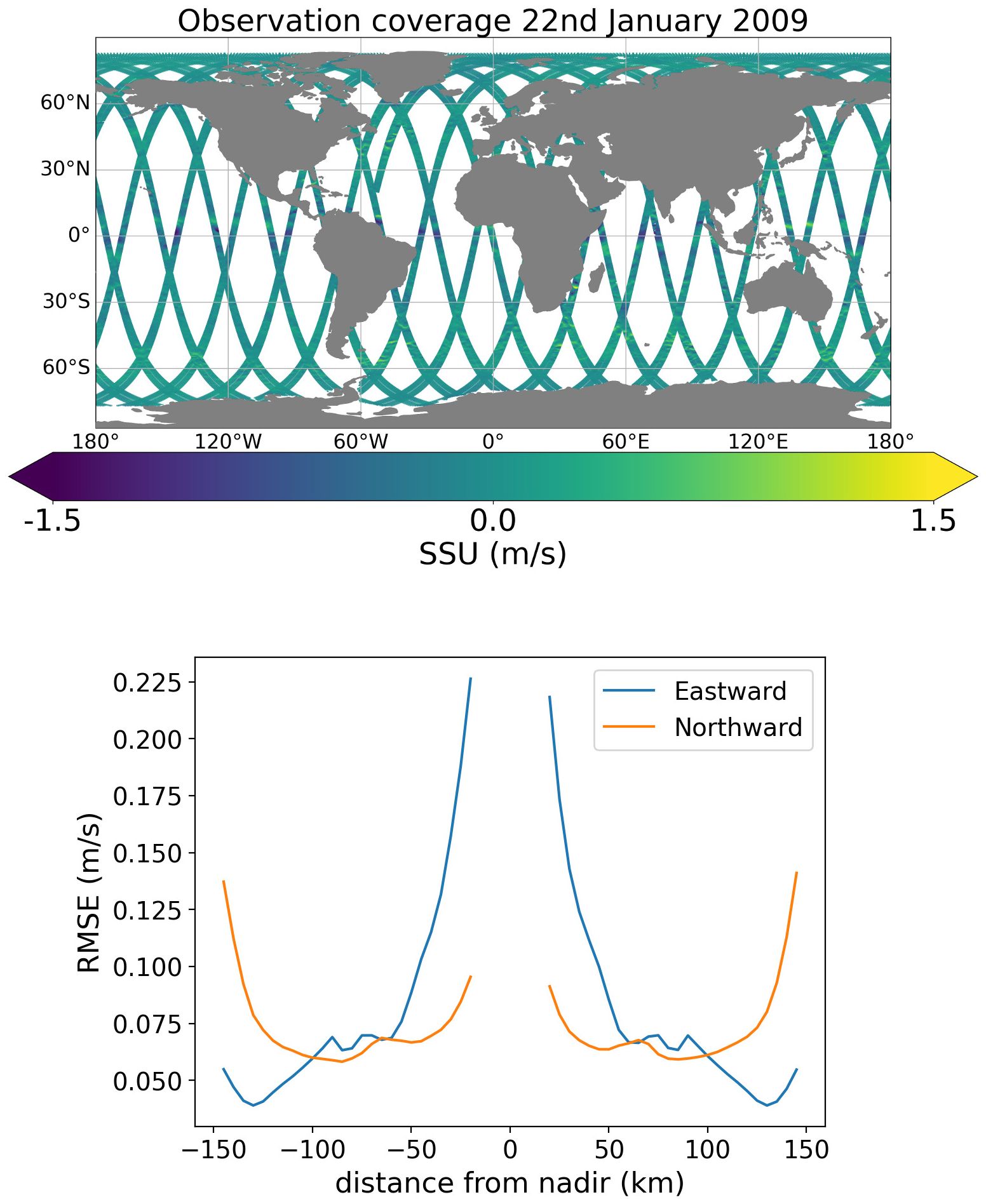
Figure 1 Observation coverage for one day of SKIM data (top) and instrument error structure across the swath (bottom), with the blue line showing the error in the eastward velocity component and the orange line the error in the northward velocity component.

For high density observations, such as swath satellite data, it is important that some observation thinning is applied so that the assimilation does not overfit information from observations with spatially-correlated errors (Ochotta et al., 2005). In the experiments presented here a simple thinning of 20 km was used in both the across- and along-track directions. This thinning was chosen to be the same as the length-scale applied in the OI used in the observation processing. By thinning at this scale we hope to remove the majority of the spatial correlations in the mapping error. This practically means that only 1/16 of the observations were used in the assimilation. In addition, SKIM observations are not assimilated in regions where sea ice is present.

2.2 FOAM system and assimilation of TSCV data

The FOAM system (Aguiar et al., 2023) used here consists of the NEMO 3.6 ocean model on a global 1/4° tripolar grid with 75 vertical levels (the top model level is 1 m thick), coupled to the CICE sea-ice model (Hunke et al., 2015) and the 3D-VAR data assimilation scheme NEMOVAR (Waters et al., 2015). NEMOVAR is a multivariate, first-guess-at-appropriate-time (FGAT), incremental variational data assimilation scheme developed specifically for NEMO. The state vector consists of temperature, salinity, SSH, zonal and meridional velocity and sea ice concentration. The scheme uses multivariate balance relationships to allow correlations between different variables in the background error covariance (Weaver et al., 2005). With the exception of temperature, which is defined as the lead variable, variables are separated into balanced and unbalanced components, and the control vector consists of temperature and the unbalanced salinity, SSH and velocity components. Water mass conservation properties are used to define the salinity balance, hydrostatic balance is used for the SSH balance and geostrophy is used for the velocity balance. Note that sea ice concentration is treated separately (no updates are made to ocean variables based on changes to the SIC and vice versa). The spatial background error correlations in NEMOVAR are modelled using an implicit diffusion operator (Mirouze et al., 2016).

FOAM uses a 24-hour assimilation window and the daily increments produced by NEMOVAR are applied during a 24-hour model run using IAU (incremental analysis update; Bloom et al., 1996). As velocity observations are not assimilated in the standard FOAM configuration, the only adjustments to the velocities (when no velocity observations are available) are made through the geostrophic balance. The geostrophic balance is only applied outside of the equatorial region, so no corrections are made to velocities close to the equator unless velocity observations are assimilated.

Two altimeter bias correction terms are included in the assimilation system used operationally in FOAM. The first altimeter bias term is designed to correct for errors in the Mean Dynamic Topography (MDT) which is used to relate observed SLA to the model SSH (Lea et al., 2008). While we don’t use an MDT in the OSSEs here, the synthetic altimeter observations do include an error associated with the different mean SSH in the NR compared to the mean SSH of the lower resolution system used in the OSSEs, so we retain this bias correction term. The second altimeter bias term is designed to account for differences in the model and observed SLA due to the Dynamic Atmosphere Correction (DAC) which is generally applied to altimeter data and has a large impact at high latitudes. In our OSSE framework, the synthetic observations do not include DAC, however, we retain the bias correction term to account for biases associated with different resolved processes in the NR and OSSEs at higher latitudes.

We specify the background error covariances in NEMOVAR by defining a field of background error standard deviations and background error correlation length-scales for each assimilated variable. We specify spatially and seasonally varying background error standard deviations at the surface for temperature, unbalanced salinity, unbalanced SSH and sea ice concentration, and flow-dependent parameterisations for the sub-surface error standard deviations for the 3D variables. For temperature and unbalanced salinity, a combination of two length-scales is used for the horizontal background error correlations and the vertical background error correlations are based on the local mixed-layer depth in the background field. The unbalanced SSH error correlation length scales are specified as 400 km and the sea ice concentration error correlation length scales are specified as 25 km. The observation errors in NEMOVAR contain no spatial correlations and observation error standard deviations for the standard observation types are spatially and seasonally varying.

As the standard FOAM system does not assimilate velocity data, some developments were required to allow for the assimilation of TSCV data for this study. These were updates to include velocities in the observation operator, the specification of surface observation error standard deviations and the specification of velocity background error covariances. In the following subsections we provide a description of the estimation of the velocity observation and background error covariances.

2.2.1 TSCV observation error specification

We need to specify observation errors for the surface zonal and meridional velocities to be used in the assimilation of the TSCV data. The observation errors required by the data assimilation system include the measurement errors (including the mapping and, where appropriate, the instrument errors shown in Figure 1) as well as the representation errors which describe the mis-match in the resolution represented by the observations and the model, as well as processes missing from the model (Janjić et al., 2018). The mapping error in these experiments is approximately 2.5 cm/s, estimated from a subsample of the TSCV observation data. For the OSSEs presented here the observations are generated from outputs of a higher resolution model run so the representation error should be the differences in the 1/12° NR model’s representation of the ocean compared to the ¼° model used in the OSSEs. We calculated the representation error by comparing the variability in the FOAM ¼° and the 1/12° NR daily mean surface velocities. The day-to-day variability in the surface velocity was calculated for both ¼° and the 1/12° runs over one year at each grid-point and a global offset was determined. This offset of approximately 7 cm/s is assumed to be an approximation to the global average representation error. However, the representation errors are likely to be spatially varying with larger errors in more energetic and variable regions. To allow for spatial variability in our estimate, the annual 1/12° 2D surface velocity variability field was interpolated to the ¼° grid, smoothed using a Gaussian filter with 1.5° length-scale and then normalised by the 7 cm/s offset to produce a 2D field of the representation error. Smoothing of the representation errors is necessary to ensure that they don’t vary too quickly over the scales of the background error correlations. The representation errors are largest in the equatorial region, the western boundary currents and other regions of high variability (see Supplementary Figure 1).

2.2.2 Velocity background errors

For the assimilation of TSCV data, new background error standard deviations and length-scales are required for the unbalanced components of zonal and meridional velocities. The velocity balance in NEMOVAR is geostrophic so the unbalanced component represents the ageostrophic velocity component. The magnitude of the unbalanced velocity background errors will determine how much of the signal in the observations is used to correct the ageostrophic velocity and how much is used to correct the geostrophic velocity. We have used the NMC method (Parrish and Derber, 1992) to estimate the forecast error covariances. This method uses the difference between 48-hour and 24-hour forecast fields, valid at the same time, as a proxy for the forecast error. To produce an estimate of unbalanced velocity error covariances we applied the inverse of the NEMOVAR balance operator to the forecast difference fields to remove the balanced (geostrophic) component prior to the NMC calculation.

For calculating the surface background error standard deviations and horizontal correlation scales, the NMC method was applied to the (unbalanced) surface zonal and meridional velocities from a previous two-year run of the ¼° FOAM system. We applied a function fitting to the estimated NMC error covariances to determine two horizontal correlation length-scales at each grid point and the surface background error standard deviations associated with these (i.e. the respective weighting of these correlation length scales). A final step was to scale the total background error standard deviations to be consistent with the global observation-minus-background RMSE for surface zonal and meridional velocity estimated by comparing a control run (which did not assimilate TSCV data) to the simulated TSCV observation data. In the resulting covariance estimates (see Supplementary Figure 2) the short length scales vary between around 40km at high latitudes and 150km at the equator, the long length scales vary between 200km in high latitudes and 400km in mid-latitudes. In both the short and long length scales, the shortest scales are seen in the highly variable regions of the western boundary currents and the ACC (Antarctic Circumpolar Current). The surface background error standard deviations are highest in the region of the equatorial currents and in the western boundary currents and ACC.

The parameterization used to represent the temperature and salinity vertical background error correlations in FOAM sets the vertical length-scales at the surface equal to the mixed layer depth (based on the Kara et al., 2003 definition) in the background model field on each cycle (see Waters et al., 2015 for more details). We use a similar parameterization for zonal and meridional unbalanced velocity vertical length-scales but choose a different definition of mixed layer depth (MLD001, which is the shallowest depth where the density increases by 0.01 kgm-3 relative to the 10m density). The NMC error covariances for the full 3D unbalanced velocity fields were calculated for a single month, December, and the vertical background error correlations with the surface were compared to the monthly average Kara mixed layer depth and MLD001 (see Supplementary Figure 3). The Kara mixed layer depth was found to be deeper than the NMC scales would suggest, while MLD001 provided a good approximation to the vertical correlation length-scales at the surface.

The NMC background error standard deviations reduce with depth. We therefore use the tapering function shown in Equations 1, 2 to parameterize the subsurface unbalanced velocity standard deviations. This is similar to the function used to taper salinity background error standard deviations in NEMOVAR, but has been tuned to be consistent with the 3D NMC velocity error estimates. The parametrized background error standard deviations at each model grid point at each time are specified by:

$\begin{array}{ll}f(z)=0.05+0.95(1-tanh[ln\frac{z}{L}])/2.& (1)\end{array}$

$\begin{array}{ll}\sigma (z)=\sigma (0)f(z)& (2)\end{array}$

where σ(z) is the background error standard deviation at each grid point and time, z is depth and σ(0) is the surface background error standard deviations estimated from the NMC estimates, as described earlier. L is the length scale for the tapering function and varies at each grid point and time. It is set equal to MLD001 away from the equator and is ramped up to 150 m at the equator to capture the larger background error standard deviations with depth in the tropics seen in the 3D NMC estimates. A comparison between the NMC estimates and parameterised background error standard deviations is provided in Supplementary Figure 4.

2.2.3 Initialising near-inertial oscillations

Single observation experiments were performed to determine how the model responds to balanced and unbalanced velocity increments. Figure 2 shows the results for a single idealised velocity innovation (0.5 m/s in the Eastward direction, 0.5 m/s in the Northward direction) in the middle of the South Atlantic. This innovation was fed into NEMOVAR and the resulting balanced/unbalanced increments are shown. The balanced increments have smaller magnitude and spread than the total increments, and the total increments are more isotropic in their structure. However, when the increment was included in the model during a 24-hour IAU step, the model response to the balanced and total increments in Figure 2 is very similar and looks largely like the structure and magnitude of the balanced increments. This suggests that the unbalanced component of the increments is not being retained by the model.

Figure 2

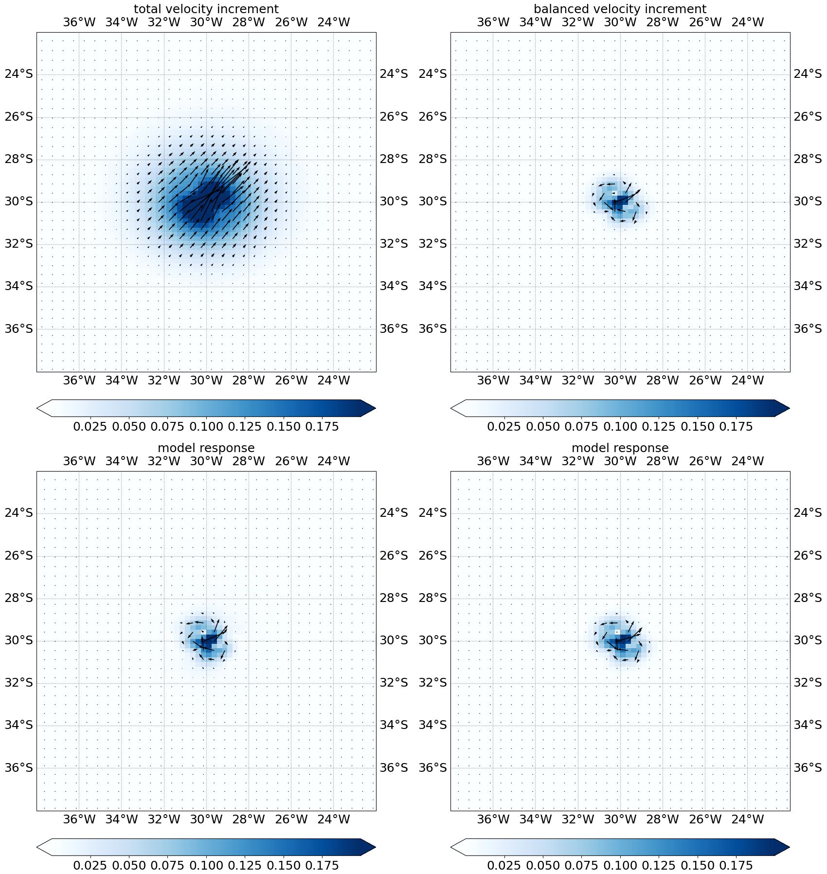
Figure 2 The top plots show the total velocity increment in m/s (left) and balanced/geostrophic velocity increment in m/s (right) for an idealised single TSCV observation. The bottom plots show the model response in m/s to the total (left) and balanced (right) increments at the end of a 24 hour IAU step.

One reason for this is the way the increments are applied to the model during the IAU. Away from the equator and coasts, Near-Inertial Oscillations (NIO) are a large component of the ageostrophic (unbalanced) velocities. NIOs are rotations of the near surface velocity at the inertial period T=2π/f, normally caused by localised wind changes. In the Northern Hemisphere these rotations are clockwise and in the Southern Hemisphere they are anti-clockwise. During the IAU step, we nudge velocity increments into the model. In regions where NIOs dominate, the model responds to the unbalanced velocity perturbations in a similar way that it would respond to a perturbation in the winds, i.e. it rotates the perturbation at the inertial period. This effect is demonstrated in Figure 3 in the Mid-South Atlantic (the same location as the single observation shown earlier). In the top plot, an unbalanced velocity increment is applied with direct insertion. Direct insertion is where the full increment (green arrow) is applied at zero hours (the start of the day). The increment at zero hours is derived from the increment at 12 hours (cyan arrow) by rotating the increment by the inertial period. The blue arrows show how the model responds. We can clearly see that the model velocities begin to rotate anti-clockwise with a period of approximately 24 hours (the inertial period at this latitude). The middle plot shows how the model responds when the same unbalanced velocity increment is applied using IAU (this is how increments for other variables are applied in the FOAM system). In this case, the North Easterly increment is nudged in evenly throughout the first 24 hours. The model responds to the perturbation with a rotation (similar to the bottom plot), however, at each subsequent time step we force in a new North Easterly correction which partially cancels the model rotation. This results in a much smaller model response compared to the direct insertion case by the end of the IAU.

Figure 3

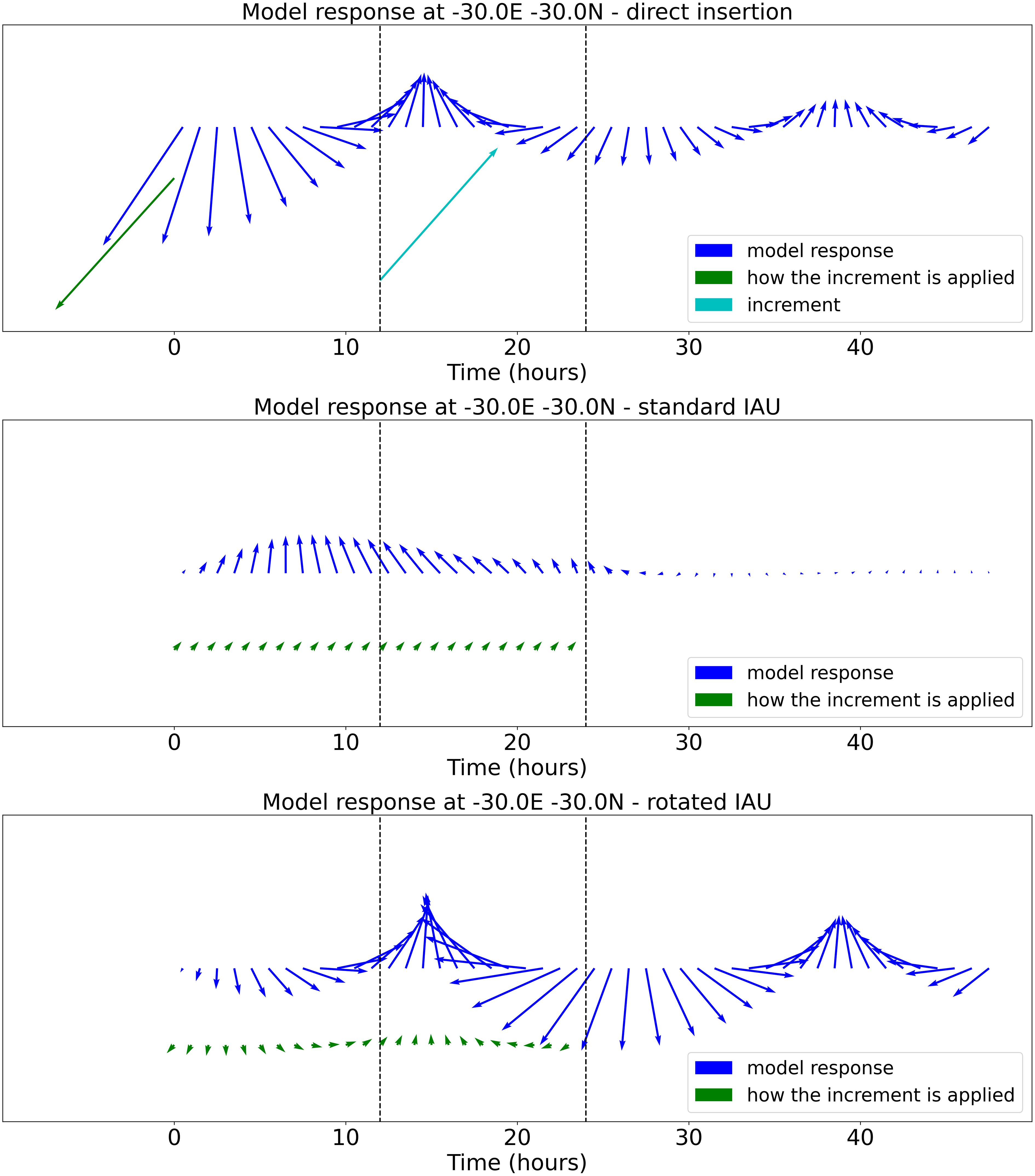
Figure 3 The blue arrows show the model’s response to a North East unbalanced velocity increment valid at 12 hours (shown by the cyan arrow in the top plot). The green arrows show how the increment is applied to the model. In the top plot, the increment is rotated by the inertial period to 0 hours and applied using direct insertion. In the middle plot, the velocity increment is applied with the standard IAU over the first 24. In the bottom plot, the velocity increment is applied with a rotated IAU over the first 24 hours. The arrows are plotted using the same scaling.

We now assume that the unbalanced component of the velocity increment is largely due to errors in the NIOs. Rather than applying the unbalanced velocity increment in a standard IAU which dampens any NIO as just described, we propose a scheme which attempts to initialise the NIOs using a rotated IAU. The velocity increments are still nudged in throughout a 24-hour window, but the applied increment is rotated by the inertial period at each time step. The bottom plot in Figure 3 shows the model response to this rotated IAU. The model responds with a rotation which looks similar to the direct insertion plot; however, the magnitude of the model response is smaller in the IAU (first 24 hours) and slightly larger in the forecast (24-48 hours). Using an IAU is considered preferable to direct insertion as it reduces shocks to the model so this rotated IAU method will be tested for improving the initialisation of NIO in the experiments described later.

The above description describes the initialisation of NIOs using the unbalanced increments in an idealised single observation experiment. In the full assimilative system, we have numerous TSCV observations valid at different times in a single assimilation cycle. To initialise the NIOs using the method described in the previous paragraph, we need to know the time that the increments are valid for. Ideally, we would use a 4D-VAR approach to assimilate the velocity data at the correct time, but this is not currently practical within our system. Instead we create a field of increment times on the model grid by using the time from the nearest TSCV observation on each assimilation cycle. These increment times are then used to rotate the applied unbalanced increments in the IAU. To avoid ambiguity in the increment times, we remove any crossing satellite tracks within the assimilation window. We do this by only using the descending TSCV tracks (ascending tracks are discarded) and removing observations poleward of 60° N/S. Figure 4 shows an example of the observation times for a single day (top plot) and the corresponding increment-time field (bottom plot). Note that in our application of this method the balanced (geostrophic) increments are applied using a standard IAU (no rotation) and the full unbalanced increments are applied with the rotated IAU (i.e we assume that all the unbalanced corrections are due to errors in the NIOs).

Figure 4

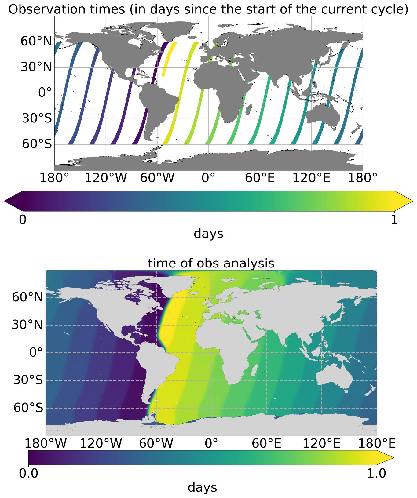
Figure 4 Time of day of the descending TSCV observations in the top plot and the resulting times of the increments (on the model grid) in the bottom plot.

2.3 Experiment description

The main OSSEs are summarised in Table 1. The Control experiment is the baseline experiment which only assimilates simulated observations for the standard observation types (SST, temperature and salinity profiles, SSH, SIC). The A-TSCV experiments use an identical set-up to the control, but in addition to assimilating the standard observation types, they assimilate the simulated TSCV observations described in section 2.1.2.2. Two A-TSCV experiments are run for the full control period: one where the TSCV observations only contain the mapping error (A-TSCV_No_Err in row 2) and one where the TSCV observations include both the mapping error and instrument error (A-TSCV_Instr_Err in row 3). In addition, two short experiments are run to assess the impact of initializing the NIOs, one using the standard IAU (A-TSCV_No_NIO_corr in row 4) and one using the rotated IAU (A-TSCV_NIO_corr in row 5).

Table 1

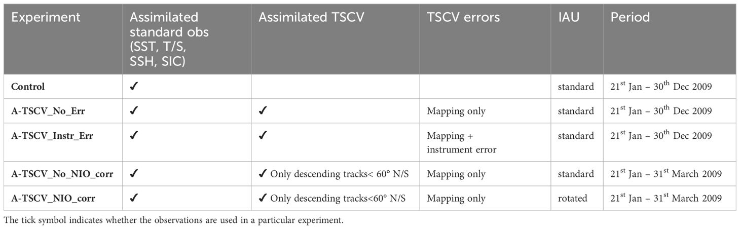
Table 1 Summary of OSSE experiments.

A spin-up run starting from the 1^st of January 2009 and assimilating the control observations was performed. The run was started using ocean/ice restarts from the 1^st of January 2009 from the AtlantOS control (Mao et al., 2020), the altimeter bias terms were initialised as zero. The main runs were then all started from the same spin-up run on the 21^st of January 2009, in the A-TSCV experiments TSCV data were assimilated from this date. The main experiments were run until the end of 2009 with the main assessments carried out from the 25^th February 2009 which allowed for a spin up with TSCV assimilation of more than a month. Seven-day forecasts were run every 7 days throughout the period.

The OSSEs are designed to differ from the NR by using different surface forcing, a different resolution model and different initial conditions to realistically represent the differences in our forecasting systems and the real ocean. While both systems use the NEMO ocean model, they are run at different NEMO versions and include some differences in the parameterisations, for example different lateral eddy diffusivity and horizontal bilaplacian eddy viscosity values (Mao et al., 2020) and the NR included a large scale correction for precipitation (Gasparin et al., 2019) which was not in the model used in the OSSEs. The OSSEs are run at ¼° resolution compared with the 1/12° resolution of the NR and the OSSEs are forced with ERA5 fluxes (Hersbach et al., 2020) with a 100% wind/current coupling coefficient. The fluxes differ from the near-real time operational ECMWF fluxes used to drive the NR (Shihora et al., 2022 give an example of the differences in surface pressure from ERA5 compared to operational ECMWF forcing). When comparing the daily mean 10m wind speed between the near-real time operational ECMWF and ERA5 fluxes, in many regions the percentage difference exceeds 25% (not shown). The surface velocity global RMSE of the control relative to the NR are 13/12 cm/s for zonal/meridional velocity. These global errors are broadly comparable with the assessment of near surface velocities from the global ¼° FOAM system using drifter-derived velocities in Aijaz et al. (2023), which found near surface RMSEs between 13 and 16 cm/s. This supports the realism of the OSSE design.

3 Results

In sections 3.1-3.3 we assess the results from A-TSCV_No_Err and A-TSCV_Instr_err while in section 3.4 we assess the impact of correcting the NIO with the TSCV assimilation.

3.1 Global results

Figure 5 shows the impact of assimilating TSCV data on global analysis RMSE as a function of depth/time. Statistics are calculated with respect to the NR on a common ¼ degree grid. The surface velocity RMSEs are reduced by approximately 23% in the A-TSCV_Instr_Err experiment and approximately 26% in the A-TSCV_No_Err experiment. The improvements to velocity with TSCV assimilation is largest at the surface, but there are improvements throughout the water column and these are larger in the A-TSCV_No_Err experiment. Temperature RMSEs are also improved below 300 m in A-TSCV_Instr_Err and throughout the water column in A-TSCV_No_Err, but there is little change to global salinity RMSEs. The SSH results show a significant improvement with TSCV assimilation of more than 0.5 cm (approximately 14%) to the global SSH RMSE.

Figure 5

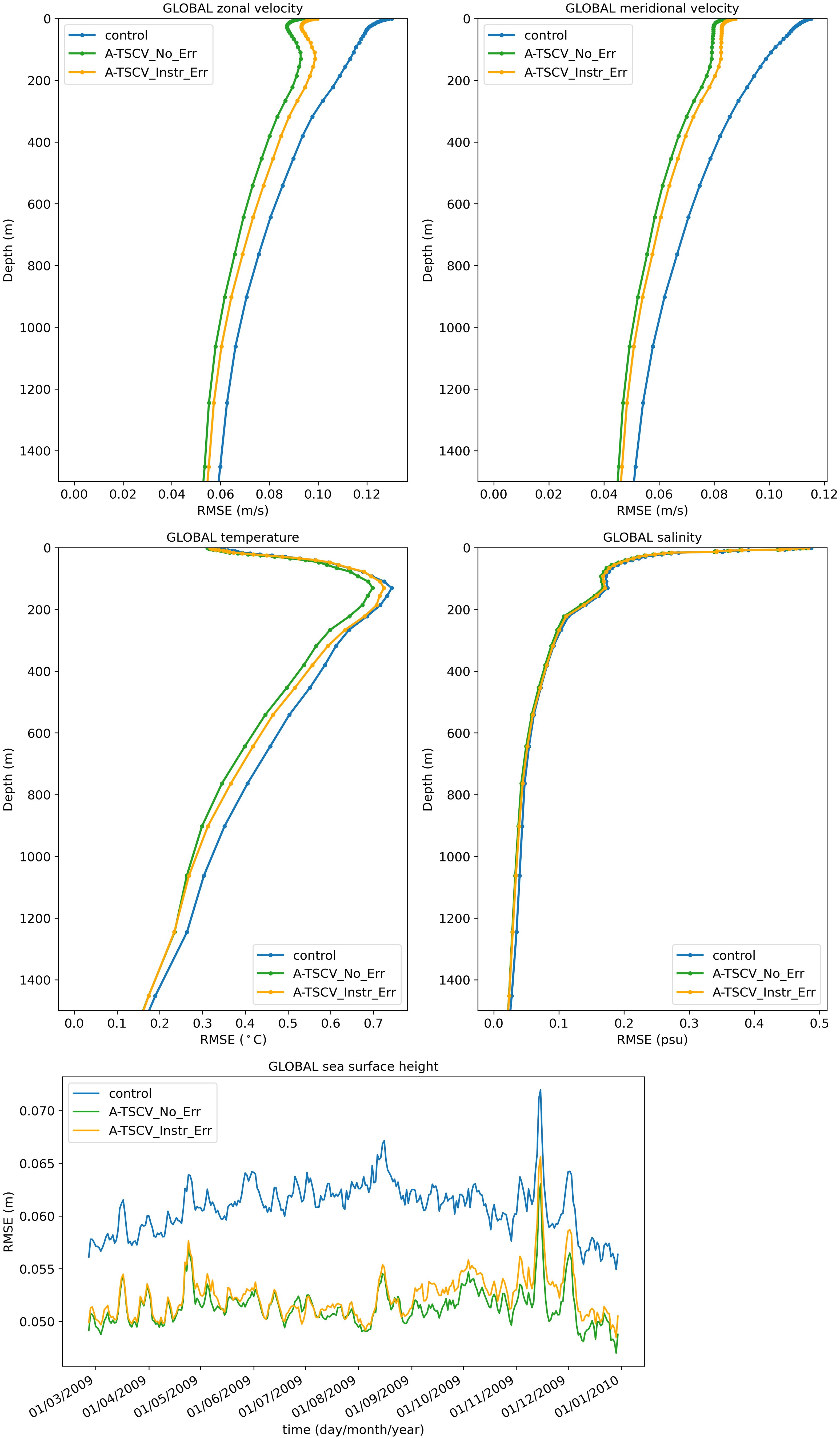
Figure 5 Global RMSE calculated over 25/02/2009 – 30/12/2009 for zonal velocity (top left), meridional velocity (top right), temperature (middle left), salinity (middle right) and SSH (bottom).

Figures 6 show the spatial difference in the RMSE between the A-TSCV_Instr_Err experiment and the control for July at the surface and 220m. Throughout this paper, blue indicates regions where the A-TSCV_Instr_Err experiment has a smaller RMSE than the control, while red indicates regions where the RMSE is larger than in the control. Significant reductions to surface velocity RMSE are seen in the equatorial region, the western boundary currents (WBC) and the Antarctic Circumpolar Current (ACC). The results show some small degradations to zonal surface velocities in the middle of the gyres. However, a similar degradation is not seen when assimilating the TSCV data without instrument error (see Supplementary Figure 5). This may suggest that the background and observation errors require further tuning to optimise the impact of the TSCV assimilation when realistic observation errors are present. At 220 m there are some small improvements to velocity RMSE along the equator and in the WBC and more significant improvements in the ACC. Regional results in the next section provide more detail on the improvement with depth in these regions. There are also some regions with degradations. These predominantly occur in the tropics, away from the equator but close to the coast. The dynamical balances prescribed in NEMOVAR to spread information between variables and in the vertical are not dynamically consistent in regions with complex vertical density structures. In general, the degraded areas appear to be tropical regions which have large freshwater input from rivers and are likely to have complex vertical salinity structures which distort the vertical propagation of the increments. For both SST and SSH, RMSEs are improved primarily in the WBCs and ACC. There are also some improvements to SSTs in the region of the tropical instability waves in the East Tropical Pacific and some degradations in the regions where the 220m velocities are degraded.

Figure 6

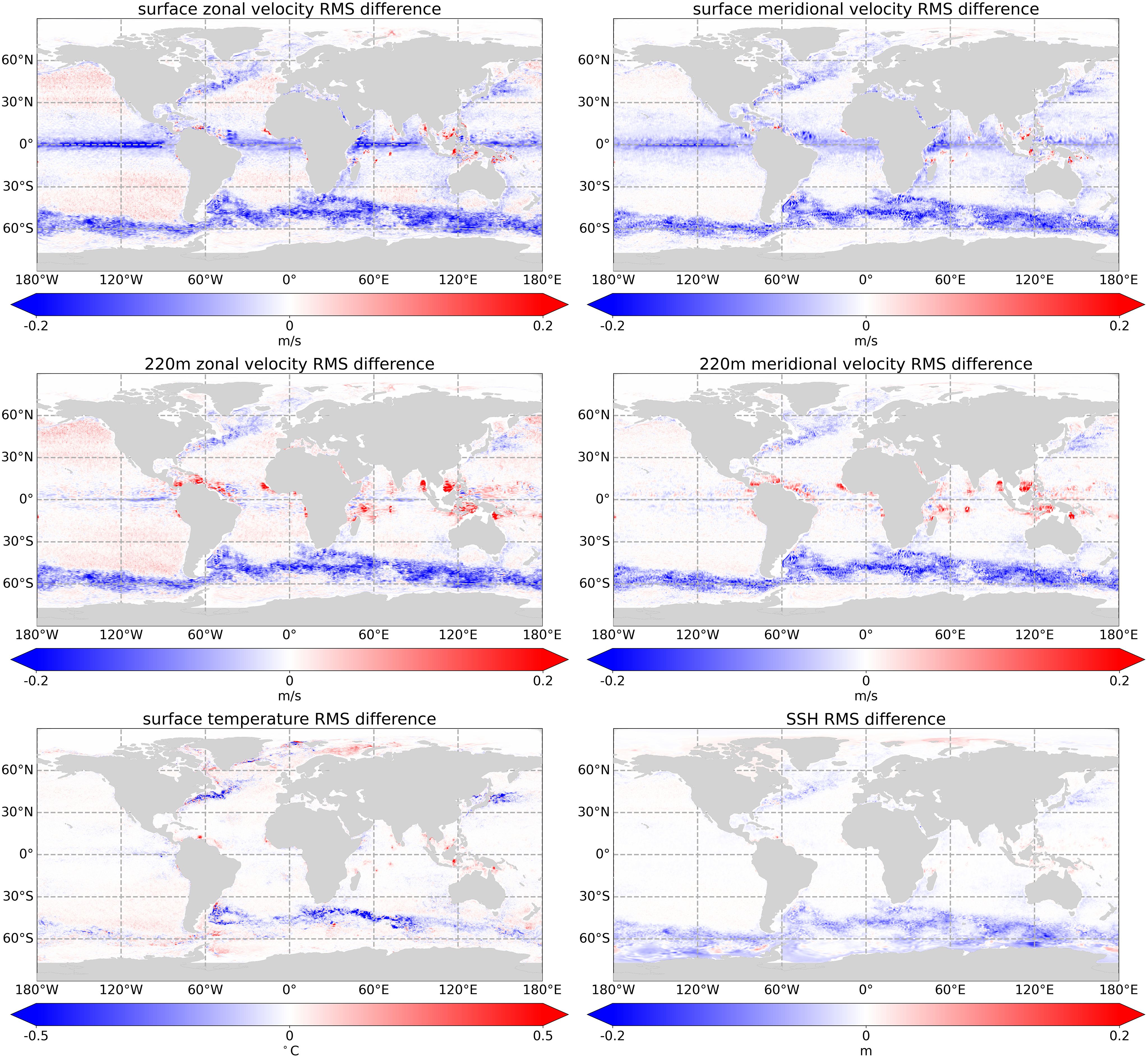
Figure 6 Spatial plot of A-TSCV_Instr_Err RMSE minus control RMSE calculated between the 25^{t h} of February and 30^th of December for surface zonal velocity (top left), surface meridional velocity (top right), 220 m zonal velocity (middle left), 220m meridional velocity (middle right), SST (bottom left) and SSH (bottom right). Blue areas indicate regions where the A-TSCV exp has a lower RMSE than the control while red indicates regions where the RMSE is higher.

We produced 7-day forecasts every 7 days for the control and OSSEs. The forecasts are assessed against the Nature Run and in Figure 7 the global surface velocity RMSE is plotted as a function of forecast lead time. The improvement to the surface velocities is well retained throughout the 7-day forecast. In fact, the experiments which assimilate TSCV data with instrument error have a lower zonal velocity RMSE at forecast day 6, and a lower meridional velocity RMSE at forecast day 5 than the control has at forecast day 1. This implies that we get a 4-day gain in global velocity forecast RMSE accuracy when assimilating TSCV data without instrument error. When instrument error is not included in the TSCV data, there is a 5-day gain in global velocity forecast RMSE accuracy.

Figure 7

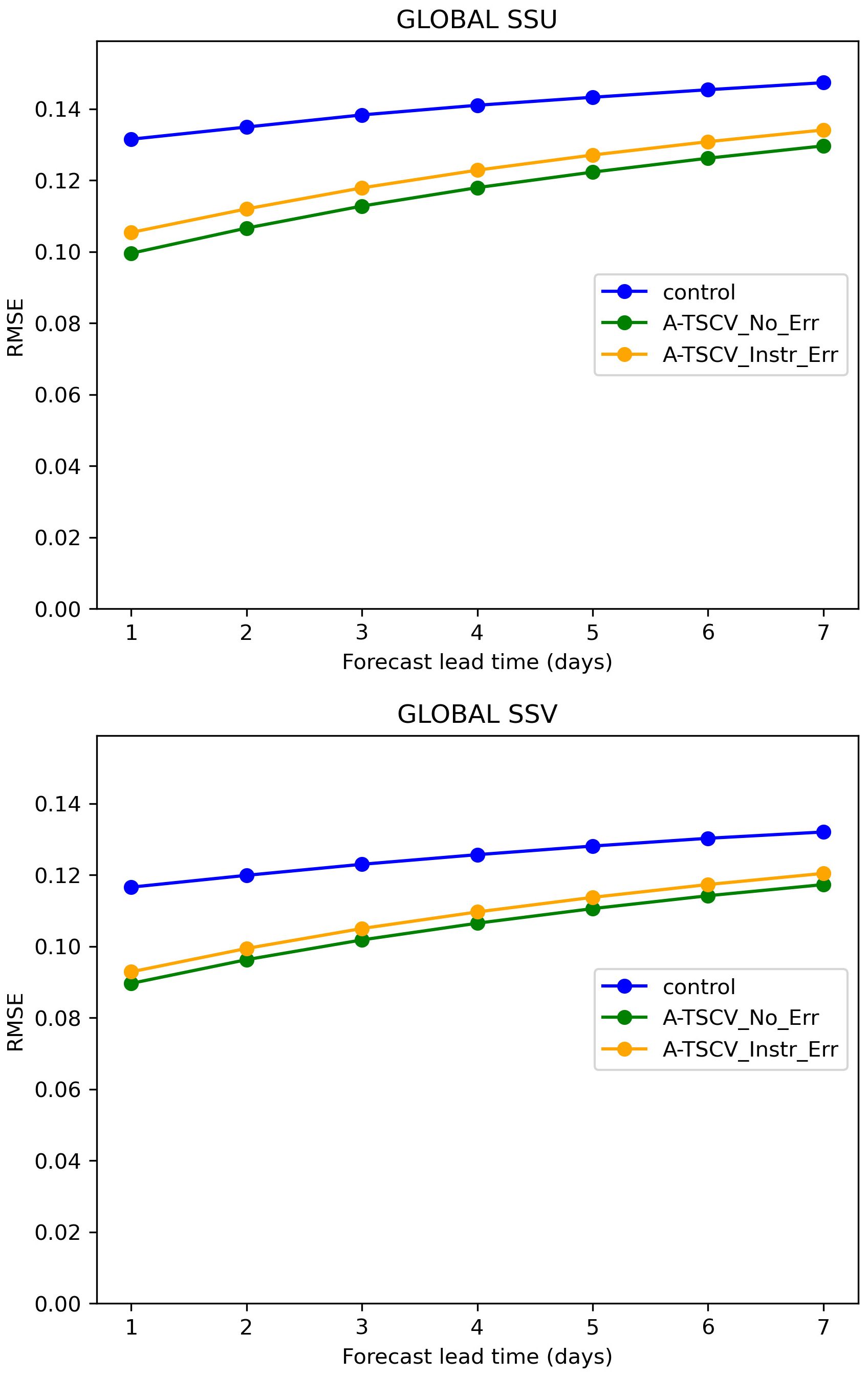
Figure 7 Global forecast RMSE for surface zonal (top) and meridional (bottom) velocity, calculated over 25/02/2009 – 30/12/2009.

3.2 Regional results

In this section we will focus on results from a tropical region and Western Boundary Current (WBC) region. Figure 8 shows the mean surface speeds in July in the NR and the monthly mean errors in the control and A-TSCV_Instr_Err (calculated relative to the NR) for the Tropical Atlantic. There is a good reduction in the errors at the equator in A-TSCV_Instr_Err. In particular, the North Brazil current and northern branch of the South Equatorial Current, which is the Westward current between 0° and 5° North, are improved. This is a region where we would expect the TSCV assimilation to have a significant impact on the predictability of currents. There is no geostrophic balance near the equator, which means that velocities are not constrained in this region by data assimilation in the control experiment.

Figure 8

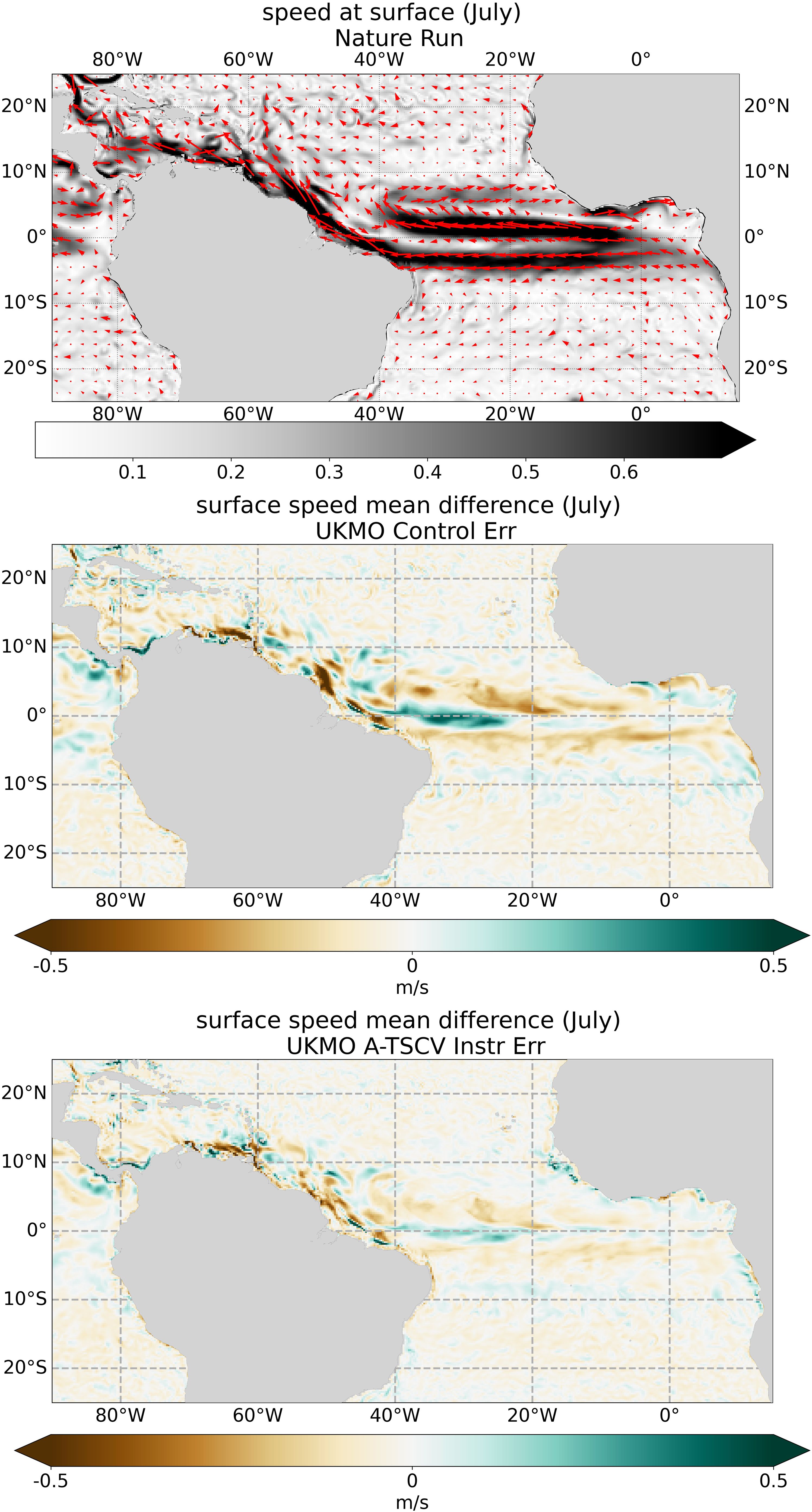
Figure 8 Mean speed at surface in July for the NR (top) and monthly mean error in surface speed for the control (middle) and A-TSCV_Instr_Err (bottom).

The RMSE statistics as a function of depth for the Tropical Atlantic region in Figure 9 provide more of a mixed picture. While there are improvements to velocity RMSE with TSCV assimilation in the top 100 m, there are degradations below that. From Figure 6 we see that the main degradations to the zonal velocity RMSE in the Tropical Atlantic at 220m depth occur away from the equator and primarily in the Amazon outflow region. Similar results are seen in the SST results in Figure 6. These results suggest that degradations in the Amazon outflow region are largely responsible for the degradations to the statistics seen in the Tropical Atlantic results below the surface layers.

Figure 9

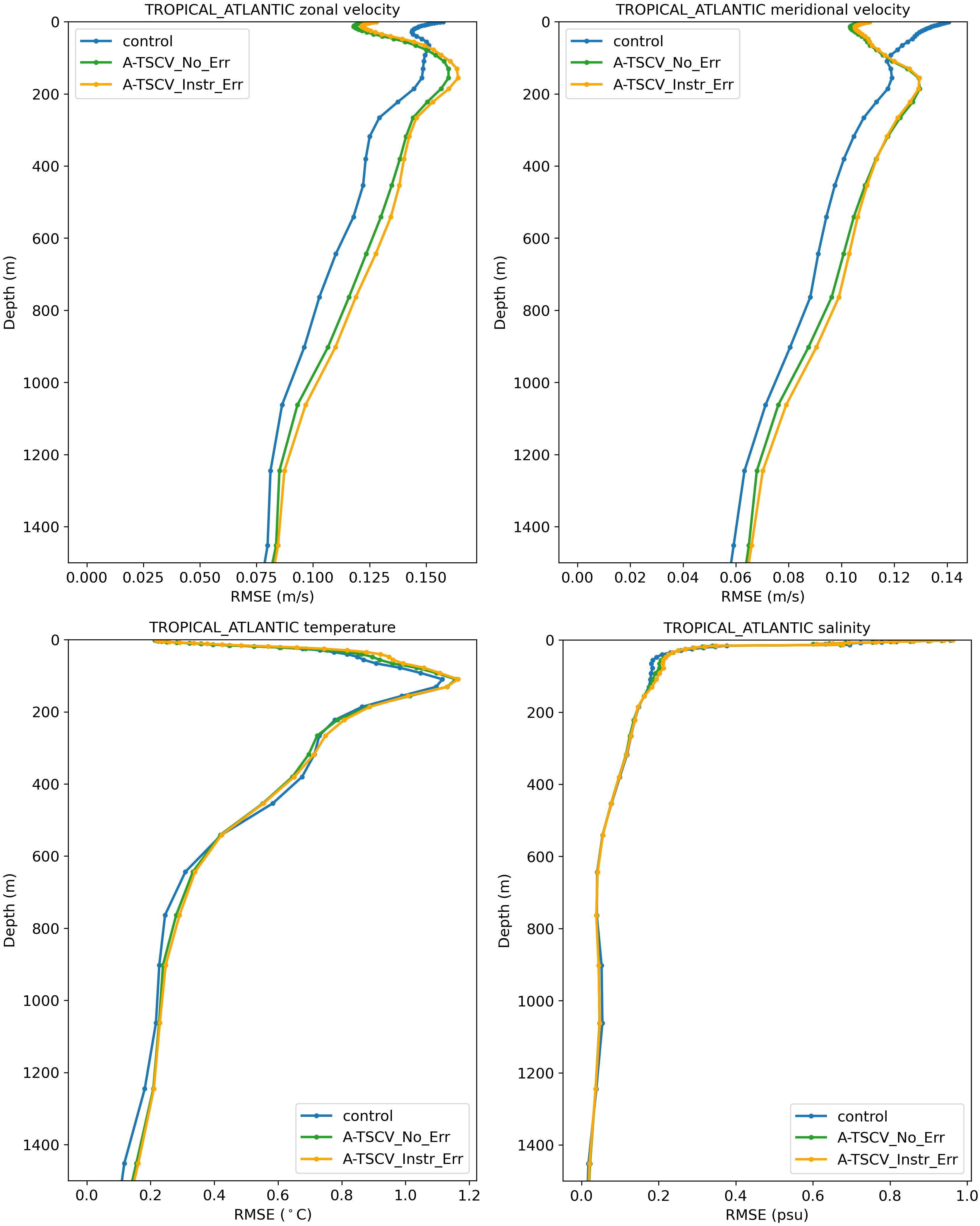
Figure 9 Tropical Atlantic RMSE calculated over 25/02/2009 – 30/12/2009 for zonal velocity (top left), meridional velocity (top right), temperature (bottom left) and salinity (bottom right). The Tropical Atlantic statistics are calculated for region 8 in Figure 6 from Mao et al. (2020).

Figure 10 shows the monthly mean speeds and mean speed errors for the South Atlantic WBC region in July. From the mean error plots, the control significantly underpredicts the strength of the Malvinas/Falkland current. However, this is substantially improved in the A-TSCV_Instr_Err experiment. Altimeter assimilation is unable to correct the Malvinas/Falkland current in part due to the altimeter bias correction scheme. The error in the Malvinas/Falkland current is a persistent, stationary feature in the control experiment and the data assimilation bias correction scheme attributes biases with these temporal and spatial scales to an observation bias in the MDT. Because the data assimilation scheme sees this error as an observation bias, it does not attempt to correct this feature with SSH assimilation. A similar behaviour has been observed in the FOAM system when using real observations, where model biases are aliased in to the MDT altimeter bias term. The assimilation of TSCV data compliments the altimeter assimilation by significantly improving the correction to currents (and SSH) in regions where these features occur. In addition to improving the Malvinas/Falkland current, TSCV assimilation improves the region around the ACC, Drakes Passage and Zapiola rise (a subsurface plateau at 45° W, 44° S with a strong anticyclonic circulation around it, Saraceno et al, 2009).

Figure 10

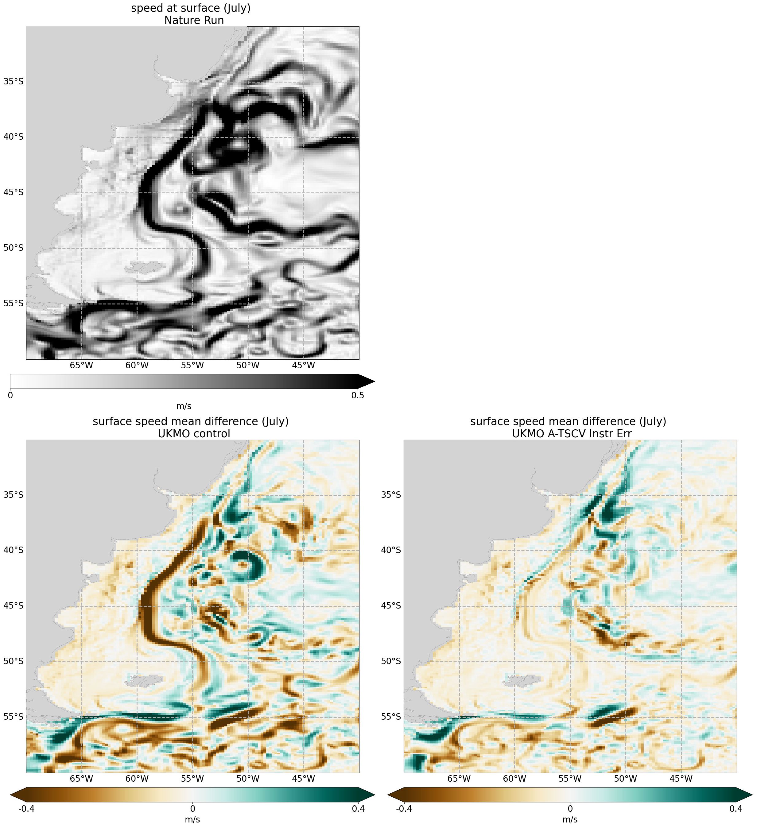
Figure 10 July monthly mean current speed at the surface for NR (top left) and monthly mean error in the control (bottom left) and A-TSCV_Instr_Err (bottom right).

The RMSE statistics for the South Atlantic WBC region are shown in Figure 11. There are improvements throughout the water column for velocity with a reduction to the RMSE of around 27% at the surface and 20% below 1500 m. The improvements at depth (below a few hundred metres) are due only to the correction of the geostrophic velocities. The baroclinic component of the geostrophic velocity correction is applied down to 1500 m – below this depth the improvements are due to the barotropic component of the geostrophic velocity correction. The results from these OSSEs suggest that the TSCV assimilation is able to make significant corrections to the barotropic geostrophic velocities in the WBC and ACC regions which lead to improved velocities down to the bottom of the ocean. A good improvement is also seen in the temperature RMSEs, particularly below 100 m depth. There are also improvements to salinity down to 1500 m. The salinity RMSE is reduced by approximately 5% near the surface and by approximately 20% at 1500 m. The SSH RMSEs (not shown) are reduced by more than 1 cm with TSCV assimilation.

Figure 11

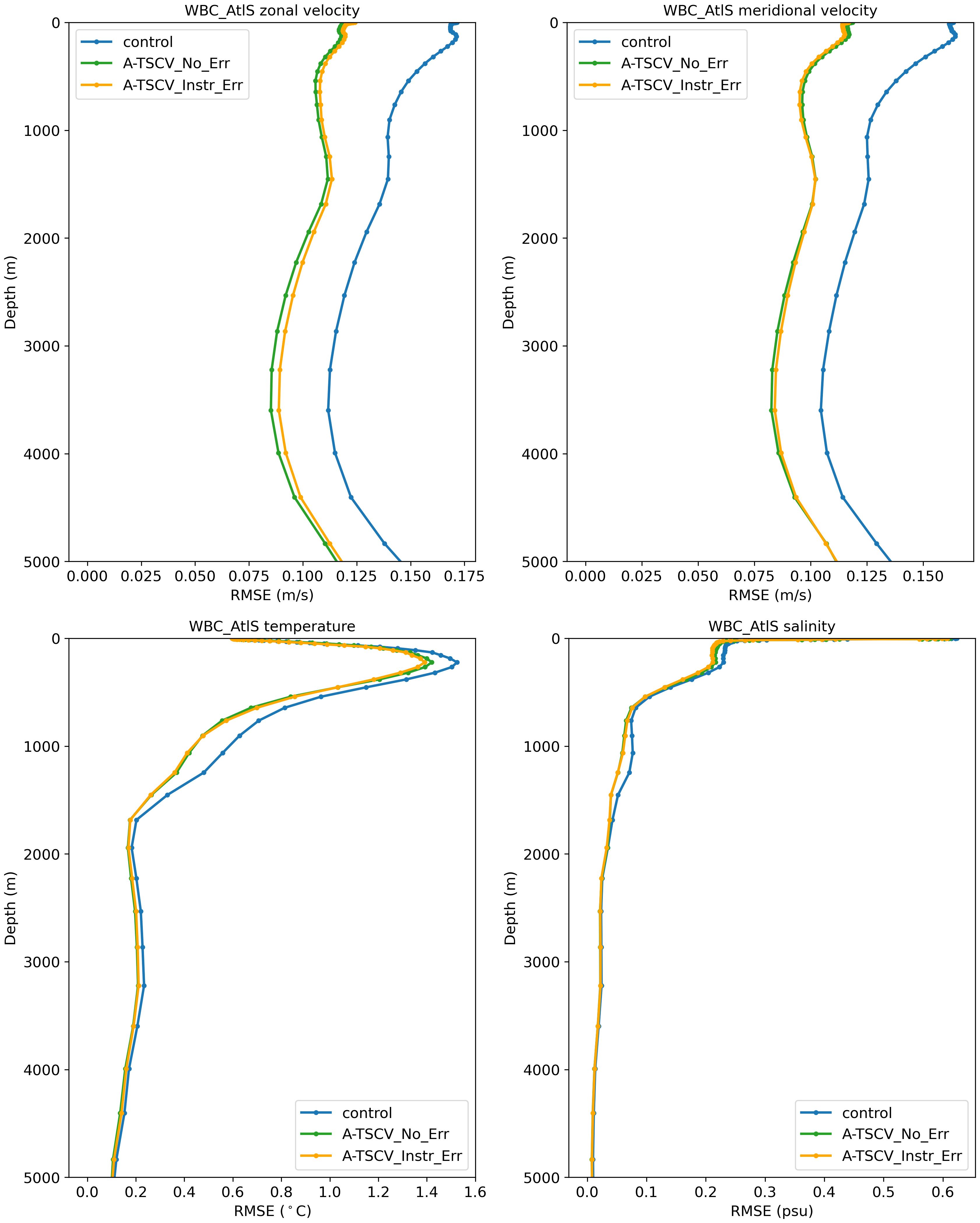
Figure 11 South Atlantic WBC RMSE calculated over 25/02/2009 – 30/12/2009 for zonal velocity (top left), meridional velocity (top right), temperature (bottom left) and salinity (bottom right). The South Atlantic WBC statistics are calculated for region 10 in Figure 6 from Mao et al. (2020).

3.3 Lagrangian assessment

The OceanParcels tool (Delandmeter and van Sebille, 2019) has been used to perform a Lagrangian assessment of the A-TSCV experiments. Particles were seeded globally at a ¼ degree resolution and were propagated for 6 days from the 9^th September 2009 using the model daily analysis velocity fields. The separation of the particles from the NR particles were calculated on each day. Figure 12 shows the percentage of particles within 50 km of the NR particles for 1-6 advection days. The number of particles within 50 km separation after 6 days is increased by 9% in the A-TSCV_Instr_Err experiment relative to the control and there is a 1.5-day gain in prediction accuracy. A 2-day gain in prediction accuracy is seen in the A-TSCV_No_Err experiment. From spatial plots (not shown) the improvement is largely in the equatorial region, WBC and ACC, similar to the results in Figure 6.

Figure 12

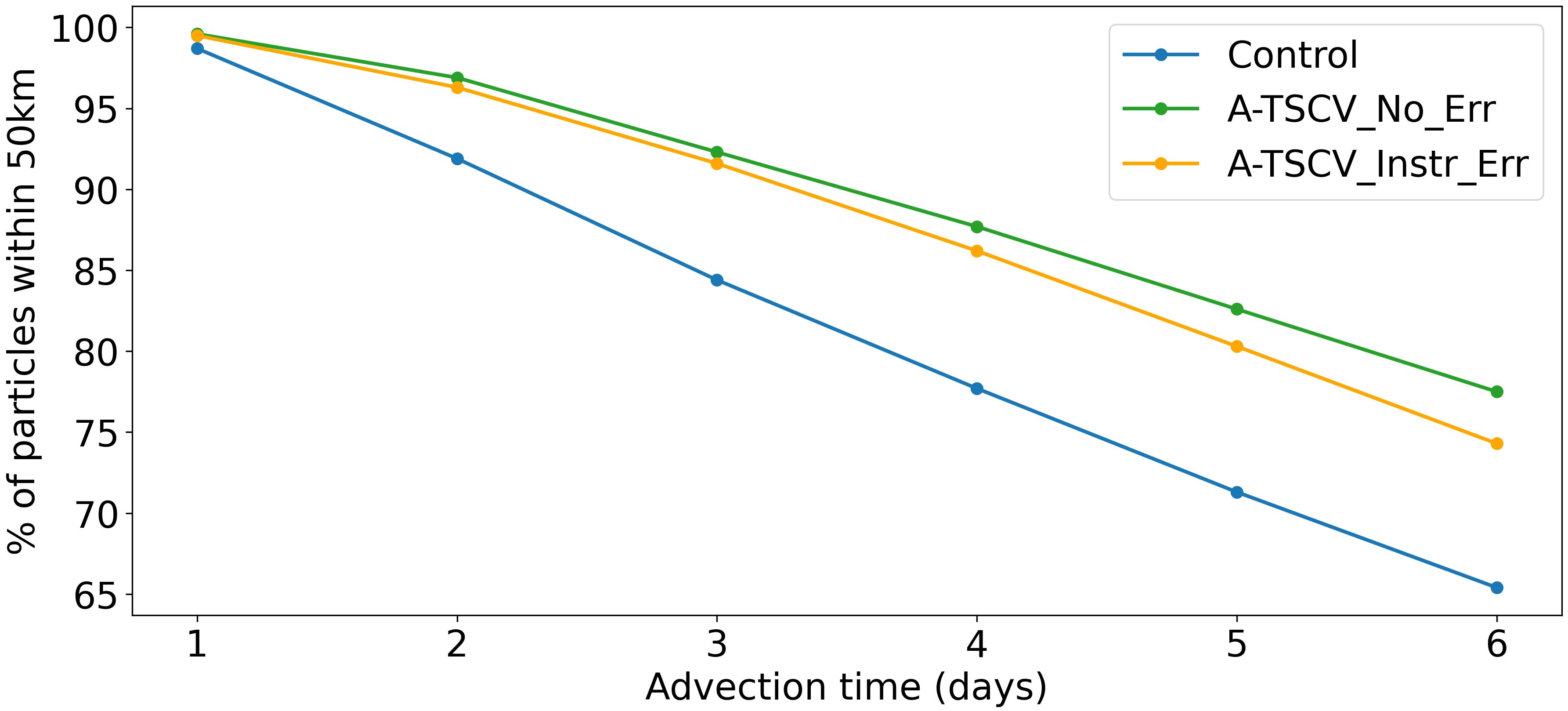
Figure 12 Percentage of particles within 50km of the NR particles for different advection times.

3.4 Near inertial oscillation correction results

In this section we assess the impact of TSCV assimilation on NIOs. In section 2.2.3 we showed that using a standard IAU can lead to a cancelling effect in regions where NIOs dominate. In order to assess the impact of TSCV assimilation on the NIOs in our experiments, we performed a spectral temporal analysis of the clockwise component of the surface velocities in the Northern Hemisphere and counter-clockwise component of the surface velocities in the Southern Hemisphere along latitudinal bands. At each latitudinal band we extracted the spectral power at the inertial period for that latitude. These are plotted as a function of latitude and are shown in Figure 12 (left plots). We see that the behaviour is quite different in the Northern and Southern Hemisphere. In the Southern hemisphere the NR has substantially more power at the inertial frequency than the FOAM experiments which suggests that the NIOs are unpredicted in the FOAM experiments in this region. In the Northern Hemisphere the NR results are more comparable with the FOAM experiments. The free run at ¼° resolution has more power at the inertial frequency than the control run at nearly all latitudes. This implies that data assimilation generally (not just assimilation of TSCV data) leads to a dampening of the NIOs in the model.

When TSCV data are assimilated using the standard IAU (A-TSCV_no_NIO_corr), the spectral power at the inertial frequencies generally increases and is closer to the free run. However, the spectral power at the inertial frequency is significantly larger in the A-TSCV_NIO_corr experiment. This implies that the rotated IAU is able to initialise NIOs through the TSCV assimilation. In the Southern Hemisphere this produces results closer to the NR. However, in the Northern Hemisphere the spectral power at the inertial frequencies over-shoots the NR at some latitudes. The different performance of the rotated IAU in the two hemispheres could be related to seasonal variations in the strength of the NIOs. Spatial assessment (not shown) of the spectral power of the clockwise/anti-clockwise velocity component at the inertial frequency calculate over 10 degree boxes demonstrates that in March 2009, the NR has larger magnitude NIOs in the Southern Hemisphere compared to the Northern Hemisphere. This is consistent with results in D’Asaro (1985). They showed that energy flux to the inertial motion is lower in the presence of a deeper mixed layer depth. In March, while we expect the wind forcing to be strong in the Northern Hemisphere, the mixed layer is deep and this reduces the energy flux to the inertial motion. Interestingly, Watanabe and Hibiya (2002) suggest that the dependence of the energy flux to the inertial motion on mixed layer depth is more important in the Northern Hemisphere, so we may expect to see less of a seasonal cycle in the Southern Hemisphere. These spatial and temporal variations in the strength of the NIOs may also impact the proportion of the ageostrophic velocity increments which can be attributed to NIOs. In future work, the amount of weight given to NIO corrections should be further investigated. The experiments should also be extended to cover a longer period to allow us to assess the impact of the seasonal cycle.

When we compare the RMSE statistics of zonal and meridional surface velocity for March from the A-TSCV_No_NIO_Corr and the A- TSCV_NIO_Corr experiments, we see a negligible impact on results. However, if we focus on the sub-daily variability in the velocity fields we see larger impacts. We calculated a residual surface velocity as hourly surface velocity minus the daily mean surface velocity and then calculated the RMSE of this residual relative to the equivalent values from the NR. Figure 13 (right plots) show the percentage improvement in the residual zonal surface velocity RMSE relative to the control run. In the Southern hemisphere, the A-TSCV_NIO_Corr produces a good improvement to the residual zonal surface velocity RMSE relative to the A-TSCV_no_NIO_Corr and control experiment. The results are more mixed in the Northern Hemisphere, with a small overall degradation. Given that the spectral results suggest a larger under-prediction of the NIOs in the Southern Hemisphere, it is consistent that this is a region where we see improvements in the residual zonal surface velocity RMSE.

Figure 13

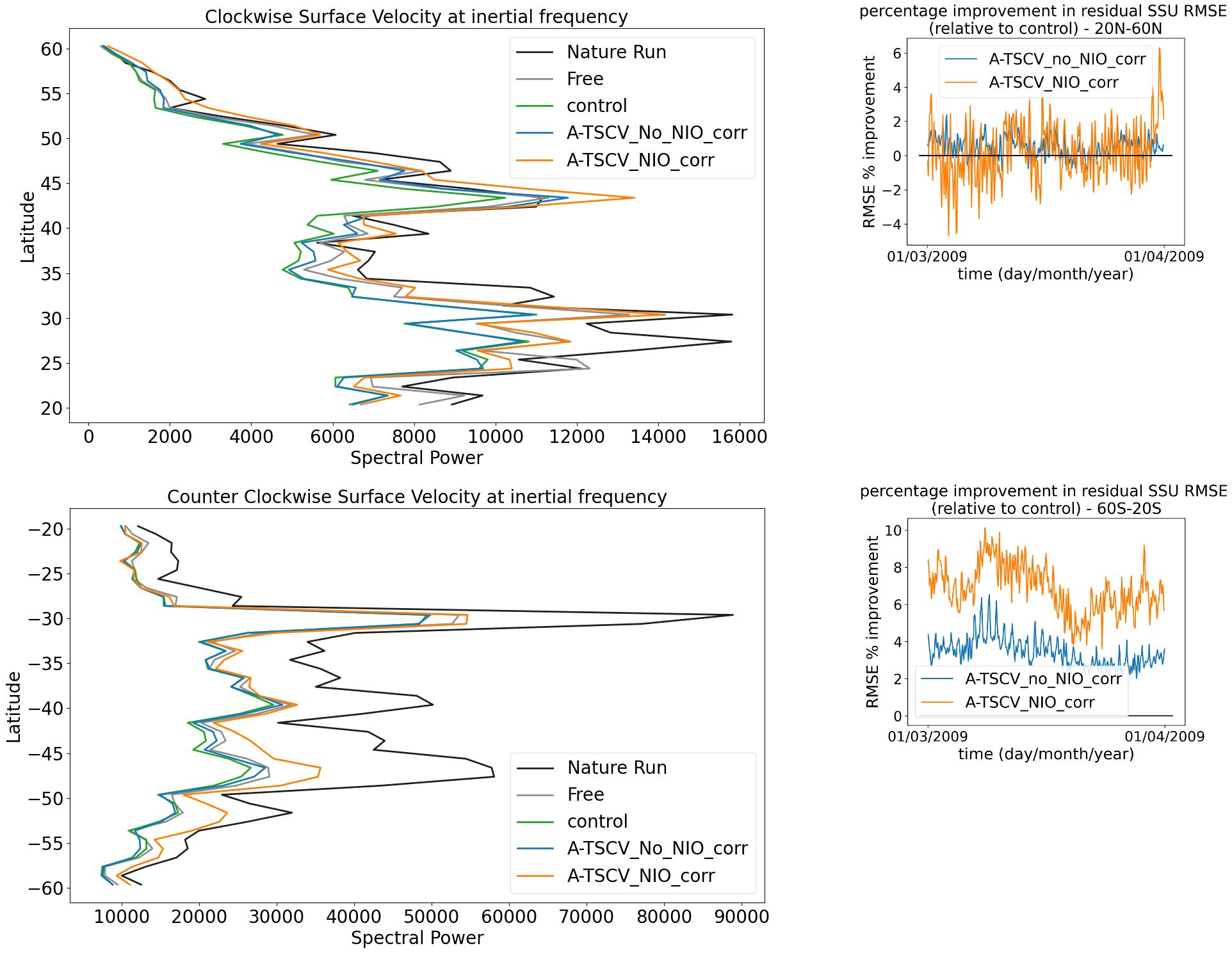
Figure 13 Left plots show the sum of spectral power along latitude bands of the clockwise/counter clockwise component of the surface velocities at the inertial frequency as a function of latitude for March 2009. Top left is the clockwise component in the Northern Hemisphere (20N to 60N), bottom left is the counter-clockwise component in the Southern Hemisphere (20S to 60S). Right plots show the percentage improvement relative to the control of the residual surface zonal velocity RMSE in the Northern Hemisphere (top) and Southern Hemisphere (bottom). The relative surface velocity is calculated from the hourly surface velocity minus the daily mean surface velocity.

4 Discussion and conclusion

In this study we have used OSSEs to assess the potential impact of assimilating satellite TSCV observations in a global ocean forecasting system. The assimilation of synthetic TSCV data in this framework was shown to significantly improve the prediction of surface currents with a reduction in the analysis RMSE of approximately 23%. This improvement was also shown to persist throughout a 7-day forecast with 4-day gain in global velocity forecast RMSE accuracy when assimilating TSCV data. Lagrangian assessment also demonstrated improvements in predictability with a 1.5-day gain in Lagrangian drift metrics. In addition, the TSCV assimilation improves the prediction of global subsurface currents. These improvements are all the way down to the bottom of the ocean in the Western Boundary current regions due to corrections to the barotropic geostrophic velocities. We also see improvements to global SSH and temperatures with the assimilation of TSCV, with global SSH RMSE reduced by ~14%.

Spatial assessments demonstrate that the largest improvements are in the western boundary currents, ACC and equatorial currents. There are some localised areas where subsurface results are degraded which appear to be coastal regions in the tropics with large freshwater input e.g the Amazon outflow. It is likely that the multivariate balances prescribed in NEMOVAR do not adequately describe the balances in these regions where there are complex vertical salinity structures. This impact could be mitigated in future work by increasing the observation error or improving the balance relationships in these regions. In addition, we see some small degradations to the zonal surface currents in the gyres when assimilating the TSCV data with instrument errors included and this could indicate that the background and observation errors require further tuning. Away from the equator, the majority of the TSCV assimilation impact comes from the correction of geostrophic velocities. Using a single observation experiment we demonstrated that the unbalanced (ageostrophic) velocity increments are not well retained in the model. We’ve proposed a new method to initialise NIO with the velocity increments to improve the retention of unbalanced velocity corrections. A short set of experiments were performed to test this method. The results show an increase in power at the inertial frequency which implies that NIO are being initialised by the assimilation. This has a positive impact on the residual surface current RMSE in the Southern Hemisphere but a more mixed impact on the Northern Hemisphere. This could be due to too much weight being given to the unbalanced velocities in the assimilation in some regions. Further tuning of the assimilation error covariances could improve the overall impact.

In the TSCV assimilation experiments we compared the impact of assimilating TSCV observations with and without instrument error. The benefits of the TSCV assimilation are slightly decreased with the inclusion of instrument error, but we still see some substantial improvements to global velocity, temperature and SSH prediction. Realistic satellite TSCV observations are likely to include additional correlated observation errors (Gaultier and Ubelmann, 2024). These errors are not investigated in this study but should be considered in future work. Improvements to retrieval techniques may be able to reduce some of these errors and recent developments to data assimilation techniques such as the implementation of correlated observation errors in variational schemes (e.g Goux et al., 2023) should help to reduce the impact of the remaining observation errors.

The OSSEs are performed at ¼° resolution, while many operational ocean forecasting systems run at higher resolutions (the global FOAM system for instance has a 1/12° resolution). Using a medium resolution model for OSSEs is a valid approach when assimilating novel observation types and allows for the development of the system without large computational costs. However subsequent TSCV OSSEs could be run at higher resolutions to better demonstrate the impact of TSCV assimilation on cutting edge and future ocean forecasting systems. Ideally this would require a higher resolution NR to maintain realistic differences between the two systems.

OSSEs assimilate synthetic observations generated from a model run, and this approach has some limitations. In this study, the model used to generate the TSCV observations did not include tides or Stokes drift and the model resolution restricts its ability to resolve sub-mesoscale processes. Real satellite TSCV observations would include these processes and any future OSSEs should aim to better represent these. This would give us a better understanding of the impact of assimilating corrections for these energetic ageostrophic processes. However, the synthetic TSCV observations assimilated in these OSSEs still represent a substantial proportion of the “real” TSCV and provide us with valuable insight into the feasibility and potential benefit of assimilating TSCV data.

Overall, this study has demonstrated that we have the capability to assimilate simulated satellite TSCV observations and that they have potential to significantly improve prediction of the ocean state in global ocean forecasting systems. The results from this study support the case for future satellite missions with TSCV observing capability.

Data availability statement

The datasets presented in this article are not readily available because the data volumes prevent them being made easily accessible. Requests to access the datasets should be directed to jennifer.waters@metoffice.gov.uk.

Author contributions

JW: Investigation, Methodology, Validation, Visualization, Writing – original draft. MM: Conceptualization, Funding acquisition, Writing – review & editing. MB: Methodology, Writing – review & editing. RK: Data curation, Writing – review & editing. LG: Data curation, Writing – review & editing. CU: Data curation, Validation, Writing – review & editing. CD: Conceptualization, Funding acquisition, Writing – review & editing. SV: Validation, Writing – review & editing.

Funding

The author(s) declare financial support was received for the research, authorship, and/or publication of this article. The work was funded by the European Space Agency under grant agreement No.4000130863/20/NL/IA.

Acknowledgments

The authors would like to thank the NEMOVAR consortium for their continual development of NEMOVAR, and in particular Anthony Weaver for his work on velocity assimilation. We would also like to thank Isabelle Mirouze and Elisabeth Remy for their collaboration on the ESA A-TSCV project and useful discussions of the results. Finally, we would like to thank the editor and reviewers for their constructive comments which helped to improve this manuscript

Conflict of interest

LG was employed by OceanDataLab.

The remaining authors declare that the research was conducted in the absence of any commercial or financial relationships that could be construed as a potential conflict of interest.

Publisher’s note

All claims expressed in this article are solely those of the authors and do not necessarily represent those of their affiliated organizations, or those of the publisher, the editors and the reviewers. Any product that may be evaluated in this article, or claim that may be made by its manufacturer, is not guaranteed or endorsed by the publisher.

Supplementary material

The Supplementary Material for this article can be found online at: https://www.frontiersin.org/articles/10.3389/fmars.2024.1383522/full#supplementary-material

References

Aguiar A. B., Bell M. J., Blockley E., Calvert D., Crocker R., Inverarity G., et al. (2024). The Met Office Forecast Ocean Assimilation Model (FOAM) using a 1/12 degree grid for global forecasts. Q. J. R. Meteorol. Soc.

Google Scholar

Aijaz S., Brassington G. B., Divakaran P., Régnier C., Drévillon M., Maksymczuk J., et al. (2023). “Verification and intercomparison of global ocean Eulerian near-surface currents”. Ocean Model. 186, 102241. doi: 10.1016/j.ocemod.2023.102241

CrossRef Full Text | Google Scholar

Ardhuin F., Brandt P., Gaultier L., Donlon C., Battaglia A., Boy F., et al. (2019). “SKIM, a candidate satellite mission exploring global ocean currents and waves”. Front. Mar. Sci. 6. doi: 10.3389/fmars.2019.00209

CrossRef Full Text | Google Scholar

Ardhuin F., Alday M., Yurovskaya M. (2021). Total surface current vector and shear from a sequence of satellite images: Effect of waves in opposite directions. Journal of Geophysical Research: Oceans 126, e2021JC017342. doi: 10.1029/2021JC017342

CrossRef Full Text | Google Scholar

Bendoni M., Moore A. M., Molcard A., Magaldi M. G., Fattorini M., Brandini C. (2023). 4D-Var data assimilation and observation impact on surface transport of HF-Radar derived surface currents in the North-Western Mediterranean Sea. Ocean Model. 184, 102236. doi: 10.1016/j.ocemod.2023.102236

CrossRef Full Text | Google Scholar

Blockley E. W., Martin M. J., Hyder P. (2012). Validation of FOAM near-surface ocean current forecasts using Lagrangian drifting buoys. Ocean Sci. 8, 551–565. doi: 10.5194/os-8-551-2012

CrossRef Full Text | Google Scholar

Bloom S. C., Takas L. L., Da Silva A. M., Ledvina D. (1996). “Data assimilation using incremental analysis updates”. Monthly Weather Rev. 124, 1256–1271. doi: 10.1175/1520-0493(1996)124<1256:DAUIAU>2.0.CO;2

CrossRef Full Text | Google Scholar

Carrier M. J., Ngodock H., Smith S., Jacobs G., Muscarella P., Ozgokmen T., et al. (2014). “Impact of assimilating ocean velocity observations inferred from Lagrangian drifter data using the NCOM-4DVAR”. Monthly Weaver Rev. 142, 1509–1524. doi: 10.1175/MWR-D-13-00236.1.1

CrossRef Full Text | Google Scholar

D’Asaro E. A. (1985). The energy flux from the wind to near-inertial motions in the surface mixed layer. J. Phys. Oceanogr. 15, 1043–1059. doi: 10.1175/1520-0485(1985)015<1043:TEFFTW>2.0.CO;2

CrossRef Full Text | Google Scholar

Delandmeter P., van Sebille E. (2019). “The Parcels v2.0 Lagrangian framework: new field interpolation schemes”. Geoscientific Model. Dev. 12, 3571–3584. doi: 10.5194/gmd-12-3571-2019

CrossRef Full Text | Google Scholar

Fan S., Oey L.-Y., Hamilton P. (2004). Assimilation of drifter and satellite data in a model of the Northeastern Gulf of Mexico. Continental Shelf Res. 24, 1001–1013. doi: 10.1016/j.csr.2004.02.013

CrossRef Full Text | Google Scholar

Gasparin F., Garric G., Remy E., Drillet Y., Drevillon M., Greiner E., et al. (2018). “A large-scale view of oceanic variability from 2007 to 2015 in the global high-resolution monitoring and forecasting system”. Océan. J. Mar. Syst. 187, 260–276. doi: 10.1016/j.jmarsys.2018.06.015

CrossRef Full Text | Google Scholar

Gasparin F., Stephanie G., Chongyuan M., Mirouze I., Rémy E., King R. R., et al. (2019). Requirements for an integrated in situ Atlantic Ocean observing system from coordinated observing system simulation experiments. Front. Mar. Sci. 6. doi: 10.3389/fmars.2019.00083

CrossRef Full Text | Google Scholar

Gaultier L. (2019) SKIMulator source code. Available online at: https://github.com/oceandatalab/skimulator.

Google Scholar

Gaultier L., Ubelmann C. (2024). SKIM-like data simulation: System Description, Configuration and Simulations. In preparation for Remote Sensing.

Google Scholar

Gaultier L., Ubelmann C., Fu L. (2016). The challenge of using future SWOT data for oceanic field reconstruction. J. Atmos. Oceanic Technol. 33, 119–126. doi: 10.1175/JTECH-D-15-0160.1

CrossRef Full Text | Google Scholar

Gommenginger C., Chapron B., Hogg A., Buckingham C., Fox-Kemper B., Eriksson L. (2019). “A mission to study ocean submesoscale dynamics and small-scale atmosphere-ocean processes in coastal, shelf and polar seas”. Front. Mar. Sci. 6. doi: 10.3389/fmars.2019.00457

CrossRef Full Text | Google Scholar

Goux O., Gürol S., Weaver A. T., Diouane Y., Guillet O. (2023). Impact of correlated observation errors on the conditioning of variational data assimilation problems. Numerical Linear Algebra Appl 31 (1), e2529. doi: 10.1002/nla.2529

CrossRef Full Text | Google Scholar

Helber R. W., Smith S. R., Jacobs G. A., Barron C. N., Carrier A. J., Rowley C. D., et al. (2023). Ocean drifter velocity data assimilation, Part 1: Formulation and diagnostic results. Ocean Model. 183, 102195. doi: 10.1016/j.ocemod.2023.102195

CrossRef Full Text | Google Scholar

Hersbach H., Bell B., Berrisford P., Hirahara S., Horányi A., Muñoz-Sabater J., et al. (2020). The ERA5 global reanalysis. Q J. R Meteorol. Soc 146, 1999–2049. doi: 10.1002/qj.3803

CrossRef Full Text | Google Scholar

Hunke E. C., Lipscomb W. H., Turner A. K., Jeffery N., Elliott S. (2015). CICE: the Los Alamos sea ice model documentation and software user’s manual version 5.1 (Los Alamos, NM: Technical Report LA-CC-06-01 Los Alamos National Laboratory).

Google Scholar

Isern-Fontanet J., Ballabrera-Poy J., Turiel A., García-Ladona E. (2017). “Remote sensing of ocean surface currents: a review of what is being observed and what is being assimilated”. Nonlinear Processes Geophys. 24, 613–643. doi: 10.5194/npg-24-613-2017

CrossRef Full Text | Google Scholar

Jacobs G. A., Bartels B. P., Bogucki D. J., Beron-Vera F. J., Chen S. S., Coelho E. F., et al. (2014). Data assimilation considerations for improved ocean predictability during the Gulf of Mexico Grand Lagrangian Deployment (GLAD). Ocean Model. 83, 98–117. doi: 10.1016/j.ocemod.2014.09.003

CrossRef Full Text | Google Scholar

Janjić T., Bormann N., Bocquet M., Carton J. A., Cohn S. E., Dance S. L., et al. (2018). On the representation error in data assimilation. Q J. R Meteorol. Soc. 144, 1257–1278. doi: 10.1002/qj.3130

CrossRef Full Text | Google Scholar

Johnson G. C., Sloyan B. M., Kessler W. S., McTaggart K. E. (2002). Direct measurements of upper ocean currents and water properties across the tropical Pacific during the 1990s. Prog. Oceanogr. 52, 31–61. doi: 10.1016/S0079-6611(02)00021-6

CrossRef Full Text | Google Scholar

Kara A. B., Rochford P. A., Hurlburt H. E. (2003). Mixed layer depth variability over the global ocean. J. Geophys. Res. 108, 3079. doi: 10.1029/2000JC000736

CrossRef Full Text | Google Scholar

Kim S. Y., Kosro P. M. (2013). Observations of near-inertial surface currents off Oregon: Decorrelation time and length scales. J. Geophys. Res. Oceans 118, 3723–3736. doi: 10.1002/jgrc.20235

CrossRef Full Text | Google Scholar

King R. R., Martin M. J. (2021). Assimilating realistically simulated wide-swath altimeter observations in a high-resolution shelf-seas forecasting system. Ocean Sci. 17, 1791–1813. doi: 10.5194/os-17-1791-2021

CrossRef Full Text | Google Scholar

King R.R., Martin M.J., Gaultier L., Waters J., Ubelmann C., Donlon. C., et al (2024). Assessing the impact of future altimeter constellations in the Met Office global ocean forecasting system. Submitted to Ocean Science.

Google Scholar

Lea D. J., Drecourt J.--. P. J. -.-P., Haines K., Martin M. J. (2008). Ocean altimeter assimilation with observational- and model-bias correction. Q.J.R. Meteorol. Soc 134, 1761–1774. doi: 10.1002/qj.320

CrossRef Full Text | Google Scholar

Lumpkin R., Özgökmen T., Centurioni L. (2017). Advances in the application of surface drifters. Annu. Rev. Mar. Sci. 9, 59–81. doi: 10.1146/annurev-marine-010816-060641

CrossRef Full Text | Google Scholar

Madec G. (2008). NEMO Ocean Engine (France: Note du Pole de modélisation, Institut Pierre-Simon Laplace (IPSL).

Google Scholar

Mao C., King R., Reid R. A., Martin M. J., Good S. (2020). Assessing the potential impact of an expanded argo array in an operational ocean analysis system. Front. Mar. Sci. 7. doi: 10.3389/fmars.2020.588267

CrossRef Full Text | Google Scholar

Marié L., Collard F., Nouguier F., Pineau-Guillou L., Hauser D., Boy F., et al. (2020). Measuring ocean total surface current velocity with the KuROS and KaRADOC airborne near-nadir Doppler radars: a multi-scale analysis in preparation for the SKIM mission. Ocean Sci. 16, 1399–1429. doi: 10.5194/os-16-1399-2020

CrossRef Full Text | Google Scholar

Masutani M., Schlatter T. W., Errico R. M., Stoffelen, Andersson A. E., Lahoz W., et al. (2010). “Observing system simulation experiments,” in Data Assimilation. Eds. Lahoz W., Khattatov B., Menard R. (Springer, Berlin, Heidelberg). doi: 10.1007/978-3-540-74703-1_24

CrossRef Full Text | Google Scholar

Mirouze I., Blockley E. W., Lea D. J., Martin M. J., Bell M. J. (2016). A multiple length scale correlation operator for ocean data assimilation. Tellus A 68, 29744. doi: 10.3402/tellusa.v68.29744

CrossRef Full Text | Google Scholar

Mirouze I., Rémy E., Lellouche J.-M. (2024). Impact of assimilating satellite surface velocity observations in the Mercator Ocean International analysis and forecasting global 1/4° system. Frontiers in Marine Science.

Google Scholar

Morey S. L., Wienders N., Dukhovskoy D. S., Bourassa M. A. (2018). Measurement characteristics of near-surface currents from ultra-thin drifters, drogued drifters, and HF radar. Remote Sens. 10, 1633. doi: 10.3390/rs10101633

CrossRef Full Text | Google Scholar

Nilsson J. A. U., Dobricic S., Pinardi N., Poulain P.-M., Pettenuzzo D. (2012). Variational assimilation of Lagrangian trajectories in the Mediterranean ocean Forecasting System. Ocean Sci. 8, 249–259. doi: 10.5194/os-8-249-2012

CrossRef Full Text | Google Scholar

Ochotta T., Gebhardt C., Saupe D., Wergen W. (2005). Adaptive thinning of atmospheric observations in data assimilation with vector quantization and filtering methods. Q.J.R. Meteorol. Soc 131, 3427–3437. doi: 10.1256/qj.05.94

CrossRef Full Text | Google Scholar

Paduan J., Shulman I. (2004). HF radar data assimilation in the Monterey Bay area. J. Geophys. Res. 109, CO7S09. doi: 10.1029/2003JC001949

CrossRef Full Text | Google Scholar

Parrish D. F., Derber J. C. (1992). The National Meteorological Centre’s spectral statistical interpolation analysis system. Monthly Weather Rev. 120, 1747–1763. doi: 10.1175/1520-0493(1992)120<1747:TNMCSS>2.0.CO;2

CrossRef Full Text | Google Scholar

Rodríguez E., Bourassa M. A., Chelton D., Farrar J. T., Long D. G., Perkovic-Martin D., et al. (2019). The winds and currents mission concept. Front. Mar. Sci. 6. doi: 10.3389/fmars.2019.00438

CrossRef Full Text | Google Scholar

Saraceno M., Provost C., Zajaczkovski U. (2009). Long-term variation in the anticyclonic ocean circulation over the Zapiola Rise as observed by satellite altimetry: Evidence of possible collapses. Deep Sea Res. Part I: Oceanogr. Res. Papers 56, 1077–1092. doi: 10.1016/j.dsr.2009.03.005

CrossRef Full Text | Google Scholar

Shihora L., Balidakis K., Dill R., Dahle C., Ghobadi-Far K., Bonin J., et al. (2022). Non-tidal background modelling for satellite gravimetry based on operational ECWMF and ERA5 reanalysis data: AOD1B RL07. J. Geophys. Res.: Solid Earth 127, e2022JB024360. doi: 10.1029/2022JB024360

CrossRef Full Text | Google Scholar

Smith S. R., Helber R. W., Jacobs G. A., Barron C. N., Carrier M., Rowley C., et al. (2023). Ocean drifter velocity data assimilation Part 2: Forecast validation. Ocean Model. 185, 102260. doi: 10.1016/j.ocemod.2023.102260

CrossRef Full Text | Google Scholar

Sperrevik A. K., Christensen K. H., Röhrs J. (2015). Constraining energetic slope currents through assimilation of high-frequency radar observations. Ocean Sci. 11, 237–249. doi: 10.5194/os-11-237-2015

CrossRef Full Text | Google Scholar

Sun L., Penny S. G., Harrison M. (2022). Impacts of the Lagrangian data assimilation of surface drifters on estimating ocean circulation during the Gulf of Mexico grand Lagrangian deployment. Mon. Wea. Rev. 150, 949–965. doi: 10.1175/MWR-D-21-0123.1

CrossRef Full Text | Google Scholar

Torres H., Wineteer A., Klein P., Lee T. (2023). Wang, J.; Rodriguez, E.; Menemenlis, D.; Zhang, H. Anticipated capabilities of the ODYSEA wind and current mission concept to estimate wind work at the air–sea interface. Remote Sens. 15, 3337. doi: 10.3390/rs15133337

CrossRef Full Text | Google Scholar

van Sebille E., Zettler E., Wienders N., Amaral-Zettler L., Elipot S and Lumpkin R. (2021). Dispersion of surface drifters in the tropical Atlantic. Front. Mar. Sci. 7. doi: 10.3389/fmars.2020.607426

CrossRef Full Text | Google Scholar

Watanabe M., Hibiya T. (2022) Global estimates of the wind-induced energy flux to inertial motions in the surface mixed layer. Geophys. Res. Lett. 29 (8). doi: 10.1029/2001GL014422,2002

CrossRef Full Text | Google Scholar

Waters J., Lea D. J., Martin M. J., Mirouze I., Weaver A., While J. (2015). Implementing a variational data assimilation system in an operational 1/4 degree global ocean model. Q. J. R. Meteorol. Soc. 141, 333–349. doi: 10.1002/qj.2388

CrossRef Full Text | Google Scholar

Waters J., Martin M. J., Mirouze I., Remy E., Gaultier L., Ubelmann C., et al. (2024). The observation impact of simulated Total Surface Current Velocities on operational ocean forecasting. Frontiers in Marine Science.

Google Scholar

Weaver A. T., Deltel C., Machu E., Ricci S., Daget N. (2005). A multivariate balance operator for variational ocean data assimilation. Q. J. R. Meteorol. Soc. 131, 3605–3625. doi: 10.1256/qj.05.119

CrossRef Full Text | Google Scholar