Theory-Guided Machine Learning in Materials Science

Introduction

Materials informatics seeks to establish structure–property relationships in a high-throughput, statistically robust, and physically meaningful manner (Lookman et al., 2016; Rajan, 2005). Researchers are seeking connections in materials datasets to find new compounds (Hautier et al., 2010), make performance predictions (Klanner et al., 2004), accelerate computational model development (Nelson et al., 2013), and gain new insights from characterization techniques (Belianinov et al., 2015a,b). Although great strides have been made, the field of materials informatics is set to experience an even greater explosion of data with more complex models being developed and increasing emphasis on national and global initiatives related to the materials genome (National Science and Technology Council, 2011; Featherston and O’Sullivan, 2014).

To these ends, scientists are increasingly utilizing machine learning, which involves the study and construction of algorithms that can learn from and make predictions on data without explicit human construction. Those algorithms can be as simple as an ordinary least squares fit to a data set or as complicated as the neural networks used by Google and Facebook to connect our social circles.

In materials science, for example, researchers have used LASSO (least absolute shrinkage and selection operator) to construct power series (e.g., cluster) expansions of the partition function for alloys faster than prior genetic algorithms by orders of magnitude (Nelson et al., 2013). Tree-based models are being used to optimize 3D printed part density (Kamath, 2016), predict faults in steel plates (Halawani, 2014), and select dopants for ceria water splitting (Botu et al., 2016). Clustering along with principal component analysis (PCA) has been used to successfully reduce complex, multidimensional microscopy data to informative local structural descriptions (Belianinov et al., 2015a). There are many more possibilities for using machine learning methods in materials informatics, but they possess risks in misapplication and interpretation if adapted from other data problems without precautions.

In this paper, we describe nuances associated with using machine learning and how theoretical domain-based understanding serves as a complement to data techniques. We start with the problem of overfitting to data and some ways seemingly minor choices can change our understanding and confidence in predictions. Then, we discuss rational choices for materials descriptors and ways to produce them. Lastly, we examine the importance of producing simple models and provide a sample workflow for the theoretician.

Overfitting

In machine learning, overfitting occurs when a statistical model accurately fits the data at hand but fails to describe the underlying pattern. This can lead to inaccurate predictions for novel compounds or structures and will also often make physical interpretability difficult due to an excess of model parameters. A way to combat overfitting is to keep separate datasets for training a model and for testing it. One might think of this as “information quarantine.” We do not want information contained in the test data to leak into the model and compromise its generality. In materials science, however, data can be expensive and laborious to obtain and keeping a set amount off-limits is anathema.

Data scientists, therefore, usually divide the data into equal partitions, using a fraction of the data to test model performance on and use the rest for training in a process called k-fold cross validation (Stone, 1974). The partitions are then iterated over so every partition has been used as the test set once and the errors are averaged. This has the effect of simulating how accurately a model will handle new observations.

Note, sometimes zero mean and unit variance are required for feeding features into scale-sensitive algorithms such as linear regression or PCA. The calculation of means and standard deviations should be reserved for after partitioning so as to avoid information contamination. Overfitting is generally more a problem for datasets with few samples relative to features. Unfortunately, this under constrained problem often applies in theory-guided models where relatively few materials have been thoroughly characterized either experimentally or computationally. Care must be taken in choice of basis set, model parameters, and model selection parameters [hyperparameters (Cawley and Talbot, 2010)] to qualitatively find the correct model. Unfortunately, even with cross-validation, model error estimates can sometimes be overly optimistic. For severely under constrained problems, Bayesian error estimation methods may be called for (Dalton and Dougherty, 2016).

Underrepresented Classes

Another subtle but important detail concerns the underrepresentation of certain classes in data when performing classification. For example, materials scientists are often interested in identifying uncommon properties, like high T_C superconductivity or large ZT for improved thermoelectric power. As a hypothetical case, for thousands of possible perovskite compositions with the general stoichiometry ABX₃, where A and B are cations and X is an anion, maybe less than 5% are superconducting above 60K (this is just a guess). If the sole aim of your model is to maximize overall classification accuracy, the machine learning algorithm will perform quite well (95% accuracy) if it assumes no material will ever be a high T_C superconductor! In reality, correctly identifying the 5% as high T_C superconductors is more important than possibly misclassifying the other 95%. Luckily, machine learning practitioners have dealt with these issues for some time, and there are ways to mitigate the problem. Techniques mainly focus on resampling methods for balancing the dataset and adding penalties to existing learning algorithms for misclassifying the minority class. A good review of standard practices is given in García et al. (2007). Of course, one remedy data scientists often ignore is to collect more data, which can be achieved in practice by a materials scientist.

Overfitting Example

Decision trees are a machine learning technique known to be prone to these sorts of problems, and we use them next as an example to explore the nuances in more detail. Decision trees operate by recursively partitioning the data with a series of rules designed according to an attribute value test (Quinlan, 1986). The end result is analogous to a flow chart with levels of rule nodes leading to different predictions. For instance, when predicting if certain transition metal oxides are Mott insulators, a rule could be formulated that states all materials with an optical band gap <0.01 eV are not Mott insulators. This could be followed by another rule stating materials with an odd number of electrons per unit cell in addition to having an optical band gap >0 eV are Mott insulators. Nodes appearing earlier on in the tree separate more samples than lower ones and can be viewed as more important in the stratification procedure.

What may be less well appreciated by new users using machine learning approaches is that by simply changing the criterion used for selecting the partitions, one can observe qualitatively different results among the decision trees. For example, we used data from a recent study on predicting high-temperature piezoelectric perovskites (Balachandran et al., 2011), and indeed find that qualitatively different results may be obtained (Figure 1). In the first case where the gini impurity attribute (Rokach and Maimon, 2005) is used, the global instability index (GII) (Lufaso and Woodward, 2001) shows up as an important feature as does the calculated Goldschmidt tolerance factor (Calc t_IR). In the second case where entropy, or information gain (Rokach and Maimon, 2005), is used instead, neither the GII nor the tolerance factor appear as factors, but new factors appear, such as the difference in ionic radii ratios the A, B, and X = O ions as [(r_A/r_O) − (r_B/r_O)] and A-site ionicity.

FIGURE 1

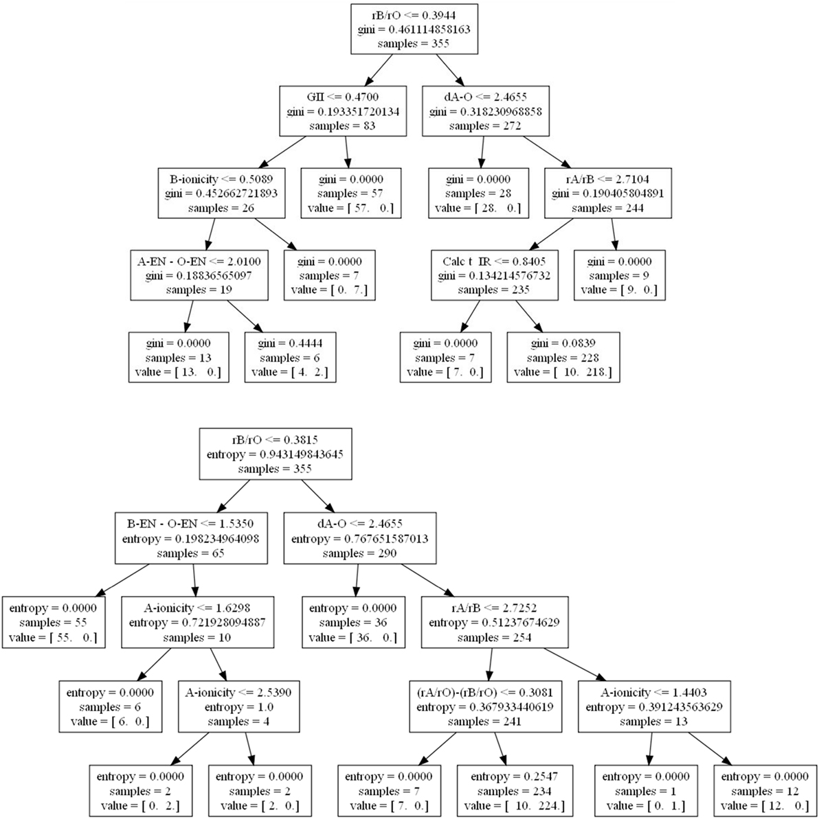
Figure 1. Decision trees for determining perovskite formability based on gini impurity (top) and Shannon entropy or information gain (bottom) using data from Balachandran et al. (2011). At each node, a check occurs and if true proceeds to the left and vice-versa. A value = (12, 0) would indicate given the prior conditions, 12 compounds do not form perovskites and 0 do.

Domain knowledge tells us that the tolerance factor, difference in ionic radii ratios, and A-site ionicity are proportional to the radius of the A-site cation, and are therefore expected to originate from close packing preferences of ionic solids. The GII is dependent on the difference between ideal and calculated bond valences, which can capture local bonding effects in addition to the steric packing preferences. Importantly, if the GII has useful predictive power for the cubic perovskite oxide stability relative to the binary oxide phases, which it may decompose into, more compounds could be screened than if only the radius based factors were predictive. Indeed, there are many cations with known bond valence parameters but lacking the necessary tabulated 12-coordinate ionic radii that may be used in the tolerance factor calculation. In addition, the incorporation of the GII in the model could elucidate additional bonding characteristics that lead to phase stability.

These trees were trained on the same data, so one would assume the same underlying physics should be captured by both, but that is not entirely the case. Building an optimally accurate tree is computationally expensive, and so heuristic algorithms are used instead, which are not guaranteed to find a global solution. Indeed, the resulting tree can vary even between multiple runs of the same algorithm. Increasing the number of allowed node layers might lead to convergence, but may also result in overfitting and/or a hard to explain tree. In this case, recreating the entropy-based model with a maximum depth of seven nodes yields a 95% accuracy confidence interval from 10-fold cross-validation of 93 (±12%) versus the original measure of 92 (±8%) with four nodes. The high level of accuracy in both cases indicates that a handful of structural features, such as ionic radii ratios and ideal A–O bond distance, are suitable to assess if an ABO₃ composition will the form the perovskite structure.

As an interesting aside, switching the number of partitions from 10 to 5 reduces the accuracy to ~90% for both node amounts. That is, changing the proportion of data used for training from 90 to 80% causes a non-trivial reduction in accuracy on average. Such a variation in performance from changing how the data is split indicates a sensitivity of the model to new data, and we would expect this model to not perform as well at predicting new compounds’ formability as cross-validation had led us to believe. In general, one should not assume default hyperparameters such as the number of folds are always optimal nor that cross-validation alone can give a “ground state” truth. Cross-validation is an optimistic guess that only works if the data supplied appropriately samples the underlying population. We are not saying here that one tree is definitely wrong and one is definitely right, but rather that any given model found in the literature is the result of numerous choices on behalf of the modeler. Domain knowledge should be applied to evaluate a model’s success in combination with the reported error bounds.

Descriptor Selection

Materials informatics trades in physically meaningful parameters. So-called descriptors of materials properties are key to making predictions and building understanding of systems of interest (Rondinelli et al., 2015). Some properties of a good descriptor have been laid out previously (Ghiringhelli et al., 2015). Namely, a good descriptor should be simpler to determine than the property itself, whether it is computationally obtained or experimentally measured. It should also be as low-dimensional as possible, and uniquely characterize a material. Descriptors in materials science can come from a variety of levels of complexity. Atomic numbers, elemental groups or periods, electronegativities, and atomic radii can be read off periodic tables and used to predict structure type. A compound’s free energy can be calculated using density functional theory and related to phase stability. Densities and structural parameters can be measured in an experiment for the purposes of predicting mechanical properties. And of course, combinations of quantities from the same or different levels can be descriptors as well.

There is, however, no universally acknowledged method for choosing descriptors. Descriptor choice will depend heavily upon the phenomena being studied. For instance, atomic radii happen to be important in predicting bulk metallic glass formation (Inoue and Takeuchi, 2004) as well as perovskite formability (Balachandran et al., 2011). However, attempting to use covalent radii for both will miss the important ionic character of the atoms in perovskite systems. Furthermore, one can benefit from analyzing data and research that is not directly related to one’s own for missing connections. Brgoch et al. had to confront the problem of complications in describing the excited state properties of inorganic phosphors with ab initio methods (Brgoch et al., 2013). An insight came from reading the literature on molecular phosphors, where structural rigidness played a key role in photoemission yield. With this knowledge, the authors were able to construct a descriptor for photoluminescent quantum yield in solids based on the Debye temperature, related to the stiffness of the vibrational modes, and band gap. A similar recognition of the underlying physics yielded a descriptor for carrier mobility in thermoelectrics based on bulk modulus and band effective mass (Yan et al., 2015). One review (Curtarolo et al., 2013) lays out several material descriptors that have been previously developed and proposes possibly overcoming the stipulation of having a physically meaningful descriptor by use of machine learning. However, it remains a challenge to motivate further exploration without an underlying theoretical justification.

Feature Extraction

In some cases, the best model may not be capable of being built from the features initially selected. A simple example might be predicting an activation energy from observed diffusion measurements using regression analysis. Using the natural log of diffusion constants yields a better fit than fitting the raw values.

Depending upon the material system of interest one can enumerate as many physically plausible primary descriptors as possible and then generate new descriptors from them in some manner. This could include groupings from dimensional analysis (Rajan et al., 2009), simple relational features (Kanter and Veeramachaneni, 2015), PCA (Sieg et al., 2006), or some other method. In all cases, care must be taken to avoid incompatible operations (e.g., do not add an atomic radius to an ionization potential). In image data, edges are often extracted as features from primary pixel data to be used in learning (Umbaugh, 2010). Commercial software such as Eureqa can be used to quickly generate function sets such as Gaussian and exponential functions among others (Dubčáková, 2010). Once features have been extracted, there might then be some downselection to test only the most important features. Ghiringhelli et al. (2015) successfully used feature extraction in combination with LASSO-based compressive sensing (Nelson et al., 2013) to generate descriptors for the energy difference between zinc blende or wurtzite and rock salt structure for 68 octet binary compounds.

Model Interpretability

Materials scientists are interested in establishing clear causal relations between materials structure defined broadly across length scales and properties. While a model employed by Netflix might be evaluated solely in terms of predictive accuracy and speed, scientific models have further constraints such as a minimal number of parameters and adherence to physical laws. If a model cannot be communicated clearly except from computer to computer, its contribution will be minimal. It is the obligation of the modeler to translate the results of their work into knowledge other materials scientists can use in aiding materials discovery or deployment. That being said, eliminating parameters by hand to make an intelligible model is often impractical. In this case, there are some helpful techniques available.

Principal Component Analysis

Principal component analysis is a powerful technique for data dimensionality reduction. In essence, PCA is a change of basis for your data with the new axes [principal components (PCs)] being linear combinations of original variables. Each principal component is chosen so that it lies along the direction of largest variance while being uncorrelated to other PCs. When the data are standardized to have zero mean, these PCs are eigenvectors to the covariance matrix of the samples. Although perfect description of the original data requires as many PCs as original features in theory, typically, some number of PCs is selected for retention based upon a threshold amount of variance explained or correlation with a feature of interest. In this manner, an effective description of a dataset with thousands of variables can be constructed from a few hundred PCs (Ringnér, 2008).

However, care must be taken to judiciously apply PCA. Authors will readily acknowledge PCs are not necessarily simple to interpret physically especially with image data (Belianinov et al., 2015a). PCA is not guaranteed to separate clusters of data from one another (Ringnér, 2008), and overzealous projection onto PCs can actually make classes of data inseparable that were previously separable before PCA (Figure 2).

FIGURE 2

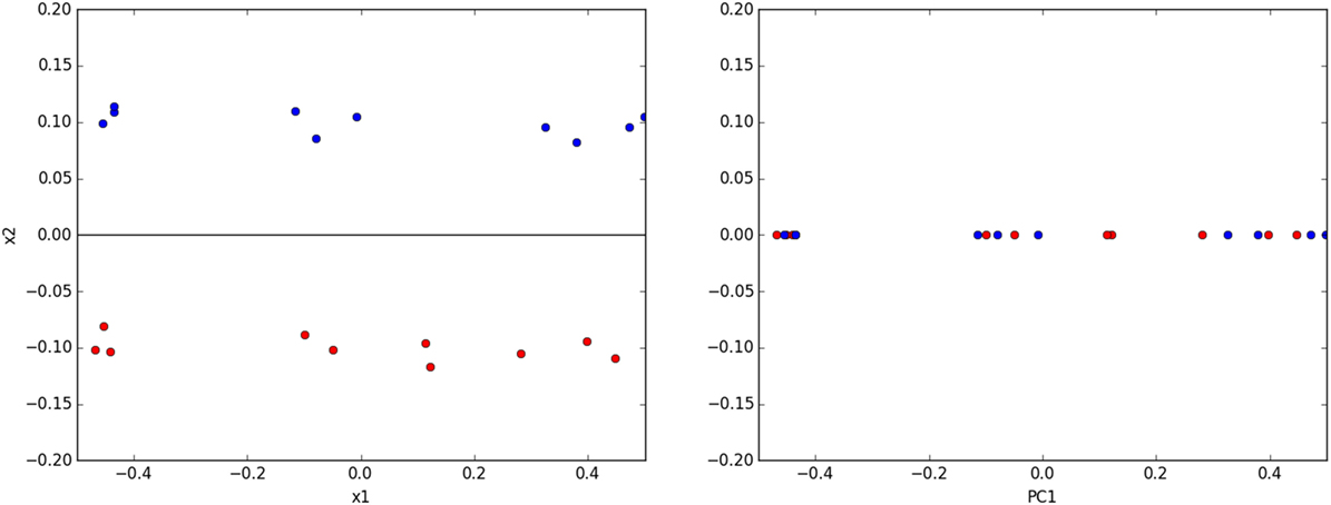
Figure 2. (left) A toy classification dataset consisting of two linearly separable classes. The ideal subspace produced with PCA is shown in black. (right) Projecting data onto this subspace destroys the original separability of the data.

In the example of rare earth vanadate oxide perovskites (RVO₃, R = Y, Yb, Ho, Dy, Gd, Pr, Nd, Ce, La), the orthorhombic Pnma structures of the family can be quantified using symmetry-adapted distortion modes (Perez-Mato and Aroyo, 2010). First, each mode represents a different collective atomic displacement pattern from the ideal cubic phase that appears in the Pnma structure; for example, in-phase VO₆ octahedral rotations (${\text{M}}_3^{+}$), out-of-phase octahedral rotations, (${\text{R}}_4^{+}$), antipolar R-cation displacements (${\text{X}}_5^{+}$ and ${\text{R}}_5^{+}$), or first-order Jahn-Teller distortions of the VO₆ octahedra (${\text{M}}_2^{+}$). Next, the net atomic displacements involved in each mode, which are required to reach the observed structure, are obtained as a root-sum-squared displacement magnitude in angstroms through this structural decomposition. These mode amplitudes can then be checked for correlations among each other and macroscopic observables, including the magnetic spin (T_N) and orbital ordering (T_OO) temperatures to identify whether a link between the atomic structure and magnetic and electronic transitions exists.

Figure 3 shows the Pearson correlation coefficients for each pair of features in the room-temperature vanadate dataset. The dark red squares indicate large positive correlation, while dark blue indicates large negative correlation. Greenish hues indicate little or no correlation. All modes which alter the shape and connectivity of the VO₆ octahedra are highly positively correlated with each other, but they are also strongly correlated and anti-correlated with T_OO and T_N, respectively.

FIGURE 3

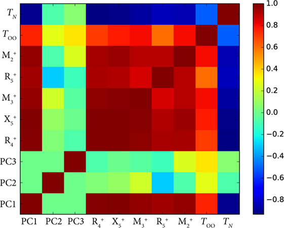
Figure 3. Plot of the Pearson correlation coefficients for the symmetry-adapted distortion mode (Balachandran et al., 2016) amplitudes and their first three principal components with orbital ordering temperature (T_OO), and Néel temperature (T_N) of the RVO₃ (R = rare earth) orthorhombic series of perovskites. PCA works well here because all the distortions correlate strongly with R cation size due to packing arguments.

This correlation among the modes can be reduced by performing a PCA (Table 1). Because changing the R cation alters each of the mode amplitudes by approximately the same proportion, much of the variance in the mode amplitudes can be explained by one PC: in Figure 3, we see the first PC, PC1, correlates strongly with every mode and the ordering temperatures. This analysis can allow us to disentangle the role of cation size in setting the ordering temperatures from other features in the structure. The reason this is possible is because the in-phase and out-of-phase rotations are both largely set by the cation size due to steric effects, which is gleaned from domain insight, and strongly coupled with the other modes such as the first-order Jahn-Teller distortions that directly affect orbital interactions through changes in V–O bond lengths (Varignon et al., 2015). Fundamentally, however, PCA explains variance in the data, and data can vary for reasons other than physically meaningful ones. The second PC (PC2) explains 3.2% of the variance and has large loadings from the ${\text{M}}_3^{+}$ and ${\text{R}}_5^{+}$ modes, but this could simply be due to noise in measurement or some other factor. A physical interpretation of this combination of in-phase VO₆ octahedral rotations and antipolar R-cation displacements causing the variation in T_OO or T_N requires further study. It also reinforces the view that although, PCA can potentially disentangle many factors, it requires careful interpretation.

TABLE 1

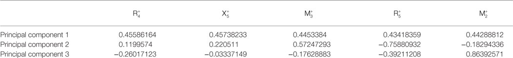
Table 1. Loadings of principal components.

When doing k-fold cross-validation, PCA must not be carried out on the entire dataset beforehand so as to avoid information contamination. Likewise, the weights for the PCs should not be modified for use on the testing set. If your dataset contains multiple variables that are correlated with one another, the PCs that best describe them will have an outsize level of variance explained. This means if the criterion for keeping a PC is based on a threshold variance explained, one might eliminate physically meaningful data from consideration in the model. For instance, in the PCA example shown in Figure 3, most of the variance in the distortion modes is due to changing cation size which alters octahedral rotation angles (${\text{M}}_3^{+}$ and ${\text{R}}_4^{+}$) and metal-oxygen bond lengths (${\text{M}}_2^{+}$). Keeping only the first PC might throw out features in the structure that could correlate subtly with ordering temperatures.

Cross-Validation and Regularization

Regularization of a model entails adding a tunable penalty on model parameter size to the cost function being minimized. Most frequently, regularization is used to reduce overfitting in linear regressions where it is commonly known by the names LASSO (minimizes the sum of absolute values of the fit parameters) and ridge regression (minimizes the sum of squares of the parameters). Unfortunately, no efficient computation is known for minimizing the number of non-zero coefficients directly, but these approximations often work well. The regularization penalty weight is increased (in powers of ten usually) iteratively and scored with cross-validation until a minimal test error is reached. As the penalty increases more and more model coefficients are driven to 0. The longer a coefficient remains non-zero, the more important it is to the model’s performance.

One caveat is that methods such as LASSO and ridge regression will drop correlated features more or less at random. If A predicts feature B and target C, one’s model may show B predicting C because regularization viewed A as redundant information. For instance, a bond energy may be correlated with melting point and elastic modulus, but LASSO may toss out the bond energy in favor of melting point when trying to predict the modulus even though direct causality is absent. One can brute force check for covariance between features, but this may be infeasible with large feature sizes or parameters in the descriptor. Thus, authors have adapted cross-validation methods that not only take random sets of samples but random features as well (Ghiringhelli et al., 2015). Ensemble methods such as random forests work in much the same manner by combining numerous different simple estimators like decision trees and averaging their parameters (Halawani, 2014). Hyperparameters such as the regularization penalty weight, number of simple learners in an ensemble, fraction of features/samples to randomly use, etc. should be iterated over in a cross-validation workflow to test that the final predictor is as simple as possible but no simpler.

Choice of Model

Related to above, the choice of machine learning model may have a large impact on how easy it is to comprehend for humans. Regressions and their regularized counterparts have coefficients whose size tells one the relative effect size of modifying an input on the output. Decision trees have a structure much like a flowchart that is easy to follow. Bayesian methods allow one to explicitly encode prior knowledge (Robert, 2001; Davidson-Pilon, 2015). On the other hand, some models such as kernelized support-vector machines and kernel ridge regression involve non-linear transformations that lead to obfuscation of the relationship between the original features and the target variable. Neural networks are another instance where a clear explanation of the machine’s “thinking” is usually impossible due to complex node interactions.

When given a choice, it may sometimes be worth a small tradeoff in cross-validation predicted accuracy for better explanatory power when comparing two candidate models. For example, in the perovskite formability case above, using a more complicated gradient boosted decision tree reduced the variance in the cross validation accuracy a few percentage points, but did not allow for a simple visual schematic (Pilania et al., 2015). Data transformations that lead to further abstraction like PCA should not be used as inputs to models if there is no clear reason why features should be covariant. A model with clear justification for why it possesses the uncertainty it has is less likely to result in unpleasant surprises later.

A Sample Workflow

Because there is no universally agreed upon workflow for a materials informatics problem, we make an attempt at describing one possibility as others have done (Ghiringhelli et al., 2015; Lookman et al., 2016). Our workflow can be divided into four sections as depicted in Figure 4.

FIGURE 4

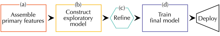
Figure 4. A schematic of the steps involved in designing a materials informatics model. The workflow starts with (A) collection of data relevant to the property of interest. Next, comes (B) building a simple model to explore correlations followed by (C) refinement of the model to satisfactory predictive accuracy and (D) final training and deployment. Starting with a less complex model supports a priori physical reasoning instead of post facto explanations.

Like any materials science problem, one should begin with accessing what domain knowledge already exists (Figure 4A). This domain knowledge should then be used to enumerate a first set of features that will be collected and processed for use in a model. Picking the right primary features is often the biggest determinant of the final predictor’s performance. The role of the machine learning algorithms is to find underlying structure in the data, not to make correlation where none exists. The selection of primary features overlaps in many ways with that of descriptors as explained earlier.

Once the primary features have been assembled and made ready for parsing, it is common practice to make an exploratory model with something like ridge regression or a decision tree and vary the features to begin understanding which of them are the most important in the model formulation (Figure 4B). Observe the effect of adding or removing primary features on the cross-validation measured error and contextualize this within your prior expertise. It is not recommended to jump straight into using the most complicated model, e.g., neural networks or kernel ridge regression, available as this will take much more time from both the researcher and the computer than eliminating spurious factors early on with domain knowledge. Sometimes a simple model following Occam’s razor is all that will be needed to reach the desired level of accuracy and explanatory power.

If none of the primary features show much more of a correlation with the output than would be expected from chance, this is an indication that either the sampling is bad or the causal feature is missing from the data. As a rule of thumb, if the number of samples is 10 times the number of features and no significant correlation is seen, there is likely something being missed.

If the model’s performance is significantly better than chance but could be better, this indicates there is an underlying pattern to the data but something needs refinement (Figure 4C). If there are few samples of a certain type, one may need to collect more or use one of the other methods for underrepresented data (García et al., 2007). Eliminating features with low impact on accuracy from early testing may reduce the level of noise a model has to contend with.

If the features are highly correlated with each other, a data dimension reduction technique like PC analysis, as discussed above, can eliminate redundant information. If one has reason to suspect some functional transformation of the data could help (e.g., for properties determined from constitutive relationships), feature extraction techniques can be used and the results trimmed down by intuition or algorithmically using a technique like LASSO (Ghiringhelli et al., 2015) or feature ranking from an ensemble method like boosted gradient decision trees (Pilania et al., 2015).

Last but not least, the type of machine learning algorithm chosen can impact the performance as well. A good workflow will have several types of models that are compared using cross-validation rather than picking just one initially. Each algorithm has its strengths and weaknesses. Random forests are known to be accurate and resistant to outliers but slow to train for large datasets. Naive Bayesian classifiers are very fast to train but produce unreliable probability estimates. Knowledge of the relative pros and cons for a given algorithm is strongly recommended before use [see for example Ref. Scikit-learn developers (2014) and Raschka (2015)].

Once refinement yields a satisfactory choice of model and hyperparameters, the last step before deployment is to train on the whole dataset to maximize the information contained in the final model (Figure 4D). The final round of cross-validation performed before this should provide a reasonable margin of error in line with your prior domain knowledge.

By proceeding in an iterative fashion upwards in complexity, one can avoid much of the backtracking to find a simpler model that would be required if proceeding less deterministically. Once the model performance is acceptable, its important findings should be broken down into guidelines and new data generated to improve the description further.

Conclusion

We have shown some of the things to be aware of when applying machine learning techniques to materials science. There is much more that could be discussed, and with such rapid innovations in machine learning, some of the techniques presented here are bound to become obsolete. What will not change is the importance of scientific reasoning in discovering reliable structure–property-processing models. The role of theorists and experimentalists in identifying descriptors and quantifying uncertainty has never been more important. Data without science are like marble without a sculptor, trapped beauty waiting to be set free.

Author Contributions

JR supervised the research and NW performed the simulations and analysis. NW wrote the first draft of the manuscript and both authors edited and commented on the manuscript.

Conflict of Interest Statement

The authors declare that the research was conducted in the absence of any commercial or financial relationships that could be construed as a potential conflict of interest.

Acknowledgments

NW and JR thank L. Ward, P.V. Balachandran, and colleagues at the 2015 Opportunities in Materials Informatics Conference for useful discussions.

Funding

NW and JR were supported from DOE grant number DE-SC0012375 for the machine learning analysis and NSF DMR-1454688, respectively.

References

Balachandran, P., Broderick, S., and Rajan, K. (2011). Identifying the ‘inorganic gene’ for high-temperature piezoelectric perovskites through statistical learning. Proc. R. Soc. A 467, 2271–2290. doi:10.1098/rspa.2010.0543

CrossRef Full Text | Google Scholar

Balachandran, P. V., Benedek, N. A., and Rondinelli, J. M. (2016). “Symmetry-adapted distortion modes as descriptors for materials informatics,” in Information Science for Materials Discovery and Design, Vol. 225, eds T. Lookman, F. J. Alexander, and K. Rajan (Switzerland: Springer International Publishing), 213–222.

Google Scholar

Belianinov, A., He, Q., Kravchenko, M., Jesse, S., Borisevich, A., and Kalinin, S. (2015a). Identification of phases, symmetries and defects through local crystallography. Nat. Commun. 6, 7801. doi:10.1038/ncomms8801

PubMed Abstract | CrossRef Full Text | Google Scholar

Belianinov, A., Vasudevan, R., Strelcov, E., Steed, C., Yang, S. M., Tselev, A., et al. (2015b). Big data and deep data in scanning and electron microscopies: deriving functionality from multidimensional data sets. Adv. Struct. Chem. Imaging 1, 1–25. doi:10.1186/s40679-015-0006-6

CrossRef Full Text | Google Scholar

Botu, V., Mhadeshwar, A. B., Suib, S. L., and Ramprasad, R. (2016). “Optimal dopant selection for water splitting with cerium oxides: mining and screening first principles data,” in Information Science for Materials Discovery and Design, Vol. 225, eds T. Lookman, F. J. Alexander, and K. Rajan (Switzerland: Springer International Publishing), 157–171.

Google Scholar

Brgoch, J., DenBaars, S., and Seshadri, R. (2013). Proxies from Ab initio calculations for screening efficient Ce³⁺ phosphor hosts. J. Phys. Chem. C 117, 17955–17959. doi:10.1021/jp405858e

CrossRef Full Text | Google Scholar

Cawley, G., and Talbot, N. (2010). On Over-fitting in Model Selection and Subsequent Selection Bias in Performance Evaluation. J. Mach. Learn. Res. 11, 2079–2107.

Google Scholar

Curtarolo, S., Hart, G., Nardelli, M., Mingo, N., Sanvito, S., and Levy, O. (2013). The high-throughput highway to computational materials design. Nat. Mater. 12, 191–201. doi:10.1038/NMAT3568

PubMed Abstract | CrossRef Full Text | Google Scholar

Dalton, L. A., and Dougherty, E. R. (2016). “Small-sample classification,” in Information Science for Materials Discovery and Design, Vol. 225, eds T. Lookman, F. J. Alexander, and K. Rajan (Switzerland: Springer International Publishing), 77–101.

Google Scholar

Davidson-Pilon, C. (2015). Bayesian Methods for Hackers. New York: Addison-Wesley Professional.

Google Scholar

Dubčáková, R. (2010). “Eureqa – software review,” in Genetic Programming and Evolvable Machines, Vol. 112 (Netherlands: Springer US), 173–178.

Google Scholar

Featherston, C., and O’Sullivan, E. (2014). A Review of International Public Sector Strategies and Roadmaps: A Case Study in Advanced Materials. Cambridge: Centre for Science Technology and Innovation, Institute for Manufacturing, University of Cambridge.

Google Scholar

García, V., Sánchez, J., Mollineda, R., Alejo, R., and Sotoca, J. (2007). “The class imbalance problem in pattern classification and learning,” in II Congreso Español de Informática. Zaragoza.

Google Scholar

Ghiringhelli, L., Vybiral, J., Levchenko, S., Draxl, C., and Scheffler, M. (2015). Big data of materials science: critical role of the descriptor. Phys. Rev. Lett. 114, 105503. doi:10.1103/PhysRevLett.114.105503

PubMed Abstract | CrossRef Full Text | Google Scholar

Halawani, S. M. (2014). A study of decision tree ensembles and feature selection for steel plates faults detection. Int. J. Tech. Res. Appl. 2, 127–131.

Google Scholar

Hautier, G., Fischer, C., Jain, A., Mueller, T., and Ceder, G. (2010). Finding nature’s missing ternary oxide compounds using machine learning and density functional theory. Chem. Mater. 22, 3762–3767. doi:10.1021/cm100795d

CrossRef Full Text | Google Scholar

Inoue, A., and Takeuchi, A. (2004). Recent progress in bulk glassy, nanoquasicrystalline and nanocrystalline alloys. Mater. Sci. Eng. A 375-377, 16–30. doi:10.1016/j.msea.2003.10.159

CrossRef Full Text | Google Scholar

Kamath, C. (2016). “On the use of data mining techniques to build high-density, additively-manufactured parts,” in Information Science for Materials Discovery and Design, Vol. 225, eds T. Lookman, F. J. Alexander, and K. Rajan (Switzerland: Springer International Publishing), 141–155.

Google Scholar

Kanter, J., and Veeramachaneni, K. (2015). “Deep feature synthesis: towards automating data science endeavors,” in IEEE International Conference on Data Science and Advanced Analytics. Cambridge, MA.

Google Scholar

Klanner, C., Farruseng, D., Baumes, L., Lengliz, M., Mirodatos, C., and Schüth, F. (2004). The development of descriptors for solids: teaching “catalytic intuition” to a computer. Angew. Chem. Int. Ed. 43, 5347–5349. doi:10.1002/anie.200460731

CrossRef Full Text | Google Scholar

Lookman, T., Alexander, F. J., and Rajan, K. (eds). (2016). “Preface,” in Information Science for Materials Discovery and Design, Vol. 225 (Switzerland: Springer International Publishing), v–vii.

Google Scholar

Lookman, T., Balachandran, P. V., Xue, D., Pilania, G., Shearman, T., Theiler, J., et al. (2016). “A perspective on materials informatics: state-of-the-art and challenges,” in Information Science for Materials Discovery and Design, Vol. 225, eds T. Lookman, F. J. Alexander, and K. Rajan (Switzerland: Springer International Publishing), 3–12.

Google Scholar

Lufaso, M. W., and Woodward, P. M. (2001). Prediction of the crystal structures of perovskites using the software program SPuDS. Acta Crystallogr. B 57, 725–738. doi:10.1107/S0108768101015282

PubMed Abstract | CrossRef Full Text | Google Scholar

National Science and Technology Council. (2011). Materials Genome Initiative for Global Competitiveness.

Google Scholar

Nelson, L., Hart, G., Zhou, F., and Ozoliņŝ, V. (2013). Compressive sensing as a paradigm for building physics models. Phys. Rev. B 87, 035125. doi:10.1103/PhysRevB.87.035125

CrossRef Full Text | Google Scholar

Perez-Mato, J. M., and Aroyo, M. I. (2010). Mode crystallography of distorted structures. Acta. Cryst. A66, 588–590. doi:10.1107/S0108767310016247

CrossRef Full Text | Google Scholar

Pilania, G., Balachandran, P., Gubernatis, J., and Lookman, T. (2015). Classification of ABO3 perovskite solids: a machine learning study. Acta. Crystallogr. B Struct. Sci. Cryst. Eng. Mater. 71, 507–513. doi:10.1107/S2052520615013979

PubMed Abstract | CrossRef Full Text | Google Scholar

Quinlan, J. (1986). Induction of decision trees. Mach. Learn. 1, 81–106. doi:10.1023/A:1022643204877

CrossRef Full Text | Google Scholar

Rajan, K. (2005). Materials informatics. Mater. Today 8, 38–45. doi:10.1016/S1369-021(05)71123-8

CrossRef Full Text | Google Scholar

Rajan, K., Suh, C., and Mendez, P. (2009). Principal component analysis and dimensional analysis as materials informatics tools to reduce dimensionality in materials science and engineering. Stat. Anal. Data Min. 1, 361–371. doi:10.1002/sam

CrossRef Full Text | Google Scholar

Raschka, S. (2015). Python Machine Learning. Birmingham: Packt Publishing.

Google Scholar

Ringnér, M. (2008). What is principal component analysis? Nat. Biotechnol. 26, 303–304. doi:10.1038/nbt0308-303

CrossRef Full Text | Google Scholar

Robert, C. (2001). The Bayesian Choice: From Decision-Theoretic Foundations to Computational Implementation (Springer Texts in Statistics). New York: Springer-Verlag.

Google Scholar

Rokach, L., and Maimon, O. (2005). Top-down induction of decision trees classifiers-a survey. IEEE Trans. Syst. Man Cybern. C Appl. Rev. 35, 476–487. doi:10.1109/TSMCC.2004.843247

CrossRef Full Text | Google Scholar

Rondinelli, J. M., Poppelmeier, K. R., and Zunger, A. (2015). Research update: towards designed functionalities in oxide-based electronic materials. Appl. Phys. Lett. Mater. 3, 080702. doi:10.1063/1.4928289

CrossRef Full Text | Google Scholar

Scikit-learn developers. (2014). Scikit Learn website. Available at: http://scikit-learn.org/stable/user_guide.html

Google Scholar

Sieg, S., Suh, C., Schmidt, T., Stukowski, M., Rajan, K., and Maier, W. (2006). Principal component analysis of catalytic functions in the composition space of heterogeneous catalysts. QSAR Comb. Sci. 26, 528–535. doi:10.1002/qsar.200620074

CrossRef Full Text | Google Scholar

Stone, M. (1974). Cross-validatory choice and assessment of statistical predictions. J. R. Stat. Soc. Series B (Methodol.) 36, 111–147.

Google Scholar

Umbaugh, S. (2010). Digital Image Processing and Analysis: Human and Computer Vision Applications with CVIPtools, 2nd Edn. Boca Raton, FL: CRC Press.

Google Scholar

Varignon, J., Bristowe, N. C., Bousquet, E., and Ghosez, P. (2015). Coupling and electronic control of structural, orbital and magnetic orders in perovskites. Sci. Rep. 5, 15364. doi:10.1038/srep15364

CrossRef Full Text | Google Scholar

Yan, J., Gorai, P., Ortiz, B., Miller, S., Barnett, S., Mason, T., et al. (2015). Material descriptors for predicting thermoelectric performance. Energy Environ. Sci. 8, 983–994. doi:10.1039/c4ee03157a

CrossRef Full Text | Google Scholar