A Phase Space Approach to Supercooled Liquids and a Universal Collapse of Their Viscosity

1. Introduction

Human kind has been forming and using glasses for millennia. The unique optical, thermal, and mechanical properties, as well as ease of working, which arises from the lack of long-range crystalline order in glasses (Gupta, 1996) has lead to their application in a diverse range of fields (Zallen, 1983; Hancock and Parks, 2000; Telford, 2004; Greer and Ma, 2007; Wuttig and Yamada, 2007; Berthier and Ediger, 2016). Despite their ubiquity, a fundamental understanding of the phenomenology associated with glasses and their formation via the vitreous transition remains elusive. In order to understand the structural and mechanical behavior of glasses, we must first understand how and why they form at all. As glasses form from supercooled liquids, this means we must first understand the dynamics of supercooled liquids. Ordinarily, when an equilibrium liquid is cooled to a temperature beneath its melting point it undergoes a first order thermodynamic transition to the ordered crystalline solid. However, if the liquid is cooled sufficiently quickly (at material-dependent rate), crystallization can be bypassed, and the liquid enters a metastable (with respect to the crystal) state and is termed “supercooled.” The thermodynamic and kinetic properties of supercooled liquids exhibit a number of remarkable characteristics, but the most striking is arguably the behavior of the viscosity (and all associated relaxation times) (Cavagna, 2009; Procaccia, 2009; Berthier and Biroli, 2011; Hunter and Weeks, 2011; Kalogeras and Hagg Lobland, 2012; Langer, 2014). The viscosity of supercooled liquids grows by as much as 14 decades over temperature ranges as small as a few hundred Kelvin, eventually reaching a value of 10¹² Pa s at the kinetic glass “transition” that occurs at a temperature T_g. Calorimetric signatures of the transition into the glassy state have also been observed at the dynamic glass transition temperature T_g (Yue, 2009). At temperatures below the glass transition temperature, T_g, the increasingly sluggish dynamics lead to the onset of rigidity and solid-like behavior in the liquid on observable timescales. This immense dynamical slowing occurs without any obvious structural change/ordering and attempts to find an appropriate order parameter or growing length scale have remained inconclusive. As such, explaining the spectacular increase of the viscosity (and associated relaxation time) of supercooled liquids remains an open challenge in material science.

Liquids, which are in equilibrium at high temperatures above melting, have a viscosity that is well described by an Arrhenius function, namely,

$\eta \left(T\right)={\eta }_0{e}^{\frac{\mathrm{\Delta }G\left(T\right)}{k_{B}T}},$ (1)

with ΔG(T), a (weakly) temperature-dependent Gibb’s free energy of activation and k_B, Boltzmann’s constant. The simple interpretation of this form is that there exists a well-defined energy barrier (associated with bond-breaking) that can be overcome by thermal excitations. As the temperature is lowered, appropriately sized thermal fluctuations become considerably less likely and flow decreases appreciably. If this form were maintained in the supercooled liquid, there would be little mystery. However, all liquids show a degree of departure from the Arrhenius form. This degree of departure forms a continuous spectrum and is quantified by Angell’s fragility parameter (Angell, 1995; Angell et al., 2000). According to this scheme, the most “fragile” liquids (those with the high values of the fragility parameter) display a far more dramatic rise in the viscosity than that predicted by an Arrhenius law, whereas the deviation from an Arrhenius law is far smaller in “strong” liquids (having a small fragility). The underlying physics of the departure from equation (1) is what we aim to explain.

Some of the first attempts to describe the non-Arrhenius character of supercooled liquid viscosity were undertaken in the 1920s by Vogel (1921), Fulcher (1925), and Tammann and Hesse (1926). Collectively, they discovered that the functional form,

$\eta \left(T\right)={\eta }_0{e}^{\frac{D{T}_0}{T-T_0}}$ (2)

was able to adequately describe the viscosity of many supercooled liquids over a fair range of temperatures. In the so-called VFTH form, the parameter D is related to the fragility, and T₀ is a material-dependent temperature at which a dynamic divergence is predicted to occur. This form initially appeared as a purely empirical form, with no rigorous theoretical support. However, over the years a number of theoretical frameworks have been proposed (Cohen and Turnbull, 1959; Adam and Gibbs, 1965; Bengtzelius et al., 1984; Leutheusser, 1984; Kirkpatrick et al., 1989; Parisi and Mezard, 1999; Lubchenko and Wolynes, 2007; Gotze, 2008) to reproduce the VFTH form. While the VFTH form has survived for nearly a century and is widely used, it has consistently been shown to provide an overall poor fit to the viscosity of supercooled liquids of all types (classes, fragilities, bonding types, etc.) over the whole range of data. Additionally, there is no conclusive evidence for a dynamic divergence at any temperature above absolute zero (Mauro, 2011). These include tantalizing experiments that employed 20-million-year-old amber (Mauro, 2011; Zhao et al., 2013). For these and other reasons, a plethora of other functional forms have been proposed in the last 30 years, which do not contain a dynamic divergence and which have rigorous theoretical foundations. A few of these, which have been found to accurately describe the viscosity of many glass-forming liquids, are the KKZNT, Cohen–Grest free volume, parabolic, and MYEGA forms (Cohen and Grest, 1979; Kivelson et al., 1995; Nussinov, 2004; Tarjus et al., 2005; Elmatad et al., 2009, 2010; Mauro et al., 2009).

The aforementioned functional forms have all been shown to do an excellent job of reproducing the temperature dependence of the viscosity of a wide range of supercooled liquids. For example, the KKZNT form (Kivelson et al., 1995; Nussinov, 2004; Tarjus et al., 2005) has become a favorite of some researchers in the metallic glass community and very accurately describes the behavior of metallic liquids (Blodgett et al., 2015), while the MYEGA form (Mauro et al., 2009) has become ubiquitous in the silicate and oxide glass community, as it works very well for covalently bonded non-organic liquids. The trouble with these forms, as we will show, is that despite their applicability to some liquids they do not accurately describe all types of supercooled liquids. This is made particularly striking in a review by Angell et al. (2000), in which the authors list ten different functional forms all of which they discuss are accurate only for certain types/classes of liquids. Additionally bothersome is that most of these theories contain at least three adjustable parameters, which cannot be uniquely determined by correlations with thermodynamic observables. This is true of the parabolic form (Elmatad et al., 2009, 2010), which has wide applicability to fragile glasses. It seems reasonable to expect that if any liquid can in principle be supercooled, then there should be some universal mechanism/theory that is applicable across all liquids. Further, the material-dependent parameters of a given model should be related to thermodynamic observables, and not arbitrary fitting variables, while reflecting first principles.

In order to remedy the issues discussed above, we will now propose and assess a classical statistical mechanical framework to describe the viscosity of supercooled liquids. An earlier quantum rendition of our theory that mirrors and contains many of the considerations invoked in the classical approach that we discuss here first appeared in Nussinov (2015) and motivated the fit and collapse that we experimentally tested and derive here classically. Within our framework, the temperature dependence of the viscosity contains only a single parameter. Such a functional dependence implies a collapse of the viscosity data. In the current work, we collapse the published viscosity data of 45 supercooled liquids onto a single scaling curve. This collapse is a central result of our work. Additional aspects of our approach (in particular, the calculation of Angell’s fragility parameter and the viscosity above the melting temperature) along with further details concerning our data analysis and fits appear in Weingartner et al. (2015). Regardless of our theoretical bias, the existence of the universal collapse of the viscosity data that we first report on here suggests [as it has in many other arenas for very different problems (Stanley, 1999; West and Brown, 2005; Pyrak-Nolte and Nolte, 2016)] an underlying simplicity. Historically, the existence of a collapse in which the data from numerous systems were seen to fall on a universal curve pointed to a commonality in standard equilibrium critical phenomena (Stanley, 1999). Historically, the discovery that experimental data for various systems in the vicinity of their liquid to gas phase transition can be made to collapse onto a single curve after a simple rescaling (Guggenheim, 1945) predated current understanding of critical phenomena by many decades and hinted at the universality that permeates equilibrium phase transitions (Stanley, 1999; Nishimori and Ortiz, 2010). We hope that the viscosity collapse that we find for all studied supercooled liquids will spur further investigation. In the next section, we turn to the rudiments of our classical statistical mechanics approach.

2. Fundamentals of the Energy Shell Distribution Approach

The macroscopic thermodynamic and dynamical observables (such as viscosity) of a many-body system ultimately result from the average of the microscopic dynamics of the constituent atoms of the system. These microscopic dynamics are governed by the interactions between the system’s constituent members, and these are encoded in the system’s Hamiltonian, H, which is a function of the kinetic and interaction energies of the constituent atoms in the system. We can write down the exact classical, many-body Hamiltonian for a supercooled liquid of any type as

$\begin{array}{ll}H={\displaystyle \sum _i}\frac{{\overrightarrow{P}}_i^2}{2M_i}+{\displaystyle \sum _i}\frac{{\overrightarrow{p}}_i^2}{2m_e}+{\displaystyle \sum _{i>i^{\prime }}}\frac{e^2}{4\pi {\mathrm{ϵ}}_0|{\overrightarrow{r}}_i-{\overrightarrow{r}}_{i^{\prime }}|}\hfill & \hfill \\ +{\displaystyle \sum _{\mathit{ij}}}\frac{Z_i{e}^2}{4\pi {\mathrm{ϵ}}_0|{\overrightarrow{R}}_j-{\overrightarrow{r}}_i|}+{\displaystyle \sum _{j>j^{\prime }}}\frac{Z_i{Z}_j{e}^2}{4\pi {\mathrm{ϵ}}_0|{\overrightarrow{R}}_j-{\overrightarrow{R}}_{j^{\prime }}|}.\end{array}$ (3)

where Z_i is the atomic number, m_e is the electron mass, M_i is the atomic mass, ${\overrightarrow{r}}_i$ is the position of the i-th electron, and ${\overrightarrow{R}}_j$ is the position of the j-th nucleus. We consider realistic three-dimensional liquids of N particles (the total number of electrons and nuclei). This Hamiltonian is intentionally general; changing the values of Z_i, M_i, and the specific form of any additional interaction potentials allows one to describe any and all specific liquids. Although the exact Hamiltonian is given by equation (3), this precise form of the Hamiltonian will be immaterial in the very general analysis that follows. Rather, as we will explain, what matters most in our classical approach [and in its quantum analog (Nussinov, 2015)] is that the equilibrium properties of this disorder-free many-body Hamiltonian are empirically well known. Specifically, the realization of Hamiltonian of equation (3), as it pertains to standard disorder free materials, typically exhibits equilibrium solid or liquid phase at, respectively, low or high energy densities or temperatures.

In what briefly follows, we denote the collection of the momentum coordinates of all particles (electrons and nuclei) by $\overrightarrow{\pi }$ and the collection of all spatial coordinates by $\overrightarrow{x}$. To compute the dynamics of constituents of the liquid, one needs to solve Hamilton’s equations,

$\begin{array}{llll}\hfill \dot{\overrightarrow{\pi }}& =-{\nabla }_{\overrightarrow{x}}H& \hfill & \\ \hfill \dot{\overrightarrow{x}}& ={\nabla }_{\overrightarrow{\pi }}H\end{array}$ (4)

given the Hamiltonian in equation (3). In general, for a many-body system such as a liquid, this leads to a set of strongly coupled, highly non-linear, partial differential equations, which are impossible to solve exactly. For our purposes, however, it will suffice to rely only on simple statistical mechanics ideas in conjunction with extensively verified experimental observations.

The state of a classical N-body system may be represented by a point labeled by the positions and momenta of each of the particles in 6N-dimensional phase space [a microstate $\left(\overrightarrow{x},\overrightarrow{\pi }\right)$]. The time evolution of the system defines a trajectory in this phase space. The system is assumed to be in any of the microstates, which are allowed by the external constraints of the system (macrostate), with appropriate statistical weights set by the specific ensemble being employed. The calculation of the average values of physical observables O proceeds by averaging the value of O of all microstates in the allowed region(s) of phase space. For an isolated system, the allowed phase space is given by a shell centered on the hypersurface of constant energy, $H\left(\overrightarrow{x},\overrightarrow{\pi }\right)=E$, with thickness δE set by the uncertainty in specification of the external energy. The statistical weights are constant in the allowed region and zero elsewhere, such that microcanonical averages are given by

$\overline{O}\left(E\right)=\frac{1}{D\left(E\right)}\int d^{3N}x\int \frac{d^{3N}\pi }{{\left(2\pi \hslash \right)}^{3N}}O\left(\overrightarrow{x},\overrightarrow{\pi }\right)\mathrm{\delta }\left(H\left(\overrightarrow{x},\overrightarrow{\pi }\right)-E\right),$ (5)

with the density of states

$D\left(E\right)=\int d^{3N}x\int \frac{d^{3N}\pi }{{\left(2\pi \hslash \right)}^{3N}}\mathrm{\delta }\left(H\left(\overrightarrow{x},\overrightarrow{\pi }\right)-E\right).$ (6)

When the system is coupled to an external heat bath, all energies are in principle attainable by the system, and the infinitesimally thick shell (δ-peaked) of allowed phase space (Figure 1) may become smeared and overlap. This leads to averages of the form

$\overline{O}=\int {\mathit{dE}}^{\prime }{\overline{O}}_m\left(E^{\prime }\right)\rho \left(E^{\prime }\right).$ (7)

FIGURE 1

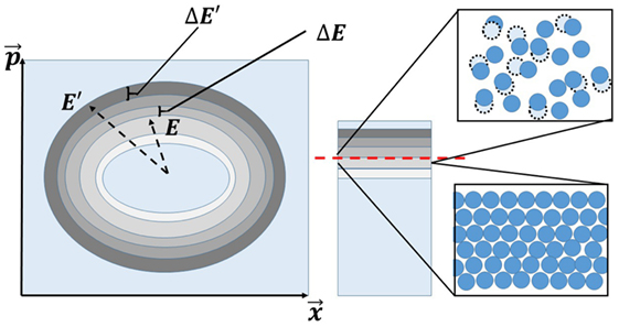
Figure 1. At left is a phase space schematic with fixed energy shells. As described in the text, the microstates change from being “liquid-like” at high energy densities (or associated high temperatures) to being “solid-like” at low energies (or low temperatures). On the right, we depict a cartoon of the atomic microstates both above and below the energy density associated with melting (dashed line at center).

Here, ${\overline{O}}_m\left(E^{\prime }\right)$ is the microcanonical average of O at an energy E′, and ρ(E′) is a (normalized) probability distribution in phase space, which is no longer a δ-function. In standard equilibrated systems [such as those corresponding to the disorder free Hamiltonian of equation (3) that describes equilibrated solids and liquids], the ensemble average of equation (7) is equal to the longtime average of O (which we denote by O_∞) as it evolves according to equations (4). Empirically, as we remarked earlier, at high enough temperatures or energy densities, the system of equation (3) is a fluid, while at temperatures or energy densities below that of freezing the system is an equilibrium solids. Thus, for any observable O, the microstate average of equation (5) will change character from featuring equilibrium fluid like features at high energies to solid-like behaviors at low energies. When latent heat appears at the equilibrium melting transition (as it nearly always does), there will be intermediate states displaying mixed fluid and solid like features (Nussinov, 2015). It follows that, when averaged over energy shells in phase space, the microstates themselves change their character across the equilibrium phase transitions. Figure 1 portrays the above simple conclusion.

Since systems in equilibrium, with a well-defined temperature, have a canonical partition function,

$Z={\int }_{-\infty }^{\infty }\mathit{dE}D\left(E\right)e^{-\frac{E}{k_{B}T}}.$ (8)

In this case, ρ(E′) corresponds to the Gibbs distribution, namely,

$\rho \left(E^{\prime }\right)=\frac{D\left(E^{\prime }\right)e^{-\frac{E^{\prime }}{k_{B}T}}}{Z}.$ (9)

If the system is cooled quasistatically, equilibrium will be maintained, and the distribution will remain canonical at progressively lower temperatures. This is, in part, guaranteed by Liouville’s theorem, which states that the phase space volume along trajectories in phase space is preserved for Hamiltonian systems. This means that as the system is cooled slowly enough, trajectories will neither bunch nor diverge and will map in a “1-to-1” fashion to the newly allowed region of phase space, and the distribution function will adjust accordingly. If instead of slow quasistatic cooling, we rapidly quench the system, it will cease to be in equilibrium and its dynamics will no longer be Hamiltonian. The now dissipative system will violate Liouville’s theorem: the trajectories from nearby points in phase space can diverge, and the phase space volume may swell. The initial shape of the initial energy shells will change due to supercooling. This shape deformation is central to our description of the supercooling process. Due to this non-adiabatic evolution, the Gibbs distribution will no longer be the exactly correct distribution describing the distribution in phase space. If we allow the system to maintain metastable equilibrium then the canonical ensemble is still roughly obeyed. However, in this case, different regions of the initial phase space will map to regions with, correspondingly, disparate effective canonical distribution functions, i.e., with different effective temperatures. This idea, which is seemingly reinforced by the appearance of dynamical heterogeneities (Kob et al., 1997; Donati et al., 1998; Sillescu, 1999; Ediger, 2000; Gebremichael et al., 2001; Richert, 2002; Nussinov, 2015) and other phenomena, implies that the overall system will sample a range of effective global temperatures (necessitated by the apparent spatial distribution of local effective temperatures) consistent with the externally imposed temperature, T. This distribution of effective temperatures forms the nub of our “Energy Shell Distribution Theory” (ESDT).

With the system now sampling a smeared out distribution of effective temperatures, the phase space probability distribution for the averages of equation (7) will now involve a conditional probability density ρ(E | T′) for the energy given a specific temperature, namely,

$\rho \left(E\right)=\int d{T}^{\prime }\rho \left(E|T^{\prime }\right)\rho \left(T^{\prime }\right).$ (10)

Here, ρ(T′) is the probability distribution of effective temperatures T′. As the system is in a metastable equilibrium, the probability density for a given E at a temperature T′ will still reasonably be described by the Gibbs distribution of equation (9). Similar to equation (7), the longtime average of O for a general distribution ρ including that associated with the supercooled liquid (sc) reads (Nussinov, 2015).

${\overline{O}}_{\infty ,\mathit{sc}}=\int d{T}^{\prime }\rho \left(T^{\prime }\right){\tilde{O}}_{\mathit{can}}\left(T^{\prime }\right).$ (11)

Here, ${\tilde{O}}_{\mathit{can}}\left(T^{\prime }\right)$ is the canonical, equilibrium value of the observable O at a temperature T′. We see, then, that supercooling acts to drive the system into a metastable equilibrium, which leads to the system sampling a range of equilibrium value averages over a narrow, but finite distribution of effective temperatures. The initial “shock” to the system of supercooling causes microscopic effects, which broaden the distribution. By virtue of being out of equilibrium, the distribution ρ must have a finite standard deviation (SD). This is so as otherwise the system would be described by a unique uniform effective temperature and be describable by the equilibrium canonical ensemble. However, since the supercooled liquid is out of equilibrium, the SD σ associated with the distribution ρ cannot vanish (Nussinov, 2015). When thermodynamic equilibrium is restored at a uniform global temperature T, the distribution ρ(T′) becomes a delta function (δ(T − T′)) implying an equilibrium Boltzmann distribution (and ensuing equilibrium expectation values for all observables).

With the above statistical mechanics ideas in place, we now invoke these to calculate the values of observables of interest. One method of measuring the viscosity of a liquid is by measuring the terminal velocity of a sphere dropped into the liquid. In this case, the viscosity is inversely proportional (η ∝ 1/v_∞) to the terminal velocity of the sphere. The terminal velocity is a macroscopic property of the system and therefore can be calculated in our statistical mechanical framework. Setting the observable O to be the vertical velocity of the dropped sphere, O = v_z (Nussinov, 2015), the observed terminal velocity becomes

${\overline{v}}_{\infty \text{,}\mathit{sc}}=\int d{T}^{\prime }\rho \left(T^{\prime }\right){\tilde{v}}_{\infty \text{,}\mathit{can}}\left(T^{\prime }\right).$ (12)

Thus, the viscosity will be given by

$\eta =\frac{A}{\int d{T}^{\prime }\rho \left(T^{\prime }\right){\tilde{v}}_{\infty ,\mathit{can}}\left(T^{\prime }\right)},$ (13)

with A as a constant. As is well known, for an equilibrium system, there exists a cutoff temperature, T_c, below which the terminal velocity must vanish (since the system is completely solid and no longtime flow occurs). Thus, in the equilibrium canonical ensemble, only averages of the terminal velocity at temperatures above this cutoff may contribute to the integral in equation (13) leading to

$\eta =\frac{A}{{\int }_{T_c}^{\infty }d{T}^{\prime }\rho \left(T^{\prime }\right){\tilde{v}}_{\infty ,\mathit{can}}\left(T^{\prime }\right)}.$ (14)

If we further assume that the distribution ρ is sufficiently narrowly peaked [as will be verified in the next section and seen from the numerical value of our fit parameter $\overline{A}$ (to be described therein)] such that the distribution has minimal “leakage” into effective temperatures T′ above T_c, when the measured global temperature T < T_c, then the value of v_∞,can will change very little over the region of appreciable weight. Therefore, we can reasonably replace v_∞,can(T′) with v_∞,can(T_c). Thus, the viscosity of the supercooled liquid is

$\eta =\frac{\eta \left(T_c\right)}{{\int }_{T_c}^{\infty }d{T}^{\prime }\rho \left(T^{\prime }\right)}.$ (15)

In order to use this expression to make concrete predictions of the viscosity, we must know what functional form to use for ρ(T′). All that is known about the distribution is that it is peaked about the external temperature, T, must be normalized, and that it has a small yet finite width. In the absence of additional constraints, the appropriate distribution ρ for the supercooled liquid may be ascertained (Nussinov, 2015) by maximizing the Shannon entropy $H_I=-\int \rho \left(T^{\prime }\right){\text{log}}_2\left[\rho \left(T^{\prime }\right)\right]d{T}^{\prime }$. As is well known, maximizing the Shannon entropy with the constraints of normalization and finite variance leads to a Gaussian distribution. Therefore, the most probable distribution of effective temperatures is

$\rho \left(T^{\prime }\right)=\frac{1}{\sqrt{2\pi }\tilde{O}\left(T^{\prime }\right)}{e}^{-\frac{{\left(T^{\prime }-T\right)}^2}{2\tilde{O}{\left(T^{\prime }\right)}^2}},$ (16)

where σ(T′) represents the spread of the distribution, and T is the external temperature. Inserting the Gaussian distribution of equation (16) into equation (15), we find that the viscosity

$\eta (T)=\frac{\eta (T_c)}{erfc\left[\frac{T_c-T}{\sqrt{2}\sigma (T)}\right]}.$ (17)

In what follows, we make two conjectures to complete the form of the viscosity, one involving the cutoff temperature and the other involving the spread of the Gaussian.

2.1. The Cutoff Temperature

In choosing a value for the cutoff temperature, T_c, we rely on experimental observations. In pure systems, at the melting temperature, the equilibrium system undergoes a first order phase transition from the liquid to the ordered crystalline solid state. At this temperature, in equilibrium, the values of thermodynamic observables transition from their liquid-like values to their solid-like ones. In a perfect crystal (an idealization never realized), the viscosity is infinite (Sausset et al., 2010), and hence the terminal velocity will be zero at temperatures beneath melting.

The idea of linking the glass transition to melting goes back decades, and it is easy to understand why (Sakka and Mackenzie, 1971; Uhlmann, 1972; Okui, 1990; Angell, 2008). By definition, supercooled liquids are formed by avoiding crystallization at the melting transition, therefore the melting temperature implicitly determines at which temperatures a supercooled liquid exists at all. Additionally, the melting transition occurs at a sharp transition temperature, making it a somewhat less arbitrary reference point than the kinetically defined glass transition temperature. In his seminal paper Kauzmann (1948) was one of the first to propose an empirical link between the glass transition and melting. He observed that for all the liquids he studied, on average the glass transition and melting temperatures were related by $T_g\approx \frac{2}{3}{T}_m$. In the intervening years, a number of researchers have found that this relationship holds, on average, for various types of supercooled liquids/glasses (Kanno, 1981; Wang et al., 2006). However, deviations from this empirical rule have also been observed for decades. Similar to the argument above, Turnbull reasoned that because nucleation and growth of the crystalline phase became thermodynamically possible at the melting temperature, glass formability may be linked to the gap between the melting temperature and glass transition temperature. He observed that glass formability in metallic liquids could roughly be quantified by what he defined as the reduced glass transition temperature, $T_{\mathit{rg}}=\frac{T_g}{T_m}$ (Turnbull, 1969; Angell, 2008; Na et al., 2014), where the best glass formers had $T_{\mathit{rg}}\approx \frac{2}{3}$. However, as metallic liquids display a range of glass formability, so to does the reduced glass transition temperature. Therefore, in metallic liquids at least, the 2/3 rule does not always hold. Building on the observation of Kauzmann and Turnbull, it appears reasonable to investigate further what links exist between melting and the glass transition. What these empirical relationships fail to do, however, is provide a consistent framework for understanding the dynamics of supercooled liquids and making predictions about the phenomenology based on melting. This is made vivid by examining a simple scaling of the viscosities of several liquids by values associated with melting. In Figure 2, we plot the logarithm of the viscosity scaled by its value at melting (or, more precisely, its liquidus temperature, as will be discussed below) versus the melting-scaled inverse temperature. As the figure demonstrates, a universal description of the viscosity does not immediately emerge by simply using the melting temperature; however, “fragility bands” appear, providing more evidence for the link between T_g and T_m. This suggests that an “ingredient” is missing. It is our goal to combine the above ideas with our simple statistical mechanical treatment, to ultimately arrive at a complete, predictive theory of supercooled liquids.

FIGURE 2

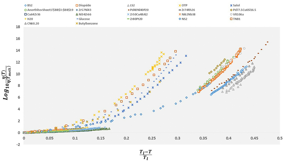
Figure 2. The viscosity, η(T), scaled by its value at the melting (or liquidus) temperature η(T_l) plotted as a function of the “reduced temperature” $\frac{{\mathit{\text{T}}}_{\mathit{\text{l}}}-\mathit{\text{T}}}{{\mathit{\text{T}}}_{\mathit{\text{l}}}}$. When represented this way, a spectrum of behaviors appears, with most glassformers seeming to fall within different “families” corresponding to fragility classes as defined by experimental values.

In light of the above arguments we will identify the cutoff temperature T_c with the melting temperature, T_m. There is an intrinsic difficulty in doing this, however, which must be addressed. Only certain non-monatomic liquids possess a single “melting” temperature. In reality, most liquids have a “melting range” associated with the temperatures between the solidus temperature T_s and the liquidus temperature T_l. Additionally, either associated with these temperatures or the pure-system melting temperature, T_m, there will be a range of energies corresponding to the latent heats/enthalpies of formation. Therefore, regardless of which temperature we choose to represent “melting,” there will be corrections necessary to account for the melting range. Additionally, many silicate systems are polymorphic in the crystalline solid state, meaning that at various temperatures below the liquidus, the crystal transitions between different thermodynamically stable crystalline configurations. These polymorphs and their associated temperatures can have a very large impact on the thermodynamic properties of the system, with minimal apparent impact on the dynamical properties. One may obtain bounds on the viscosity by setting the cutoff or melting temperature in equation (12) to mean the liquidus temperature (Nussinov, 2015). If no longtime flow appears in this intermediate temperature regime [i.e., if the terminal velocity of equation (12) vanishes], then this substitution of T_c = T_l in equations (15) and (17) will be precise. Thus, because solid-like characteristics will first appear at the liquidus temperature, we will take it to define the melting temperature at which point there is a change in the equilibrium dynamics of the system. This argument can be further understood in the context of the Lindemann criterion. In Lindemann’s model, the break down of solidity and onset of flow at the melting temperature is due to the average amplitude of vibration becoming an appreciable fraction of the lattice length (≈10%). At the temperature where this occurs, the lattice destabilizes, and constituents become liquid-like. The average amplitude of vibration is proportional to the kinetic energy, so this can be seen as the average kinetic energy of the constituents becoming enough to globally overcome the average interatomic bond strength. Observations suggest that a Lindemann-like model also holds for the devitrification of glasses (Tournier, 2016). Therefore, viewing this from the perspective of cooling, at the melting (liquidus) temperature, the “stickiness” of the interaction forces/energy first starts to dominate the kinetic energy, and the constituents begin to more strongly interact. Inserting the liquidus temperature, T_l, into equation (17), we obtain $\eta \left(T\right)=\frac{\eta \left(T_l\right)}{\mathit{erfc}\left[\frac{T_l-T}{\sqrt{2}\tilde{O}\left(T\right)}\right]}$. We next motivate a specific functional form for the distribution σ(T).

2.2. The Width of the Distribution

The spread in effective temperatures, T′, at a given external temperature, T, is quantified by σ(T). This spread (related to the variance by a simple square root) is the fundamental variable in the ESDT, as it is caused by, and leads to, the metastable, non-canonical spread in temperatures/energies. Much like the exact distribution of temperatures that it governs, we do not know a priori what its functional form should be. However, there are a number of physical constraints that will ultimately motivate its exact form. As the system is cooled, the peak of the distribution [equation (16)] shifts downward as it is centered on the external temperature, T. The tails, and not the peak, though, control how likely a macroscopic flow event will be. In order that the flow continues to decrease rapidly as the temperature is lowered, the width of the distribution will also have to shrink to “pull” the tail out of sampling the flowing states. Additionally, as the system approaches absolute zero, the third law of thermodynamics will require that the spread in energies (and hence effective temperatures) vanish, such that σ(T) must be a decreasing function of temperature. It is also readily obvious that the only natural energy scale for the metastable supercooled liquid is set by the external temperature. Therefore, it is reasonable to assume that σ(T) ∝ T. With these simple facts in mind, we assert that

$\tilde{O}\left(T\right)=\overline{A}T,$ (18)

where $\overline{A}$ is a small, dimensionless, material-dependent parameter. That is, the width σ(T) is set by the natural energy (temperature) scale of the system. Additional analysis is provided in Nussinov (2015). To confirm the validity of this approximation, we can invert equation (17) solving for the spread, σ(T), and examine it for experimental viscosity data. Across the different examined liquids, we found this to hold relatively well. In some materials, there are deviations from linearity in the vicinity of their respective solidus and/or liquidus temperatures. This is illustrated in Figure 3. As seen therein, in both glucose and supercooled water (Figure 3), σ(T) exhibits such a crossover. We found an analogous trend in supercooled salol where the crossover temperature associated with σ(T) (Weingartner et al., 2015) coincided with the earlier reported putative liquid–liquid transition temperature in this system (Mallamace et al., 2010). Similarly, supercooled water and glucose display anomalies that have been ascribed to a liquid–liquid transition (Johari et al., 1987; Mishima and Stanley, 1989; Ito et al., 1999; Tyagi and Murthy, 2006; Li et al., 2013; Murata and Tanaka, 2013; Palmer et al., 2014). Taken together, these data suggest that, if and when present, fragile to strong crossovers or liquid–liquid phase transitions (Sastry and Angell, 2003) may be associated with deviations in σ(T). This will be critically addressed in depth in a follow-up paper where we will further extensively demonstrate that $\overline{A}$ strongly correlates with various thermodynamic parameters and may allow for the prediction of low temperature viscosity from purely high temperature measurements.

FIGURE 3

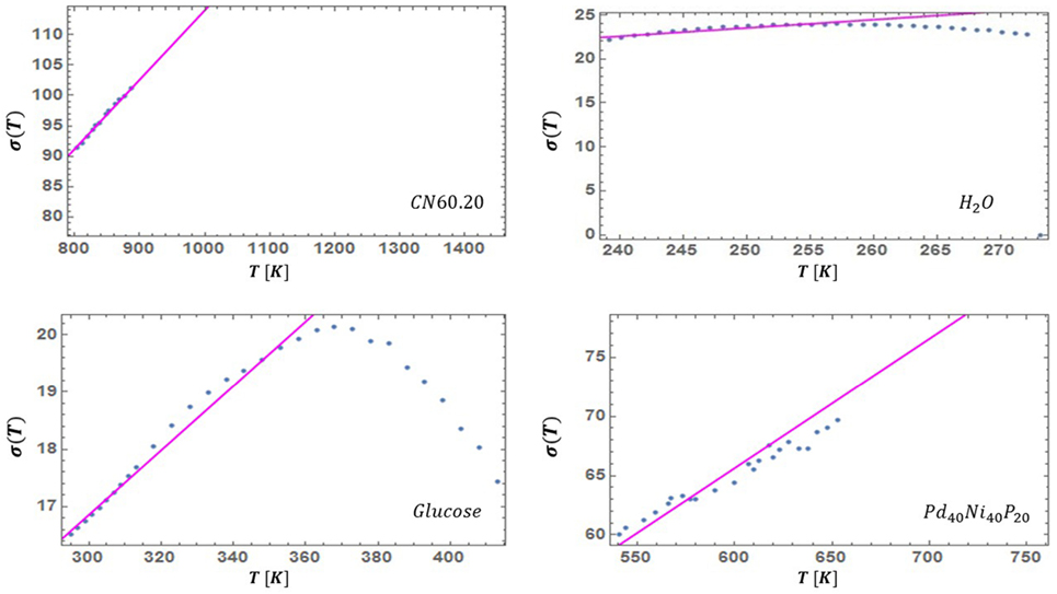
Figure 3. The SD σ(T) of the probability distribution of equation (16) as inferred by fitting the experimentally measured viscosity to equation (19). In most cases that we examined, the approximate linearity relation of equation (18) holds reasonably well far enough below the liquidus temperature. Here, we also show two well-known exceptional liquids: water and glucose. These fluids display anomalies that have been ascribed to putative liquid–liquid transitions, e.g., Johari et al. (1987), Mishima and Stanley (1989), Ito et al. (1999), Tyagi and Murthy (2006), Li et al. (2013), Murata and Tanaka (2013), and Palmer et al. (2014). The crossover of σ at high temperature and the one that we similarly found in supercooled salol (Weingartner et al., 2015) may be a signature of these putative transitions. Indeed, in salol the crossover temperature at which σ(T) deviates from its low temperature linearity (Weingartner et al., 2015) coincides with earlier experimentally suggested liquid–liquid transition temperature (Mallamace et al., 2010).

For the time being, we stress that $\overline{A}$ constitutes the only adjustable parameter in this framework. When combining this with equation (17), we now arrive, via classical phase space considerations, at our principal result for the viscosity (Nussinov, 2015),

$\eta (T)=\frac{\eta (T_l)}{\mathit{erfc}\left[\frac{T_l-T}{\sqrt{2}\overline{A}T}\right]}.$ (19)

It is immediately clear from an examination of equation (19) that our model does not possess a dynamical singularity. In fact, if one were to calculate the entropy difference between the supercooled liquid and equilibrium crystalline solid, it would be apparent that the excess entropy could only vanish at a point where the temperature distribution becomes a delta function. When this occurs, however, the system will, by definition have returned to equilibrium. Therefore, our approach makes it plain that there cannot be a finite temperature singularity, and that the above excess entropy can only vanish if the system regains equilibrium. The function of equation (19) relies only on measurable quantities associated with the liquidus and a single parameter. While the specific form of the above equation is only applicable beneath the liquidus temperature, in Weingartner et al. (2015) we derived an extension to all temperatures above the liquidus, completing the theoretical model.

A corollary of equation (19) is that the viscosity data from all supercooled liquids may be made to collapse onto one master curve (Nussinov, 2015). That is, for each fluid, the ratio of the viscosity at temperature T ≤ T_l to its viscosity at the liquidus temperature, (η(T)/η(T_l)), is a trivial function of the quotient $\left(T_l-T\right)∕\left(\overline{A}T\right)$ with $\overline{A}$ being the single dimensionless parameter that is material-dependent. We tested this prediction in Figure 4 and found it is indeed be satisfied. Although the value of $\overline{A}$ does not significantly change across all of the liquids that we examined (see Table 1), its variations are nevertheless important. In particular, it can be demonstrated that the fragility parameter is a function of both $\overline{A}$ and the reduced glass transition temperature T_rg (that are set, in our theory, by the values of the melting temperature and $\overline{A}$ themselves) (Weingartner et al., 2015). Thus, albeit being small in size, the changes in the values of $\overline{A}$ in their relatively narrow range (along with the values of T_rg) differentiate strong fluids from fragile ones. This is clearly seen in Figure 2; if the dependence on $\overline{A}$ between different glass formers were weak, the viscosity data in Figure 2 would have collapsed onto a single curve. The contrast between Figure 2 and Figure 4 (in which $\overline{A}$ was, for each liquid, set to the value given by Table 1) highlights the importance of the deviations in the parameter $\overline{A}$ (the “missing ingredient” that we alluded to above) from one fluid to another.

FIGURE 4

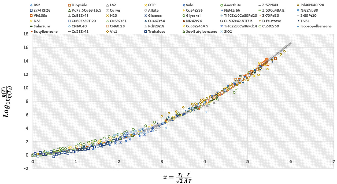
Figure 4. The viscosity data scaled by its value at the liquidus temperature, η(T_l), plotted as a function of the dimensionless temperature ratio x, as defined in the figure. The viscosity data of 45 liquids from numerous classes/bonding types (silicate, metallic, organic) and kinetic fragilities collapse onto a unique curve, suggestive of universality among all types of glass-forming liquids. Note the exceptional agreement over 16 decades. The deviations of glycerol and SiO₂ are discussed in Weingartner et al. (2015). The pertinent liquidus temperature T_l and the viscosity at T_l and our single dimensionless parameter associated with all fluids are provided in Table 1. The continuous underlying “curve” (seen at the high viscosity end where fewer viscosity data are available) is that predicted by equation (19).

TABLE 1

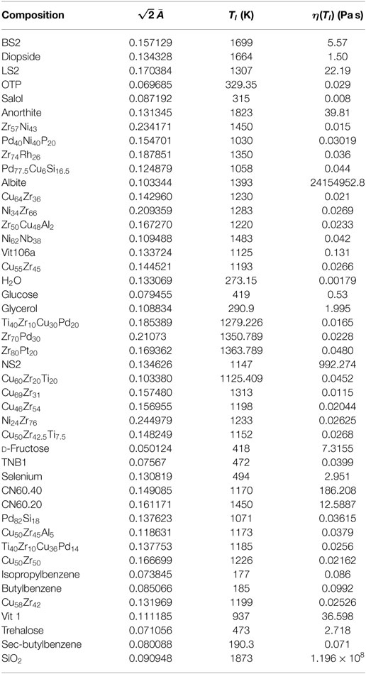
Table 1. Values of the relevant parameters of all liquids studied (equation (19)).

3. Methods: A Test of the Predicted Viscosity and a Data Collapse

With the theoretical prediction of equation (19) in hand, we now turn our attention to assessing the accuracy of the model. We examined diverse liquids belonging to both the strong and fragile classifications, and spanning all liquid types: silicate, oxide, metallic, organic, chalcogenide, sugars, and even supercooled water. We used standard non-linear fitting techniques to extract the optimal value of $\overline{A}$ for each liquid. Surprisingly, for the 45 liquids studied, the values of $\overline{A}$ fall within a narrow range (having an average and SD of 0.095 and 0.031 respectively), while simultaneously providing a visually accurate fit to the data of all studied systems. In Table 1, we list the values of $\overline{A}$ for all studied liquids and their corresponding liquidus temperatures. In Figures 5–7, we present the viscosity data of a representative sample of the supercooled liquids studied. In the figures, the solid line represents the fit of the ESDT viscosity function to the data. Visual examination of the quality of fit suggests a high degree of accuracy. To make this objective, and quantitatively rigorous, we performed a detailed statistical analysis of the data of all liquids. In Table 2, we present the results of the analysis, featuring the computed values for the sum of squared errors (SSE), reduced χ², and R² statistics for each liquid. The highest χ² values calculated (with correspondingly low R² values) correspond to glycerol and SiO₂, which appear to have anomalous behavior (Weingartner et al., 2015) and will be further addressed in detail in a follow-up paper (the melting range and bimodality likely play a role). Outside of these two liquids, the highest value of χ² is 0.7, and the lowest R² is 0.87. These results provide an objective validation of the ESDT model performance. From the combination of visual inspection and statistical analysis, it is within reason to conclude that the ESDT form for the viscosity is able to reproduce/describe the viscosity of all studied types of liquids to objectively high degrees of statistical accuracy.

FIGURE 5

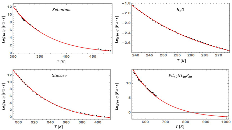
Figure 5. Fits the viscosity of various supercooled fluids (including water) with equation (19).

FIGURE 6

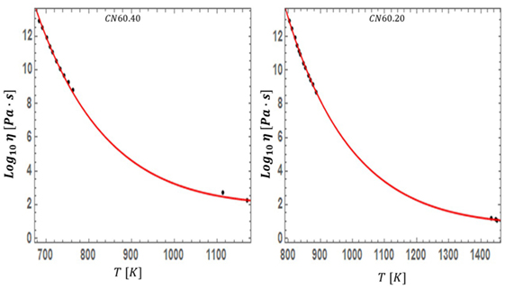
Figure 6. The fit of equation (19) is tested for CN60.40 and CN60.20, two silicate systems with slightly different molar compositions.

FIGURE 7

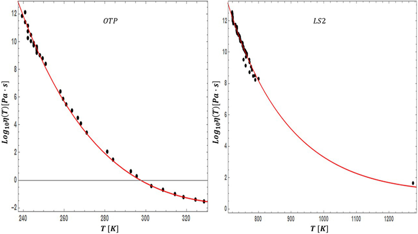
Figure 7. Our viscosity fit of equation (19) is applied to a very fragile organic glass former (OTP) and very strong silicate glass former (LS2).

TABLE 2

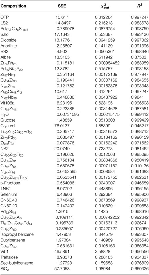
Table 2. Statistical measures of the goodness of the fit.

Whether or not the dynamics of supercooled liquids are universal has been debated for some time. We demonstrated that the ESDT viscosity form appears to fit the viscosity data of all types of supercooled liquids, thereby providing the “missing ingredient” that prevented a universal description of liquids based on melting. If the ESDT form is to be a complete picture for all liquids, then it should allow for a universal scaling of the viscosity of supercooled liquids. For that reason, we plot the logarithm of the viscosity of all studied liquids scaled by its value at the liquidus, but this time versus the argument of the complementary error function. The results of this scaling are presented in Figure 4. It is immediately clear that this scaling collapses the viscosity data of all liquid types onto a single curve. More significantly, the collapse holds over 16 decades, and for all classes/types of liquids. It should be pointed out that while this scaling arose as a consequence of the ESDT framework, even if the theoretical foundations do not hold, this scaling can always be done. While the analysis of considerably more liquids is ultimately required, this stunning result suggests that there is perhaps an underlying universality to the dynamics of all supercooled liquids.

For completeness, it must be pointed out that all liquids tested in this work undergo congruent melting and can therefore be adequately described by their liquidus temperature. There are numerous liquids, however, which undergo incongruent melting, and a small molar addition of some material can drastically change the liquidus temperature without appreciably affecting the viscosity. This is because the liquidus is where the small crystalline clusters associated with the addition will first appear, but in small enough concentrations, they cannot impact the dynamical character of the liquid. This presents a difficulty for using the liquidus as the scaling temperature for all liquids. The impact of this will be investigated in a further work but suggests that for these “pathological” liquids, a description in terms of the solidus or associated temperatures may be more appropriate.

4. Conclusion

We advanced a classical statistical mechanical framework for understanding the dynamics of supercooled liquids. We demonstrated, both qualitatively and quantitatively, that the resultant expression that is predicted by this approach [and by an earlier companion quantum version (Nussinov, 2015)] for the viscosity of supercooled liquids below the melting temperature can describe/reproduce the behavior of all liquids studied to objectively high accuracy. We demonstrated that the viscosity data of 45 different liquids can be collapsed onto a single scaling curve, suggesting that an underlying universality may be present in the dynamical behavior of supercooled liquids. Further support to our results, including data and details underlying our viscosity analysis, appears in Weingartner et al. (2015). Additional structural aspects are discussed in (Nussinov, 2015) and (Weingartner et al., 2015). We hope that our newly found universal 16 decade collapse for the viscosity data of all known liquid types and the theoretical ideas that led us to it will prompt further discussion on the underlying phenomenology of supercooled liquids and the glass transition.

Author Contributions

ZN conceived the project. NW, FN, and ZN contributed to the theory described in this work. NW gathered the data and performed the data analysis. CP and KK took the data for the various metallic liquids in their lab. NW wrote the manuscript with additions and changes from KK, FN, and ZN. All the authors were consulted at all stages of the work.

Conflict of Interest Statement

The authors declare that the research was conducted in the absence of any commercial or financial relationships that could be construed as a potential conflict of interest.

Acknowledgments

NW and ZN were supported by the NSF DMR-1411229. CP and KK were supported by the NSF DMR 12-06707, NSF DMR 15-06553, and NASA-NNX 10AU19G. ZN thanks the Feinberg foundation visiting faculty program at Weizmann Institute. The initial version of this work was completed while ZN was at the Aspen Center for Physics, which is supported by the National Science Foundation grant PHY-1066293. NW would like to sincerely thank Robert Ashcraft and Rongrong Dai for supplying data and stimulating discussions. We further thank Hajime Tanaka and Takeshi Egami for their kind words and encouragement.

References

Adam, G., and Gibbs, J. H. (1965). On the temperature dependence of cooperative relaxation properties in glass-forming liquids. J. Chem. Phys. 43, 139–146. doi: 10.1063/1.1696442

CrossRef Full Text | Google Scholar

Angell, C. A. (1995). Formation of glasses from liquids and biopolymers. Science 267, 1924–1935. doi:10.1126/science.267.5206.1924

PubMed Abstract | CrossRef Full Text | Google Scholar

Angell, C. A. (2008). Glass-formers and viscous liquid slowdown since David Turnbull: enduring puzzles and new twists. MRS Bull. 33, 544–555. doi:10.1557/mrs2008.108

CrossRef Full Text | Google Scholar

Angell, C. A., Ngai, K. L., McKenna, G. B., McMillan, P. F., and Martin, S. W. (2000). Relaxation in glassforming liquids and amorphous solids. J. Appl. Phys. 88, 3113. doi:10.1063/1.1286035

CrossRef Full Text | Google Scholar

Bengtzelius, U., Gotze, W., and Sjoilander, A. (1984). Dynamics of supercooled liquids and the glass transition. J. Phys. C 17, 5915–5934. doi:10.1088/0022-3719/17/33/005

CrossRef Full Text | Google Scholar

Berthier, L., and Biroli, G. (2011). Theoretical perspective on the glass transition and amorphous materials. Rev. Mod. Phys. 83, 587–645. doi:10.1103/RevModPhys.83.587

CrossRef Full Text | Google Scholar

Berthier, L., and Ediger, M. D. (2016). Facets of glass physics. Phys. Today 69, 40. doi:10.1063/PT.3.3052

CrossRef Full Text | Google Scholar

Blodgett, M., Egami, T., Nussinov, Z., and Kelton, K. F. (2015). Proposal for universality in the viscosity of metallic liquids. Sci. Rep. 5, 13837. doi:10.1038/srep13837

PubMed Abstract | CrossRef Full Text | Google Scholar

Cavagna, A. (2009). Supercooled liquids for pedestrians. Phys. Rep. 476, 51. doi:10.1016/j.physrep.2009.03.003

CrossRef Full Text | Google Scholar

Cohen, M. H., and Grest, G. S. (1979). Liquid-glass transition, a free-volume approach. Phys. Rev. B 20, 1077–1098. doi:10.1103/PhysRevB.20.1077

CrossRef Full Text | Google Scholar

Cohen, M. H., and Turnbull, D. (1959). Molecular transport in liquids and glasses. J. Chem. Phys. 31, 1164–1169. doi:10.1063/1.1730566

CrossRef Full Text | Google Scholar

Donati, C. J., Douglas, J. F., Kob, W., Plimpton, S. J., Poole, P. H., and Glotzer, S. C. (1998). Stringlike cooperative motion in a supercooled liquid. Phys. Rev. Lett. 80, 2338–2341. doi:10.1103/PhysRevLett.80.2338

CrossRef Full Text | Google Scholar

Ediger, M. D. (2000). Spatially heterogeneous dynamics in supercooled liquids. Annu. Rev. Phys. Chem. 51, 99–128. doi:10.1146/annurev.physchem.51.1.99

PubMed Abstract | CrossRef Full Text | Google Scholar

Elmatad, Y. S., Chandler, D., and Garrahan, J. P. (2009). Corresponding states of structural glass formers. J. Phys. Chem. B 113, 5563–5567. doi:10.1021/jp810362g

PubMed Abstract | CrossRef Full Text | Google Scholar

Elmatad, Y. S., Jack, R. L., Chandler, D., and Garrahan, J. P. (2010). Finite-temperature critical point of a glass transition. Proc. Natl. Acad. Sci. U.S.A. 107, 12793–12798. doi:10.1073/pnas.1006306107

PubMed Abstract | CrossRef Full Text | Google Scholar

Fulcher, G. S. (1925). Analysis of recent measurements of the viscosity of glasses. J. Am. Ceram. Soc. 8, 339–355. doi:10.1111/j.1151-2916.1925.tb16731.x

CrossRef Full Text | Google Scholar

Gebremichael, Y., Schroder, T. B., Starr, F. W., and Glotzer, S. C. (2001). Spatially correlated dynamics in a simulated glass-forming polymer melt: analysis of clustering phenomena. Phys. Rev. E Stat. Nonlin. Soft Matter. Phys. 64, 051503. doi:10.1103/PhysRevE.64.051503

PubMed Abstract | CrossRef Full Text | Google Scholar

Gotze, W. (2008). Complex Dynamics of Glass-Forming Liquids: A Mode-Coupling Theory. Oxford: Oxford University Press.

Google Scholar

Greer, A. L., and Ma, E. (2007). Bulk metallic glasses: at the cutting edge of metals research. MRS Bull. 32, 611. doi:10.1557/mrs2007.121

CrossRef Full Text | Google Scholar

Guggenheim, E. A. (1945). The principle of corresponding states. J. Chem. Phys. 13, 253. doi:10.1063/1.1724033

CrossRef Full Text | Google Scholar

Gupta, P. K. (1996). Non-crystalline solids: glasses and amorphous solids. J. Non Cryst. Solids 195, 158–164. doi:10.1016/0022-3093(95)00502-1

CrossRef Full Text | Google Scholar

Hancock, B. C., and Parks, M. (2000). What is the true solubility advantage for amorphous pharmaceuticals? Pharm. Res. 17, 397–404. doi:10.1023/A:1007516718048

PubMed Abstract | CrossRef Full Text | Google Scholar

Hunter, G. L., and Weeks, E. R. (2011). The physics of the colloidal glass transition. Rep. Prog. Phys. 75, 066501. doi:10.1088/0034-4885/75/6/066501

CrossRef Full Text | Google Scholar

Ito, K., Moynihan, C. T., and Angell, C. A. (1999). Thermodynamic determination of fragility in liquids and a fragile-to-strong liquid transition in water. Nature 398, 492–495. doi:10.1038/19042

CrossRef Full Text | Google Scholar

Johari, G. P., Hallbrucker, A., and Mayer, E. (1987). The glass-liquid transition of hyperquenched water. Nature 330, 552–553. doi:10.1038/330552a0

CrossRef Full Text | Google Scholar

Kalogeras, I. M., and Hagg Lobland, H. E. (2012). The nature of the glassy state: structure and glass transitions. J. Mater. Educ. 34, 69–94.

Google Scholar

Kanno, H. (1981). A simple derivation of the empirical rule T_G/T_M = 2/3. J. Non Cryst. Solids 44, 409–413. doi:10.1016/0022-3093(81)90047-8

CrossRef Full Text | Google Scholar

Kauzmann, W. (1948). The nature of the glassy state and the behavior of liquids at low temperatures. Chem. Rev. 43, 219–256. doi:10.1021/cr60135a002

CrossRef Full Text | Google Scholar

Kirkpatrick, T. R., Thirumalai, D., and Wolynes, P. G. (1989). Scaling concepts for the dynamics of viscous liquids near an ideal glassy state. Phys. Rev. A 40, 1045–1054. doi:10.1103/PhysRevA.40.1045

CrossRef Full Text | Google Scholar

Kivelson, D., Kivelson, S. A., Zhao, X., Nussinov, Z., and Tarjus, G. (1995). A thermodynamic theory of supercooled liquids. Physica A 219, 27–38. doi:10.1016/0378-4371(95)00140-3

CrossRef Full Text | Google Scholar

Kob, W. C., Donati, C., Plimpton, S. J., Poole, P. H., and Glotzer, S. C. (1997). Dynamical heterogeneities in a supercooled Lennard-Jones liquid. Phys. Rev. Lett. 79, 2827–2830. doi:10.1103/PhysRevLett.79.2827

CrossRef Full Text | Google Scholar

Langer, J. S. (2014). Theories of glass formation and the glass transition. Rep. Prog. Phys. 77, 042501. doi:10.1088/0034-4885/77/4/042501

PubMed Abstract | CrossRef Full Text | Google Scholar

Leutheusser, E. (1984). Dynamical model of the liquid-glass transition. Phys. Rev. A 29, 2765–2773. doi:10.1103/PhysRevA.29.2765

CrossRef Full Text | Google Scholar

Li, Y., Li, J., and Wang, F. (2013). Liquid-liquid transition in supercooled water suggested by microsecond simulations. Proc. Natl. Acad. Sci. U.S.A. 110, 12209–12212. doi:10.1073/pnas.1309042110

PubMed Abstract | CrossRef Full Text | Google Scholar

Lubchenko, V., and Wolynes, P. G. (2007). Theory of structural glasses and supercooled liquids. Annu. Rev. Phys. Chem. 58, 235–266. doi:10.1146/annurev.physchem.58.032806.104653

PubMed Abstract | CrossRef Full Text | Google Scholar

Mallamace, F., Branca, C., Corsaro, C., Leone, N., Spooren, J., Chen, S., et al. (2010). Transport properties of glass-forming liquids suggest that dynamic crossover temperature is as important as the glass transition temperature. Proc. Natl. Acad. Sci. U.S.A. 107, 22457–22462. doi:10.1073/pnas.1015340107

PubMed Abstract | CrossRef Full Text | Google Scholar

Mauro, J. C. (2011). Through a glass, darkly: dispelling three common misconceptions in glass science. Int. J. Appl. Glass Sci. 2, 245–261. doi:10.1111/j.2041-1294.2011.00069.x

CrossRef Full Text | Google Scholar

Mauro, J. C., Yue, Y., Ellison, A. J., Gupta, P. K., and Allan, D. C. (2009). Viscosity of glass-forming liquids. Proc. Natl. Acad. Sci. U.S.A. 106, 19780–19784. doi:10.1073/pnas.0911705106

PubMed Abstract | CrossRef Full Text | Google Scholar

Mishima, O., and Stanley, H. E. (1989). Decompression-induced melting of ice IV and the liquid-liquid transition in water. Nature 392, 164–168. doi:10.1038/32386

CrossRef Full Text | Google Scholar

Murata, K.-I., and Tanaka, H. (2013). General nature of liquid-liquid transition in aqueous organic solutions. Nat. Commun. 4, 2844. doi:10.1038/ncomms3844

PubMed Abstract | CrossRef Full Text | Google Scholar

Na, J. H., Demetriou, M. D., Floyd, M., Hoff, A., Garrett, G. R., and Johnson, W. L. (2014). Compositional landscape for glass formation in metal alloys. Proc. Natl. Acad. Sci. U.S.A. 111, 9031–9036. doi:10.1073/pnas.1407780111

PubMed Abstract | CrossRef Full Text | Google Scholar

Nishimori, H., and Ortiz, G. (2010). Elements of Phase Transitions and Critical Phenomena, Oxford Graduate Texts. Oxford University Press.

Google Scholar

Nussinov, Z. (2004). Avoided phase transitions and glassy dynamics in geometrically frustrated systems and non-Abelian theories. Phys. Rev. B 69, 014208. doi:10.1103/PhysRevB.69.014208

CrossRef Full Text | Google Scholar

Nussinov, Z. (2015). A One Parameter Fit for Glassy Dynamics as a Quantum Corollary of the Liquid to Solid Transition. Available at: https://arxiv.org/pdf/1510.03875.pdf

Google Scholar

Okui, N. (1990). Relationships between melting temperature, maximum crystallization temperature and glass transition temperature. Polymer 31, 92–94. doi:10.1016/0032-3861(90)90355-3

CrossRef Full Text | Google Scholar

Palmer, J. C., Martelli, F., Liu, Y., Car, R., Panagiotopoulos, A. Z., and Debenedetti, P. G. (2014). Metastable liquid-liquid transition in a molecular model of water. Nature 510, 385–388. doi:10.1038/nature13405

PubMed Abstract | CrossRef Full Text | Google Scholar

Parisi, G., and Mezard, M. (1999). A first principle computation of the thermodynamics of glasses. J. Chem. Phys. 111, 1076–1095. doi:10.1063/1.479193

CrossRef Full Text | Google Scholar

Procaccia, I. (2009). Physics of amorphous solids: their creation and their mechanical properties. Eur. Phys. J. Spec. Top. 178, 81–122. doi:10.1140/epjst/e2010-01184-4

CrossRef Full Text | Google Scholar

Pyrak-Nolte, L. J., and Nolte, D. D. (2016). Approaching a universal scaling relationship between fracture stiffness and fluid flow. Nat. Commun. 7, 10663. doi:10.1038/ncomms10663

PubMed Abstract | CrossRef Full Text | Google Scholar

Richert, R. (2002). Heterogeneous dynamics in liquids: fluctuations in space and time. J. Phys. Condens. Matter 14, R703–R738. doi:10.1088/0953-8984/14/23/201

CrossRef Full Text | Google Scholar

Sakka, S., and Mackenzie, J. D. (1971). Relation between apparent glass transition temperature and liquids temperature for inorganic glasses. J. Non Cryst. Solids 6, 145–162. doi:10.1016/0022-3093(71)90053-6

CrossRef Full Text | Google Scholar

Sastry, S., and Angell, C. A. (2003). Liquid-liquid phase transition in supercooled silicon. Nat. Mater. 2, 739–743. doi:10.1038/nmat994

PubMed Abstract | CrossRef Full Text | Google Scholar

Sausset, F., Biroli, G., and Kurchan, J. (2010). Do solids flow? J. Stat. Phys. 140, 718–727. doi:10.1007/s10955-010-0006-9

CrossRef Full Text | Google Scholar

Sillescu, H. (1999). Heterogeneity at the glass transition: a review. J. Non Cryst. Solids 43, 81–108.

Google Scholar

Stanley, H. E. (1999). Scaling, universality, and renormalization: three pillars of modern critical phenomena. Rev. Mod. Phys. 71, S358. doi:10.1103/RevModPhys.71.S358

CrossRef Full Text | Google Scholar

Tammann, G., and Hesse, W. Z. (1926). The dependancy of viscosity on temperature in hypothermic liquids. Z. Anorg. Allg. Chem. 156, 245. doi:10.1002/zaac.19261560121

CrossRef Full Text | Google Scholar

Tarjus, G., Kivelson, S. A., Nussinov, Z., and Viot, P. (2005). The frustration-based approach of supercooled liquids and the glass transition: a review and critical assessment. J. Phys. Condens. Matter 17, R1143–R1182. doi:10.1088/0953-8984/17/50/R01

CrossRef Full Text | Google Scholar

Telford, M. (2004). The case for bulk metallic glass. Mater. Today 7, 36–43. doi:10.1016/S1369-7021(04)00124-5

CrossRef Full Text | Google Scholar

Tournier, R. F. (2016). Lindemann’s rule applied to the melting of crystals and ultra-stable glasses. Chem. Phys. Lett. 651, 198–202. doi:10.1016/j.cplett.2016.03.043

CrossRef Full Text | Google Scholar

Turnbull, D. (1969). Under what conditions can a glass be formed? Contemp. Phys. 10, 473–488. doi:10.1080/00107516908204405

CrossRef Full Text | Google Scholar

Tyagi, M., and Murthy, S. S. (2006). Dynamics of water in supercooled aqueous solutions of glucose and poly(ethylene glycol)s as studied by dielectric spectroscopy. Carbohydr. Res. 341, 650–662. doi:10.1016/j.carres.2006.01.006

PubMed Abstract | CrossRef Full Text | Google Scholar

Uhlmann, D. R. (1972). A kinetic treatment of glass formation. J. Non Cryst. Solids 7, 337–348. doi:10.1016/0022-3093(72)90269-4

CrossRef Full Text | Google Scholar

Vogel, H. (1921). The temperature dependence law of the viscosity of fluids. Physikal. Zeitschr. 22, 645–646.

Google Scholar

Wang, L. M., Angell, C. A., and Richert, R. (2006). Fragility and thermodynamics in nonpolymeric glass-forming liquids. J. Chem. Phys. 125, 74505–74505. doi:10.1063/1.2244551

PubMed Abstract | CrossRef Full Text | Google Scholar

Weingartner, N. B., Pueblo, C., Nogueira, F. S., Kelton, K. F., and Nussinov, Z. (2015). A Quantum Theory of the Glass Transition Suggests Universality amongst Glass Formers. Available at: https://arxiv.org/pdf/1512.04565.pdf

Google Scholar

West, G. B., and Brown, J. H. (2005). The origin of allometric scaling laws in biology from genomes to ecosystems: towards a quantitative unifying theory of biological structure and organization. J. Exp. Biol. 208, 1575. doi:10.1242/jeb.01589

PubMed Abstract | CrossRef Full Text | Google Scholar

Wuttig, M., and Yamada, N. (2007). Phase-change materials for rewriteable data storage. Nat. Mater. 6, 824–832. doi:10.1038/nmat2077

PubMed Abstract | CrossRef Full Text | Google Scholar

Yue, Y. (2009). The iso-structural viscosity, configurational entropy and fragility of oxide liquids. J. Non Cryst. Solids 355, 737–744. doi:10.1016/j.jnoncrysol.2009.01.032

CrossRef Full Text | Google Scholar

Zallen, R. (1983). “The formation of amorphous solids,” in The Physics of Amorphous Solids. John Wiley & Sons, Inc., 23–32.

Google Scholar

Zhao, J., Simon, S. L., and McKenna, G. B. (2013). Using 20-million-year-old amber to test the super-Arrhenius behaviour of glass-forming systems. Nat. Commun. 4, 1783. doi:10.1038/ncomms2809

PubMed Abstract | CrossRef Full Text | Google Scholar