Connections Between Topology and Macroscopic Mechanical Properties of Three-Dimensional Open-Pore Materials

Introduction

The mechanical properties of materials with interconnected open-porous structures can be tuned by the choice of the material, the pore fraction, and the connectivity of the solid fraction. Such materials include open-pore foams (Gibson and Ashby, 1997; Ashby et al., 2000), nanoporous metals (Biener et al., 2006, 2007; Balk et al., 2009; Weissmüller et al., 2009), and architectured meta-materials (Jang et al., 2013; Zheng et al., 2014). Nanoporous Gold (NPG), with its fascinating mechanical and functional properties, has recently received significant attention due to the advances in materials development, allowing the production of specimen of mm size containing billions of nanoscaled ligaments. This material exhibits a bi-continuous network of nanoscale pores and solid “ligaments”, which are connected in nodes. Hence, it serves as an ideal model material for the investigation of structure-property relationships of open-porous materials in general.

Continuum micromechanics models including the Self Consistent Method and the Mori-Tanaka Model allow for an efficient prediction of the effective elastic properties of composites for given phase moduli and volume fractions. For a survey, see (Zaoui, 2002). To a certain extent, such models can predict the effective properties when the inclusions are pores. For example, Scheiner et al. (2016) extended this micromechanics concept to predict the micro–macro relations in the double-porous medium of hierarchically organized physiological bone and validated the model for a porosity of 10%. Motivated by the limitation to small pore fractions and homogeneity of the microstructure, Gong et al. (2011) extended the Mori–Tanaka model for porous materials of finite size. However, also such extended micromechanics models predict non-zero effective properties for porosities close to 100%. Furthermore, they assume that the entire solid fraction is bearing load.

The solid fraction φ is used as the major parameter in several theoretical models for predicting the macroscopic mechanical behavior of the porous materials (Roberts and Garboczi, 2002; Sun et al., 2013; Huber et al., 2014; Pia and Delogu, 2015; Mangipudi et al., 2016). The Gibson–Ashby model (Gibson and Ashby, 1997) is the commonly used basis for all these models. In what follows, E_s and σ_ys denote the Young's modulus and yield stress of the solid phase. The scaling of the macroscopically effective values of Young's modulus E and yield stress σ_y is dependent on the solid fraction φ in the form:

$\begin{array}{ll}\frac{E}{E_s}=C_E{\phi }^{n_E},& (1)\end{array}$

$\begin{array}{ll}\frac{{\sigma }_y}{{\sigma }_{ys}}=C_{\sigma }{\phi }^{n_{\sigma }}.& (2)\end{array}$

As summarized by Ashby and Bréchet (2003), for bending-dominated behavior, we have n_E = 2 and $n_{\sigma }=\frac{3}{2}$, while for tension-dominated behavior, n_E = n_σ = 1. An extension of the Gibson–Ashby scaling law for Young's modulus was proposed by Roberts and Garboczi (2002), who computed the density and microstructure dependent on Young's modulus and Poisson's ratio for four different isotropic random models. The data for the low-coordination number node-bond model (0.03 ≤ φ ≤ 0.3) were found to be well-described by the Gibson–Ashby scaling law Equation (1), with n_E = 2. For high densities, an equation with three parameters is suggested

$\begin{array}{ll}\frac{E}{E_s}=C{\left(\frac{\phi -{\phi }^P}{1-{\phi }^P}\right)}^m,& (3)\end{array}$

where φ = ρ/ρ_s is the solid fraction of the material. The fitting parameters φ^P = −0.0056 and m = 2.12, determined for the simulation data, can be interpreted as the percolation threshold and exponent.

Soyarslan et al. (2018) used Equation (3) to fit data computed from 3D Representative Volume Elements (RVE) of nanoporous microstructures. The RVEs are obtained using Cahn's method of generating a Gaussian random field by taking a superposition of standing sinusoidal waves that have fixed wavelength but are random in direction and phase. From the data for the macroscopic elastic modulus of the RVE for varying solid fraction, the percolation threshold for the random field microstructures is computed to be φ^P = 0.159 with an exponent of m = 2.56. Moreover, it was found that the scaled genus per volume can be represented by an analytical expression that depends on the solid phase fraction, with its maximum value at a solid fraction of φ = 0.5 and reaching the percolation threshold at a solid fraction of φ = 0.159.

An equation very similar to Equation (3) has been proposed for modeling the macroscopic Young's modulus of porous microstructures produced by sintering (Phani and Niyogi, 1987):

$\begin{array}{ll}\frac{E}{E_0}={\left(1-\frac{p}{p_c}\right)}^f.& (4)\end{array}$

In this equation, the variables p and p_c represent the porosity and the percolation threshold, respectively. E₀ is the Young's modulus of the material free of pores E₀ = E(p = 0). In context of 3D percolation theory, the model assumes a value f = 3.75 for a cluster dominated by bond-bending forces when the dimension of the system tends to infinity for all dimensions (Sahimi, 1994, p. 185). Smaller samples and sample preparation can have a strong influence on the value of f, leading to lower values close to f = 1.2. The percolation threshold from different sources varies from 0.06 to 60 Vol% (Kováčik, 1999). The interpretation of the value of f in terms of pore geometry is discussed by Phani and Niyogi (1987) with respect to the grain morphology and pore structure of the material. They conclude that for larger values f ≈ 3, the pores deviate from the spherical shape and are interconnected to a certain extent. The lower is the value of f, the more isometric and isolated is the pore phase and vice versa. Equations (3, 4) and the exponents m and f are equivalent due to the relation between the solid fraction and the porosity

$\begin{array}{ll}\phi =1-p.& (5)\end{array}$

Experimental work, including macroscopic testing (Liu et al., 2016; Liu and Jin, 2017) and 3D FIB tomography (Hu et al., 2016; Ziehmer et al., 2016), give evidence that nanoporous metals, which can be interpreted as a network of nanosized ligaments, contain a considerable fraction of so-called dangling ligaments. They originate from pinch-off events during the coarsening of the nanoporous metal, due to atomic diffusion during heat treatment. Thus, using the solid fraction φ in Equations (1, 2) significantly overestimates the mass contributing to load transfer within the ligament network (Mameka et al., 2015; Hu et al., 2016; Liu et al., 2016; Liu and Jin, 2017). It is, therefore, proposed to make use of the effective solid fraction φ_eff, which considers only the load-bearing mass of ligaments in the network. In this case, the effective solid fraction φ_eff is determined indirectly via measurement of Young's modulus under compressive deformation, assuming Equation (1) to hold for the effective solid fraction (Liu et al., 2016; Liu and Jin, 2017; Jin et al., 2018).

For a spatial network structure with complex topological and morphological characteristics, the coordination number also plays an important role (Jinnai et al., 2001). The authors investigated 3D images of morphologies arising in an ordered-block copolymer at equilibrium and a polymer blend during spinodal decomposition. They conclude that the coordination number is particularly important with regard to the assignment of bi-continuous morphologies, since it can be used to differentiate between closely related morphologies such as gyroid and diamond. Recent works investigate the skeletons of NPG obtained from FIB tomography and artificially generated structures and similarly report that mainly triple junctions and a few percent of quadruple junctions exist (Hu et al., 2016; Mangipudi et al., 2016). It can be speculated that the average coordination number is slightly higher than 3, which would be very close to the coordination number of the Gibson–Ashby unit cell (Gibson and Ashby, 1997).

Several finite element models (FEMs) simplify the 3D open-pore structure to cubic or diamond unit cells (Nachtrab, 2011; Liu and Antoniou, 2013; Huber et al., 2014; Husser et al., 2017). Hu et al. (2016) compare the simulation results from the 3D model of their FIB tomography of NPG with that of a Gibson–Ashby structure of same solid fraction. The first FEM models built from 3D FIB tomography data were presented independently by Hu et al. (2016) and Mangipudi et al. (2016). The model of Hu et al. (2016) has been further refined by Richert and Huber (2018), who analyzed the detected ligament shapes and investigated the predictive capability of the FEM beam model in comparison to the 3D solid model of Hu et al. (2016). Soyarslan et al. (2018) used complex artificially generated structures and FEM solid modeling for validating an analytical solution that relates the solid fraction to the scaled genus density. This helps to explain the divergence of experimental and numerical data from the Gibson–Ashby scaling law for Young's modulus with decreasing solid fraction.

To investigate the effect of changing connectivity on the macroscopic properties at a constant solid fraction in a more general way, Nachtrab et al. modeled the behavior of metal foams based on a diamond structure (Nachtrab, 2011; Nachtrab et al., 2011, 2012). The reduction of the connectivity was included by splitting of nodes with a coordination of 4 into two nodes, each with a coordination of 2. This led to fibrous structures with a percolation threshold p_c close to 1. For the prediction of the mechanical properties of selected additively manufactured open-pore structures, a voxel-based FE scheme was used. This scheme is, however, computationally demanding and therefore significantly limited the number of investigated structures.

To get closer to realistic microstructures, we use RVEs that are built following the idea proposed by Huber et al. (2014), where NPG is modeled as a randomized diamond structure using beam elements. The approach allows us to define a solid fraction φ by the radius r and length l of the individual ligaments (Roschning and Huber, 2016). It is also possible to vary the ligament shape (Jiao and Huber, 2017a) and to integrate nodal masses for predicting both elastic and plastic mechanical behavior comparable to the RVE, which is built with solid elements, while maintaining the computational efficiency (Jiao and Huber, 2017b). This technique enables quantitative prediction of the macroscopic Young's modulus, Poisson's ratio, and yield strength for a large number of structures.

By mechanically deactivating randomly selected ligaments in a 3D network, pinched-off (or dangling) ligaments are systematically studied in this work for the first time. The remaining load-bearing ligaments form the mass that defines the effective solid fraction φ_eff. In this way, we can shed new light on the effect of dangling ligaments in open-pore materials and expect to gain a more general and deeper understanding of the interdependencies between the coordination number, scaled genus density, effective solid fraction, percolation threshold, and the scaling behavior of mechanical properties for 3D network structures.

Methods

If we use the notation of Equation (4), a fully connected structure consisting of a given number of cylindrical ligaments has a macroscopic Young's modulus E₀. This value, corresponding to a cut fraction ζ = 0, can be computed pointwise using FEM simulations for a given solid fraction φ, defined by the ligament radius-to-length ratio r/l, i.e., $E_0={Ê}_0(\phi )={\overline{E}}_0(r/l)$, following the approach for the diamond structure (Huber et al., 2014; Roschning and Huber, 2016; Jiao and Huber, 2017a,b).

As soon as the cut fraction ζ reaches the percolation to cluster transition, the structure breaks and the mechanical stiffness becomes zero. Consequently, we can set the porosity p in Equation (4) to be equal to the cut fraction ζ and the percolation threshold for cutting is defined by the parameter ζ_c. In a more general form, Equation (4) suggests that the macroscopic Young's modulus can be written as a multiplicative decomposition

$\begin{array}{ll}E={Ê}_0\left(\phi \right){Ê}_c\left(\zeta \right).& (6)\end{array}$

While Ê₀(φ) is well-investigated, we focus in this work on mining the relationship between Young's modulus and cut fraction Ê_c(ζ) from numerical data.

Finite Element Simulations

For all FEM simulations in this work, ABAQUS (Abaqus, 2014) was used, while the raw models were built based on the unit cells as defined in Table 1 using Patran 2017 and then modified by Python scripting. Images of the FEM models and further details are provided in Data Sheet 1, Supplementary Sections 1, 2. As a substantial extension of previous work on FEM beam models, which concentrates exclusively on the diamond lattice with coordination number of 4, the RVE beam-modeling technique (Huber et al., 2014; Roschning and Huber, 2016) is generalized in this work for structures with coordination numbers ranging from 8 (bcc), 6 (simple cubic), 4 (diamond), to 3 (Gibson–Ashby). For all structures, the bcc structure serves as reference, because in terms of the coordination number, a lower coordination can always be reached by cutting connections in a higher coordinated structure. By orienting the < 111>-direction of the cubic structure along the loading direction, all investigated structures deform by bending, which is the major deformation mechanism of NPG (Huber et al., 2014; Griffiths et al., 2017; Jiao and Huber, 2017a). In this way, it is ensured that the scaling laws for the mechanical properties are based on the same deformation mechanism.

TABLE 1

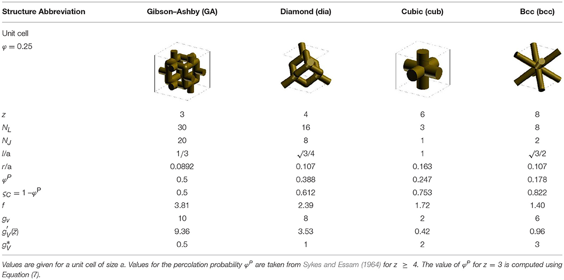
Table 1. Geometry parameters for structures with different coordination number z.

The unit cells, as described in section Unit Cell Geometries, serve as building blocks for the generation of the RVE, which is described in section RVE Generation. Motivated by the high flexibility in the model setup and computational efficiency even for large 3D networks, all following unit cells and RVEs are built using the FEM beam model approach originally developed for the diamond structure (Huber et al., 2014). This approach has been thoroughly investigated and validated in subsequent works with respect to the solid fraction and macroscopic mechanical properties for cylindrical and parabolic ligaments (Roschning and Huber, 2016; Jiao and Huber, 2017a,b). The randomization of the structure was found as an important parameter to adjust the macroscopic behavior of the structures to experimental results, particularly for calibrating the elastic Poisson's ratio (Huber et al., 2014; Roschning and Huber, 2016; Lührs et al., 2017). So far, only fully connected 3D networks have been investigated. It is, thus, of obvious interest to quantitatively investigate the effect of cutting of a fraction of connections in the ligament network.

Unit Cell Geometries

The unit cell geometries for different coordination numbers z of 3 (Gibson–Ashby or GA), 4 (diamond or dia), 6 (simple cubic or cub), and 8 (bcc) are depicted in Table 1. The number of cuts until complete decohesion of the structure can be treated as a general problem of topology. A characteristic parameter is the percolation threshold ${\zeta }_c=1-{\phi }^P$ at which the structure loses its connectivity and the macroscopic mechanical properties become zero. For most structures used in this work, the critical percolation probabilities φ^P for the “bond problem” are known (Domb and Sykes, 1961; Sykes and Essam, 1964), and the data can be summed up with a simple rule of thumb, which is valid with an accuracy of a few percent from z = 4 to z = 12 (Ziman, 1968):

$\begin{array}{ll}{1-{\zeta }_c=\phi }^P\cong \frac{1.5}{z}.& (7)\end{array}$

The data for the critical percolation probabilities φ^Pand percolation thresholds ζ_c are included in Table 1. For the Gibson–Ashby structure, which is located at the lower end of connectivity, Equation (7) predicts a value of ζ_c = 0.5.

The unit cell defines the ligament length l dependent on the unit cell size a, as seen in Table 1. The solid fraction of the fully connected structure can be calibrated to any value via the ligament radius r for each structure. For the generation of the data in section Macroscopic Mechanical Properties, a solid fraction of φ = 0.25 was used, which is a typical value for NPG (Weissmüller et al., 2009). For simplicity, the calculation of the solid volume was estimated by the total of N_L cylindrical ligaments $V_s=N_L\pi r^{2}l$, with the numbers given in Table 1. The solid fraction is adjusted such that $\phi =V_s/a^3=0.25$, ignoring overlapping volumes or gaps in the cylindrical ligaments in the nodal area.

RVE Generation

The generation of periodic RVEs from unit cells is straightforward when the RVE boundaries are aligned with the unit cell boundaries. Because the simple cubic structure would normally deform under compression in its original orientation, the periodic cubic structure was generated to be large enough that after rotating the < 111> direction into z-direction, a cube of the size of the RVE is completely filled. All ligaments penetrating the boundaries of the RVE were clipped at the boundary plane and the structure was cut to the size of the RVE.

For the fundamental investigation on the effect of cutting of 3D structures represented by the dependency Ê_c(ζ) in Equation (6), the problem can be simplified to the relevant information of connectivity. A refined modeling, considering the randomization of the structure (Huber et al., 2014; Roschning and Huber, 2016), incorporation of variable ligament shapes (Jiao and Huber, 2017a), or nodal mass using the so-called nodal-corrected beam model (NCBM) (Jiao and Huber, 2017b) are related to the dependency Ê₀(φ) in Equation (6). This is set aside for generating more realistic structures for validation in section Randomized Diamond Structures With Nodal Correction. For details on the generation of such RVEs, please refer to Data Sheet 1 in the Supplementary Section 1.

In the diamond structure (Huber et al., 2014; Roschning and Huber, 2016), the boundary conditions are chosen as symmetry conditions applied to the nodes in the planes x = 0, y = 0, and z = 0. The load is applied as a homogeneous displacement of all nodes on the top side of the RVE, applying a compressive strain of maximum 15%. To capture the boundary conditions of a uniaxial compression experiment, all nodes on the remaining faces are free to move. For the mechanical properties of the solid fraction, Young's modulus E_s = 80 GPa, Poisson's ratio ν = 0.42, yield strength of σ_{y, s} = 500 MPa, and work-hardening rate of E_T = 1000 MPa were chosen. These parameters represent the mechanical behavior of the ligaments in NPG reasonably well (Huber et al., 2014; Hu et al., 2016; Roschning and Huber, 2016).

The cut fraction ζ defines the number of cut ligaments relative to the total number of ligaments in the RVE. Cutting of ligaments is realized by setting the Young's modulus for a set of FE elements, which form a randomly selected ligament, to a low value of ${E_{cut}=10}^{-3}{E}_s$. This ensures that otherwise free-floating parts of the model remain connected, despite being mechanically negligible. In this way, convergence can be achieved in the FE simulations even for structures beyond the percolation threshold. By the random removal of ligaments from a higher coordinated structure, for example, a bcc structure, it is possible to provide an initial structure that has an average coordination number equal to lower coordinated structures. For example, by removing half of the ligaments, the bcc structure is turned into a structure with the same average coordination number as the diamond structure. For more details on the data structure and data processing, please refer to Data Sheet 1 in the Supplementary Section 2.

In previous works, an RVE size of 4 × 4 × 4 unit cells was used for the fully connected diamond structure and effects of structural randomization were averaged from 5 to 10 realizations of RVEs of same size (Huber et al., 2014; Roschning and Huber, 2016; Jiao and Huber, 2017a,b). Preliminary studies on diamond structures with random cutting of ligaments show that an RVE size of 6 × 6 × 6 unit cells represents a good compromise between accuracy and computational cost, as seen in Data Sheet 1 in the Supplementary Section 3. At this size, the macroscopic Young's modulus is predicted with an accuracy of 5%, while elastic-plastic compression up to 15% strain takes 2 CPUh for a single realization. Furthermore, bcc and cubic structures serve to create representative structures with reduced coordination numbers by removing a given fraction of ligaments. For these two higher coordinated structures, the RVE size was therefore increased to 12 × 12 × 12 unit cells.

Artificial Neural Networks

Feed-forward artificial neural networks (ANN) (Haykin, 1998) are a machine-learning technique that enable the approximation of arbitrary non-linear relationships between multiple input and outputs (Yagawa and Okuda, 1996). An ANN can mathematically be represented as an operator that maps an input vector x to an output vector y

$\begin{array}{ll}\text{y}={N}\left(x,w\right).& (8)\end{array}$

The synaptic weights w of the flexible function ${N}$ are calibrated by training the ANN with patterns, consisting of pairs of input data x and desired outputs d. The training algorithm minimizes the error for all outputs and all patterns presented to the ANN during training through the iterative adjustment of the synaptic weights w. In this context, the number of training increments is called epoch. A percentage of the provided patterns (typically 10%) are kept for validation and are not used for training.

The error for a presented set of patterns is computed from the squared error for all K outputs and P patterns by the following equation:

$\begin{array}{ll}E={{\displaystyle \sum }}_{p=0}^P{{\displaystyle \sum }}_{k=0}^K{(y_k^{\left(p\right)}-d_k^{\left(p\right)})}^2.& (9)\end{array}$

Normalizing the squared error E by KP yields the mean squared error MSE, which allows the comparison of results from different pattern sizes and neural network architectures. This is helpful for comparing the prediction quality of training and validation patterns, as denoted by MSE_T and MSE_V, respectively.

Observing the development of the training and validation error during training provides important insight into whether the function ${N}$ exists and if the information in the input data x is sufficiently complete for obtaining the desired outputs d. A very limited decay of the training error indicates that the problem at hand cannot be (uniquely) solved. A decay of the training error to low values along with a significant increase in validation error indicates overlearning, which leads to lack of generalization. In this case, the ANN tends to classify and memorize each pattern individually and is not able to interpolate between the patterns. When the ANN reaches low training and validation error, it can be used to predict the output for any input, provided that the data are within the training range of the ANN. For details about the ANN simulation software and its application to various problems in mechanics and materials science please refer to Huber et al. (2002), Tyulyukovskiy and Huber (2006), Tyulyukovskiy and Huber (2007), Willumeit et al. (2013), and Chupakhin et al. (2017).

Macroscopic Mechanical Properties

This section addresses the general question as to whether a relationship exists between cut fraction and macroscopic mechanical properties and if so, how this relationship can be represented. This type of problem can be addressed by data mining. In addition, there are a number of specific questions. The literature suggests that the behavior of the mechanical properties follows a power-law behavior, as given in Equation (4). It is unclear whether the values for the percolation threshold from literature collected in Table 1, which were computed for the fundamental problems of ferromagnetic crystals and electron transport, can be transferred to our solid mechanics context.

Sykes and Essam (1964) propose Equation (7) for computing the percolation probability from the coordination numbers ranging from 4 to 12 with only a few percent error. The open question is how accurate this rule of thumb is for values below 4. If it still describes the overall dependency sufficiently well, we could speculate that once the average coordination number of a 3D network reaches a value of 1.5, there is no further cut possible without losing connectivity. This value appears to be surprisingly low.

Study of Percolation Behavior

In this section, the behavior of the macroscopic Young's modulus and yield strength are studied for initially fully connected structures, as listed in Table 1, by varying the cut fraction ζ in 10% increments. The macroscopic Young's modulus was computed from the response of the RVE after the first loading increment, which is fully elastic. To determine the yield strength, the corresponding plastic strain was computed at each load increment and the macroscopic stress-plastic strain curve was interpolated to 0.2% of plastic strain. The results for the different structures under investigation are shown in Figure 1, normalized to the value of the corresponding fully connected structure. The scatter of five realizations for each cut fraction is visible from the symbols, representing the individual numerical results.

FIGURE 1

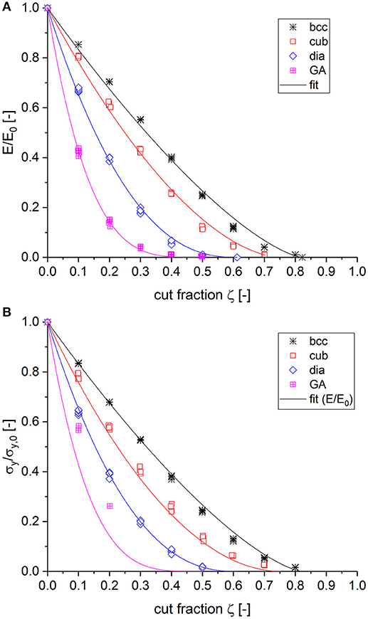
Figure 1. Decay of macroscopic properties dependent on the cut fraction ζ for bcc, cubic < 111> (cub), diamond (dia), and Gibson–Ashby (GA) structures. All data are normalized to the value of the fully connected structure. (A) Young's modulus and (B) yield strength.

For the normalized macroscopic Young's modulus, as shown in Figure 1A, the behavior was fitted by adjusting the exponent f in Equation (4), while the values for the percolation threshold p_c from Table 1 were inserted as a predefined parameter for the respective structure. It can be seen that the exponent f increases with decreasing coordination number. The fit results presented in Figure 1A confirm that the value of f cannot be understood as an invariant number, as suggested in literature (Sahimi, 1994). Instead, it strongly depends on the initial structure under study. For high coordination numbers, the exponent tends toward 1, while for low coordination numbers it exceeds the value of 3, confirming the findings summarized by Kováčik (1999). However, in our work, this value is not related to the extension of a pore morphology, which could be interpreted as a network of cut ligaments within the RVE, but instead it is related to the coordination number of the respective fully connected structure.

It is striking how well the very same behavior applies to the yield strength shown in Figure 1B. The fit curves determined from the Young's modulus also show strong agreement with the strength data for diamond, cubic, and bcc structures. Concerning the Gibson–Ashby structure, it is not clear if this applies here as well, because only few simulations reached sufficient plastic strains. Due to the missing statistics and the numerical issues, the few remaining data points are arguable. Irrespective of this uncertainty, the result strongly suggests that the Young's modulus and yield strength follow the very same behavior for partially cut structures.

Scaling of Mechanical Properties

The numerical experiment carried out in section Study of Percolation Behavior is based on the idea of random cutting of ligaments of an initially fully connected structure. For each type of structure, the degradation of the macroscopic mechanical properties follows a non-linear behavior that is defined by the coordination number of the corresponding fully connected structure. Following this line of thinking leads to the speculation that the behavior of a structure with a certain fraction of missing connections might be defined by the original unit cell structure.

On the other hand, simple math suggests that cutting 25% of the ligaments in a bcc structure with a coordination number z = 8, for example, yields the coordination number of the cubic structure (z = 6). The question at hand is whether the topology of a structure with higher coordination number can be effectively transformed into the topology of any structure of lower coordination number. It follows that the macroscopic properties for a given solid fraction is defined by the average coordination number via the second part of Equation (6). Ensuring a consistent scaling of mechanical properties, however, requires that the structures under consideration deform through the same mechanism. In this work, we therefore concentrate on structures that show bending as the dominant deformation mechanism (Huber et al., 2014).

Young's Modulus

The hypothesis presented in the previous paragraph is tested as follows: Starting from a fully connected bcc structure, a new starting structure is generated, in which a defined percentage of ligaments, ζ_ini are removed. The steps were chosen such that the connectivity is continuously reduced from 8 to 4 in steps of 1, i.e., ζ_ini ∈ {0, 0.125, 0.25, 0.375, 0.5}. Again, for each of these structures, the macroscopic Young's modulus was subsequently calculated, depending on the cut fraction ζ increased by 10% increments, with five random realizations for each increment. The results, analyzed according to section Study of Percolation Behavior in Data Sheet 1 (Supplementary Section 4), suggest that it should be possible to combine the data from different structures in a single curve.

To this end, the total cut fraction ζ_tot is calculated from ζ_tot = 1 − (1 − ζ_ini)(1 − ζ), where ζ is defined as the cut fraction relative to the remaining solid fraction of the pre-cut structure. All data related to the macroscopic Young's modulus E are normalized by the value computed for the fully connected bcc structure, which is denoted as E_{0, bcc}. The results for the bcc structure are compiled in Figure 2A as black crosses.

FIGURE 2

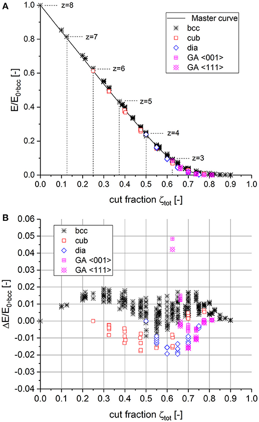
Figure 2. (A) Construction of the master curve derived from bcc data and validation with data obtained independently from fully connected cubic, diamond, and Gibson–Ashby (GA) structures. (B) Deviation between numerical data and the proposed master curve.

The curve constructed from the bcc data in Figure 2A clearly shows that the power law function Equation (4) is not capable of describing the behavior from the fully connected structure down to the percolation to cluster transition. Therefore, we suggest a function consisting of an initially linear descent for ζ_tot ≥ 0 with a sigmoidal transition toward the percolation threshold ζ_c in the following form:

$\begin{array}{l}\frac{E}{E_{0,bcc}}=Ẽ\left({\zeta }_{tot}\right)=1-a_0{\zeta }_{tot}+\frac{a_1}{\left[1+exp\left({-a}_2\left({\zeta }_{tot}-{\zeta }_c\right)\right)\right]},\\ 0\le {\zeta }_{tot}\le {\zeta }_c.& (10)\end{array}$

The parameters in Equation (10) can be adjusted to satisfy the conditions E/E_{0, bcc}|_ζc = 0 and dE/dE_{0, bcc}|_ζc = 0 by setting a₁ = 2(a₀ζ_c−1) and a₂ = 4a₀/a₁. The percolation threshold ζ_c = 0.822 is taken from Sykes and Essam (1964). Please also see Table 1 for the bcc structure. By using the literature value for infinite structure size, a treatment of the finite-size scaling effect (Sahimi, 1994; Nachtrab, 2011) in the numerical data can be avoided. This leads to a single adjustable parameter a₀, which is determined from the linear slope of the numerical data at low total cut fractions to a₀ = 1.55. It follows that a₁ = 0.55 and a₂ = 11.31.

For validation of the master curve, the data from section Study of Percolation Behavior, computed for the cubic, diamond, and Gibson–Ashby structure, are included in Figure 2A according to the following procedure. As the coordination number of the bcc structure z_bcc = 8 is used as reference, the calculation of the total cut fraction can be done in the following form

$\begin{array}{ll}{\zeta }_{tot}=1-\frac{z_x}{z_{bcc}}\left(1-{\zeta }_{ini}\right)\left(1-\zeta \right),& (11)\end{array}$

where the term z_x/z_bcc scales the current structure x with a coordination number z_x relative to that of the bcc reference structure z_bcc and defines the starting point for the total cut fraction on the master curve. Alternatively, the average coordination number $\overline{z}=z_x(1-{\zeta }_{ini})(1-\zeta )$ of an RVE can be determined by averaging the coordination number over all the internal nodes within the RVE. Incorporating nodes at boundaries would add a bias toward lower coordination numbers. The numerical data confirm the following linear relationship:

$\begin{array}{ll}\overline{z}=z_{bcc}\left(1-{\zeta }_{tot}\right).& (12)\end{array}$

This is confirmed with an accuracy of 5% for all structures under investigation. The vertical adjustment of the starting point of an initially fully connected structure x is defined by normalizing the Young's modulus data, such that the value E_{0, x}/E_{0, bcc} calculated from Equation (10) for ζ_ini = 0 and ζ = 0 is met. The corresponding values are given in Data Sheet 1, Supplementary Table 1.

Furthermore, Figure 2A includes the data for the other structures (cub, dia, GA) of Figure 1A mapped to E/E_{0, bcc} vs. ζ_tot. The overall agreement with the master curve appears to be very good. The quantitative comparison, as presented in Figure 2B, shows the deviation between the numerical data and the master curve with an error of < 2% for all structures, except for the uncut Gibson-Ashby structures showing a deviation of 5%. Although this is a factor of two and is better compared to the power law fit using Equation (4) of Figure 1A, it should be kept in mind that this accuracy is relative to the macroscopic Young's modulus E_{0, bcc} of a fully connected bcc structure with a relatively high coordination number.

Remembering the strong agreement of the macroscopic yield strength data with the fit curves for macroscopic Young's modulus presented in Figure 1B, it can be expected that the same master curve as determined for Young's modulus can be applied to the macroscopic yield strength as well. This is shown in Figure 3A for bcc structures with different degrees of initial cutting. For low cut fractions (or high coordination numbers), the yield strength data fall about 3% below the master curve. However, with increasing cut fraction (or for lower coordination numbers), the difference reduces. For ζ_tot ≥ 0.55 (z ≤ 3.6), the two properties show a perfect match.

FIGURE 3

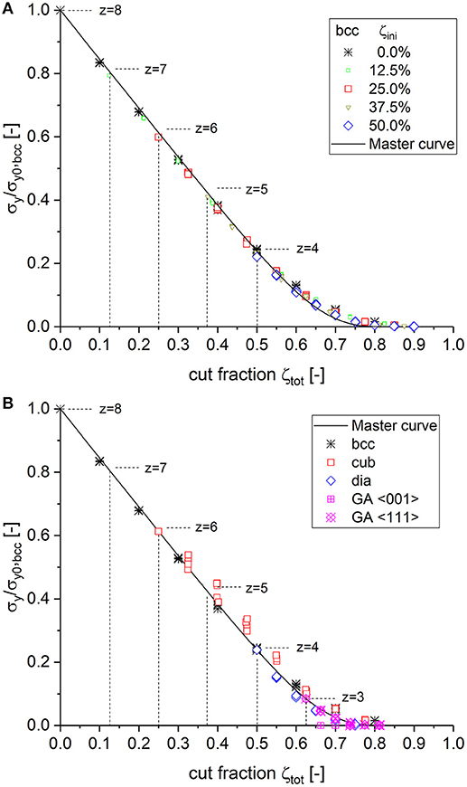
Figure 3. (A) Scaling behavior of the macroscopic yield strength as obtained from different degrees of initial cutting of bcc structures plotted together with the master curve Equation (10), using the parameters as determined for macroscopic Young's modulus. (B) Validation of the master curve with data of fully connected simple cubic (cub), diamond (dia), and Gibson–Ashby (GA) structures.

The validation carried out by using data from the structures with originally different unit cell geometry and coordination number is shown in Figure 3B. It can be seen that the scatter is larger, particularly for the cubic structure. The cubic structure is also located a few percent above the values of the other structures. It can be argued that the cubic structure is the only one in which the unit cell does not agree with the coordinate directions of the RVE boundary. Due to the rotation in < 111> direction, numerous ligaments are cut at the RVE boundary to form a cube of size 12 × 12 × 12 unit cell size. The shorter ligaments show a higher strength due to the reduced lever available for bending (Huber et al., 2014). It can therefore be concluded that σ_y/σ_{y0, bcc} = E/E_{0, bcc} = Ẽ(ζ_tot) holds within the numerical accuracy and Equation (10) can be identically applied for predicting both the scaling behavior of the macroscopic Young's modulus and the yield strength.

Poisson's Ratio

The successful construction of a master curve for the macroscopic Young's modulus and yield strength from numerical data motivates the search for a master curve for Poisson's ratio. Starting from the bcc structure with increasing fraction of initial cuts leads to the behavior shown in Figure 4A. In contrast to the behavior of the Young's modulus and yield strength, the initial slope for low total cut fractions ζ_tot ≳ 0 is close to zero and then takes progressively negative values. At ζ_tot ≳ 0.7, the data show a minimum value. The scatter strongly increases while the curve changes direction toward larger values. As the structure rapidly loses connectivity with ζ_tot → 0.822, the lateral expansion of the RVE is based on very few connections within the 3D network, causing the large scatter and the change in the overall trend. It could be speculated that Poisson's ratio should theoretically continue downwards toward zero when approaching the percolation threshold. Based on this assumption, a simple fit function with a single adjustable parameter can be formulated that assumes an elliptic shape:

$\begin{array}{ll}\frac{\nu }{{\nu }_{0,bcc}}=\tilde{\nu }\left({\zeta }_{tot}\right)={\left(1-{\left(\frac{{\zeta }_{tot}}{{\zeta }_c}\right)}^n\right)}^{1/n},0\le {\zeta }_{tot}\le {\zeta }_c.& (13)\end{array}$

The master curve for Poisson's ratio, as plotted in Figure 4A as a dashed curve, uses ζ_c = 0.822 as fixed percolation threshold for the bcc structure, similar to Equation (10), and an exponent n = 1.75.

FIGURE 4

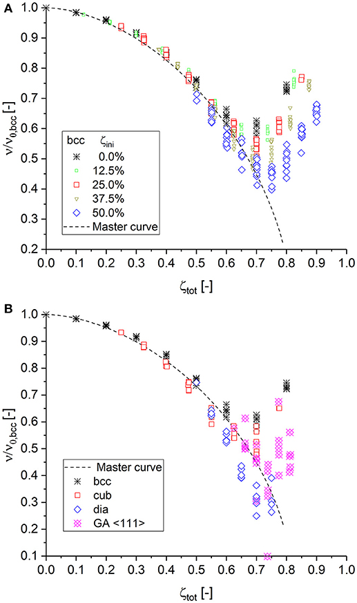
Figure 4. (A) Construction of the master curve for Poisson's ratio depending on the cut fraction based on the bcc structure with different degrees of initial cuts. (B) Validation of the master curve with data of subsequent cutting starting from fully connected cubic < 111> (cub), diamond (dia), and Gibson–Ashby (GA) structures.

In contrast to the macroscopic Young's modulus and strength, which are measured in loading direction, Poisson's ratio characterizes the lateral expansion normal to the loading direction. It is, therefore, not obvious that the master curve can also apply to structures built from very different unit cells, as their deformation mechanisms could significantly differ. However, both the simple cubic and the diamond structure agree equally well with the master curve. Interestingly, the diamond structure, which starts as fully connected structure at the low coordination number of z = 4, shows a further continuation of the downwards trend along the master curve and confirms the hypothesis that Poisson's ratio should actually continue toward zero as the percolation threshold is approached. This hypothesis is further supported through additional simulations conducted for the low coordinated Gibson–Ashby structure, loaded in < 111> direction, which are incorporated in Figure 4B.

Relationship Between Scaled Genus Density and Average Coordination Number

Throughout the previous analysis, the total cut fraction ζ_tot was used as an independent variable for the characterization of the connectivity. By this approach, common issues with determining the percolation threshold p_c and exponent could be avoided. For measuring the total cut fraction of a real structure, e.g., from a skeleton of a FIB tomography (Hu et al., 2016; Ziehmer et al., 2016; Hu, 2017; Richert and Huber, 2018), the related fully connected reference is required; however, this is unknown. Alternatively, the average coordination number $\overline{z}$ of a 3D network could be measured, because it is connected with the total cut fraction by the linear relationship, as given in Equation (12). But even if the skeleton of a structure is available, the determination of the average coordination number $\overline{z}$, as defined in this work, is difficult.

By averaging the coordination numbers of all junctions, N_z, the average coordination number $\overline{z}$ should be obtained. The problem is that any junction with fewer than three connections cannot be recognized. A junction that connects two branches is invisible because the two branches form a single longer branch. A node that has lost all connections physically reduces to a void junction, which is undetectable in any case. Thus, one would naturally obtain $\overline{z}=3$ as the lower limit, irrespective of how many more cuts are introduced in a structure. This is consistent with the results of Ioannidis and Chatzis (2000), where only pores with z ≥ 3 are considered as valid nodes in topological context. Consequently, with ongoing removal of connections, the number of detectable junctions starts to decrease at the same time.

A third parameter that is frequently used is the genus density g_V. The genus g is the maximum number of non-intersecting closed curves along which the object can be cut without dividing it into two parts (Richeson, 2008). As no internal pores are present in our structures, the genus equals the connectivity. For 3D networks consisting of solid struts, as represented by a graph G, the genus g is calculated from the Euler characteristic χ(G) = 1−g, where χ(G): = V−E, with V and E being the number of graph vertices and the number of graph edges, respectively (Nachtrab, 2011; Hu et al., 2016). Note that this calculation of the genus assumes connected structures. As we do not account for the formation of free floating clusters, this can lead to negative values of g, because the formation of clusters and the cutting of all load-bearing rings may happen before reaching the percolation threshold.

Because the genus increases with increasing structure size, it is commonly scaled to a characteristic volume, g_V = g/V_c. To compare the topology of different structures, the dimensionless product $g_V{S}_V^{-3}$ is used. In the context of nanoporous metals, 1/S_V is typically chosen as characteristic length, representing the reciprocal of the interfacial area per volume of a given system (Kwon et al., 2010). This definition can be applied to 3D solid structures with an interface separating the solid fraction and the pore space, for which all characteristic lengths are linearly dependent due to the geometrical similarity of the structure under investigation (Kwon et al., 2010; Hu et al., 2016; Mangipudi et al., 2016; Hu, 2017). Therefore, the importance of the characteristic length scale for the normalization and the associated challenges in its experimental determination are still under debate (Lilleodden and Voorhees, 2018).

The large data set for various structures sheds some light onto this. The way in which the structures have been generated in this work enables the setting of any arbitrarily chosen value for the ligament radius, independent of the topology of the structure. Consequently, the interfacial area is fully decoupled from the genus, which is in contrast to the approach of generating artificial nanoporous structures based on the Cahn–Hilliard equation (Kwon et al., 2010; Sun et al., 2013; Mangipudi et al., 2016; Soyarslan et al., 2018). Moreover, Soyarslan et al. (2018) could show for this type of structures that the solid fraction controls the scaled genus density and a closed form relationship exists that uniquely relates the two quantities to each other.

By using the large set of data for structures covering a large range of coordination numbers and cut fractions, we are able to determine which characteristic length, more generally denoted as l_V, allows the transfer of results for the scaled genus density among the different structures. For comparing RVEs of different sizes, all results are normalized by the number of unit cells in the model, i.e., $g_V=(1-\chi (RVE))/N^3$, where N = 12 for all bcc- and cubic-based structures, and N = 6 for all diamond- and Gibson–Ashby-based structures. The results for g_V are plotted in Figure 5A. All curves intersect at g_V = 0, which indicates that the genus is correctly calculated, as this particular point should be common for all structures, independent of the scaling. The data suggest that the intersection with g_V = 0 corresponds to an average coordination number z ≲ 2. Below this point, i.e., for g_V < 0, clusters form and the mechanical properties are zero. For $\overline{z}>2$, the curves $g_V(\overline{z})$ separate because the different unit cells have a different genus, as seen in Table 1.

FIGURE 5

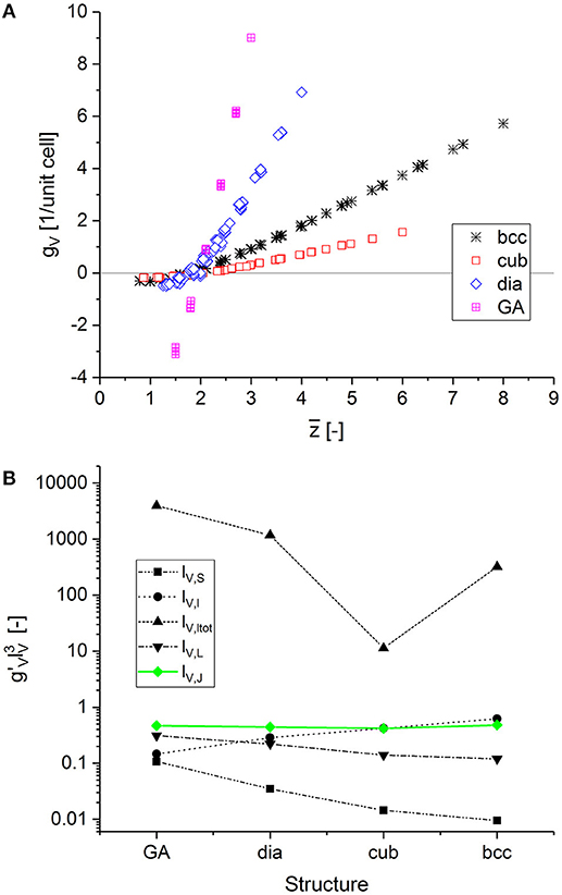
Figure 5. Calculated scaled genus density plotted vs. average coordination number for different structures and cut fractions: (A) genus per unit cell volume vs. average coordination number. (B) fingerprint of various definitions for the characteristic length l_V with the condition $g_V^{\prime }{l}_V^3=const$ fulfilled only for the characteristic length l_V,J (green).

We can now derive a fingerprint from the data in Figure 5A, which supports the search for the characteristic length l_V. Following Kwon et al. (2010), the scaled genus density $g_V(\overline{z})$ is defined as

$\begin{array}{ll}{g}_V^{*}\left(\overline{z}\right):=g_V\left(\overline{z}\right)l_V^3.& (14)\end{array}$

As long as the structures under investigation are self-similar, any characteristic length $l_V^3$ can be chosen, such as 1/S_V or the ligament diameter 〈D〉 (Hu et al., 2016). However, when the self-similarity is no longer conserved, we need to select a characteristic length that works for all structures. Our data set supports the search for l_V to fulfil the condition $g_V^{*}(\overline{z})=const$, independent of the structure. As can be seen in Figure 5A, g_V depends linearly on $\overline{z}$ in the upper right area of the plot. In this region, the condition $g_V^{*}(\overline{z})=const$ can be replaced by $g_V^{*}{ }^{\prime }=g_V^{\prime }{l}_V^3=const$. The slopes $g_V^{\prime }$ characterizing $g_V(\overline{z})>$1 are listed in Table 1.

A number of possible characteristic lengths l_V can be obtained from the geometrical parameters defining the structure of the different unit cells, such as the coordination number z, the ligament length l, the ligament radius r, the number of ligaments per unit cell N_L, and the number of junctions per unit cell N_J. We can exclude the coordination number z as the independent variable, as well as combinations with the ligament radius r for the aforementioned reasons. As one example of this category of characteristic lengths, the inverse of the ratio of surface area by volume is tested. Normalizing the unit cell volume by the surface area of the cylindrical ligaments in the unit cell, we can estimate $S_V^{-1}\text{ by }{l}_{V,S}:=a^3/(N_{L}2\pi rl)$. The other characteristic lengths are the ligament length l_V,l: = l, the total ligament length in the unit cell, l_V,ltot: = N_Ll, and characteristic lengths calculated from the volume per junction and from the volume per ligament, as $l_{V,J}:={(a^3/N_J)}^{1/3}$ and $l_{V,L}:={(a^3/N_L)}^{1/3}$, respectively.

The dependency of $g_V^{\prime }{l}_V^3$ for the different definitions of l_V plotted in Figure 5B reveals that only the characteristic length l_V,J satisfies the condition $g_V^{\prime }{l}_V^3=const$. If this is inserted in Equation (14), we get

$\begin{array}{ll}{g}_V^{*}\left(\overline{z}\right):=\frac{g\left(\overline{z}\right)}{N^3{N}_J}=\frac{g\left(\overline{z}\right)}{N_{J,RVE}}.& (15)\end{array}$

Therefore, the definition of a scaled genus density, which combines all structures in a single curve, requires a normalization of the genus by the number of junctions of the original, fully connected structure, N_J,RVE, given by the number of unit cells in the RVE, N³, multiplied by the number of junctions per unit cell, N_J. This finding is consistent with Ioannidis and Lang (1998) and Ioannidis and Chatzis (2000), where the genus per node was used.

By knowing the characteristic length for scaling the genus density, we can derive a closed form relationship for $g_V^{*}$ depending on the RVE size N, which can be analyzed for any unit cell, as seen in Data Sheet 1, Supplementary Section 5. The results shown in Figure 6A reveal that structures with a scaled genus density that is sufficiently insensitive to the surface require an RVE size in the order of 100. Thus, the relationship $g_V^{*}(\overline{z})$ that holds for large structures should be determined from the analytical solution for the infinite RVE size. To confirm this approach, the numerical and analytical data are plotted in Figure 6B. The strong agreement for RVE sizes of 6 to 12 with corresponding curves for finite structure size validates the analytical solution provided in Supplementary Equations (9–14) in Data Sheet 1.

FIGURE 6

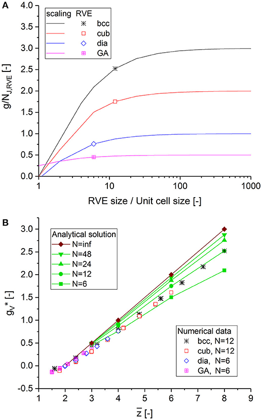
Figure 6. (A) Scaled genus density vs. RVE size for different structures calculated from the analytical solution in Data Sheet 1, Supplementary Section 5. (B) Scaled genus density vs. average coordination number calculated for the RVEs, compared to the analytical solution dependent on the RVE size.

For a periodic structure of infinite size, the scaled genus density can be calculated analytically depending on the RVE size, as seen in Data Sheet 1, Supplementary Figure 8, with values given in Data Sheet 1, Supplementary Table 2. The numerical data extend the relationship between the genus and the average coordination number for infinite structure size and $\overline{z}\ge 3$ as given by Ioannidis and Lang (1998) and Ioannidis and Chatzis (2000) to lower values:

$\begin{array}{ll}{g}_V^{*}\left(\overline{z}\right)=\frac{g\left(\overline{z}\right)}{{\text{N}}_{J,RVE}}=\overline{z}/2-1,\overline{z}\ge 2.& (16)\end{array}$

Equation (16) does not predict the nonlinear runout, which is clearly visible in Figure 5A for bcc and diamond and in Figure 6B, where the data show a curvature deviating to the left for $\overline{z}<2$, relative to the linear extrapolation of the analytical solution for N = ∞. This behavior is a result of the formation of clusters at the lowest average coordination numbers close to and beyond the percolation to cluster transition.

It thereby follows that the scaled genus density is independent of the structure if the genus g is normalized to the number of nodes N_J,RVE in the fully connected structure. Other characteristic lengths, such as the reciprocal of the interfacial area per volume of a given system (Kwon et al., 2010) or the mean ligament diameter 〈D〉 (Hu et al., 2016) work for structures that are self-similar, but they do not allow a comparison between results from non-similar structures.

Another important result is the unique relationship between the scaled genus density and the average coordination number, which is linear as long as $\overline{z}\ge 2$. Whether the genus might nevertheless provide additional linear-independent information on the topology is an important question that is investigated in the following section.

Machine Learning

From section Scaling of Mechanical Properties, we know the percolation threshold ζ_c, at which all mechanical properties reach the value of zero. Inserting this value in Equation (12) for ζ_tot leads to the corresponding minimum average coordination number ${\overline{z}}_{min}\approx 1.5$. It is shown in section Relationship Between Scaled Genus Density and Average Coordination Number that the genus reaches zero at $\overline{z}=2$. It remains an open question how meaningful data are for values below $\overline{z}=2$. In any case, the valid range from $\overline{z}=2$ to 3, which corresponds to a positive genus, has not been touched upon so far in topology for the reasons explained by Ioannidis and Chatzis (2000). As a consequence, all structures approaching $\overline{z}=3$ are systematically overestimated with respect to their coordination number. In the following section, the difficult task of interpreting topological data for lowest average coordination numbers is solved via machine learning.

Determination of Average Coordination Number

For an overview, a number of ANNs are trained and analyzed for different choices of inputs x. Starting with a complete set, more and more inputs are removed, which are hard or impossible to measure. The investigated cases are summarized in Table 2, together with the architecture of the ANNs and the achieved MSE values. The input is formed by the statistics of local connectivity. For each structure, we count the number of branches for each coordination number z starting from lowest value of z = 0 to highest value z = 8, denoted by N₀ to N₈. They are normalized by the total of detectable junctions, $N^{(z_{min})}=\sum _{z=z_{min}}^8{N}_z$. All data for creation of the patterns are generated from the whole set of structural models presented in section Macroscopic Mechanical Properties, including all variants of initial cuts and subsequent cutting. In total, 585 patterns are used, of which 10% are kept for validation. Each ANN is trained for 20,000 epochs with no sign of overlearning. As common output definition for all variants ANN0 to ANN3, a single output neuron is used to predict the average coordination number $\overline{z}$, which is computed for each pattern by

$\begin{array}{ll}y:=\overline{z}=\sum z{N}_z/N^{\left(0\right)}.& (17)\end{array}$

The errors collected in Table 2 show that the mean squared error increases, as expected, with reduction in inputs for junctions with lower coordination numbers. For ANN3, the uncertainty increases particularly for very low average coordination numbers, as shown in Figure 7A. For obvious reasons, all data from the Gibson–Ashby structure lead to a constant output value (highlighted in purple). The distribution of the predicted values for ANN1 (red symbols in Figure 7A) confirms that the missing information about the number of void junctions can be largely reconstructed from the remaining data derived from all other structures and has almost no effect, even for lowest coordination numbers.

TABLE 2

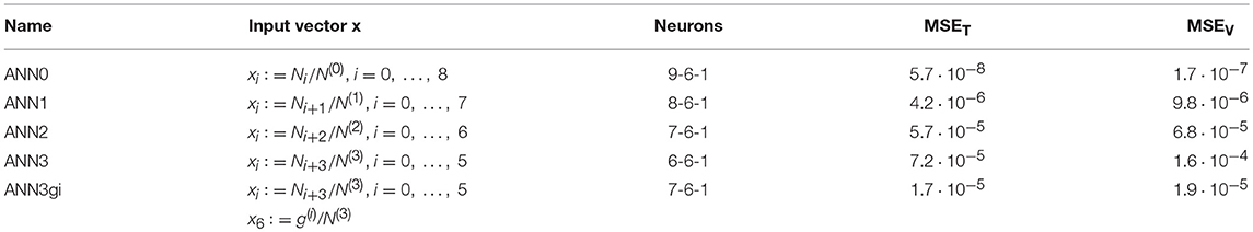
Table 2. ANN definitions and squared errors after training for varying degree of information about junctions with low coordination number.

FIGURE 7

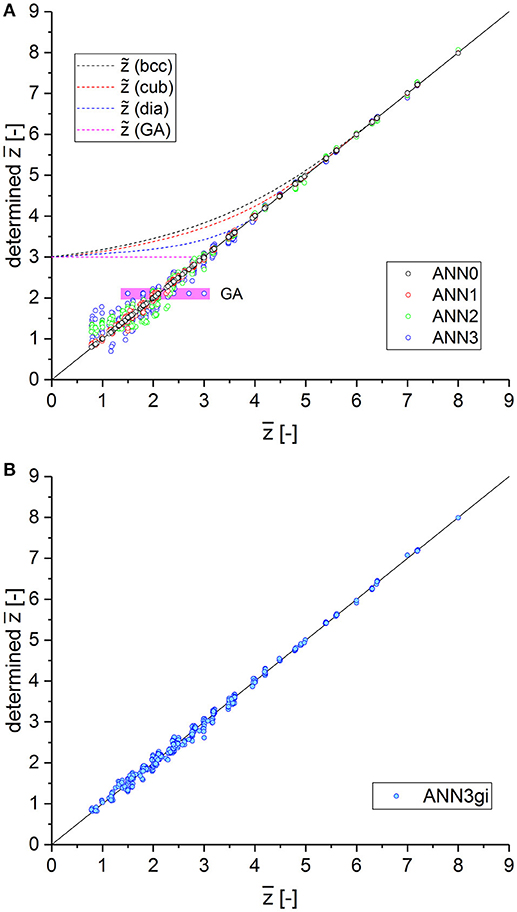
Figure 7. (A) Predicted ANN output vs. desired output for average coordination number $\overline{z}$ for continuous reduction of inputs with low coordination numbers from ANN0 (full information) to ANN3 (only junctions with coordination of 3 and higher). (B) ANN3gi incorporating an estimated scaled genus density of the inner structure as additional input. The performance of ANN3gi is better by a factor of 3 compared to ANN2.

For visualizing the performance of the ANN, an estimate of the average coordination number $\overline{z}$ is calculated by averaging all coordination numbers provided to the input for ANN3:

$\begin{array}{ll}\tilde{z}={\sum }_{z=3}^{8}z{N}_z/N^{\left(3\right)}.& (18)\end{array}$

It can be seen from Figure 7A that the machine-learning approach has the capability of interpreting the presented data in the context of the information of all structures provided during training. Knowing the big picture obviously helps to reconstruct missing information in the input data with reasonable accuracy. This can be understood by visualizing the statistical distribution of the local coordination numbers, which follow typical patterns according to the probability of cutting, as seen in Data Sheet 1, Supplementary Section 6.

Section Relationship Between Scaled Genus Density and Average Coordination Number leaves us with the question of whether the genus could provide additional linear independent information on the average coordination number. To investigate this, the input definition of the ANN can be enriched by adding an estimated scaled genus density using the accessible number of junctions in the structure, g/N⁽³⁾. Using such data, however, limits the generality of the approach to perfectly ordered structures. As soon as structures are randomized or cut in planes that do not meet planes of the unit cells, the genus is biased to lower values due to the cutting of originally closed curves. Thus, the incorporation of the genus requires an input definition that is insensitive to the boundary, similarly to the computation of $\overline{z}$ from junctions located inside the RVE. To this end, ligaments that touch the boundary are removed from the structure before calculating the genus of the inner graph, denoted as g⁽ⁱ⁾. The normalization by the number of detectable junctions inside the RVE boundaries, corrected to a structure of infinite size via the factor g_{V, ∞}/g_V,RVE (see Data Sheet 1, Supplementary Table 3), leads to an additional input g⁽ⁱ⁾/$N^{(3)}:=g_{RVE}^{(i)}$/$N^{(3)}·g_{V,\infty }/g_{V,RVE}$. This input definition works without any knowledge about the fully connected structure.

After training, this neural network, denoted as ANN3gi, performs better than ANN2 by a factor of 3, as can be seen from the mean squared errors in Table 2 and the predicted output data plotted in Figure 7B. This shows that the additional information on the scaled genus density, despite being a rough estimate of the mathematically correct value, particularly helps in reducing the uncertainty for $\overline{z}\le 3$.

Young's Modulus and Yield Strength

The master curve Equation (10) developed in section Young's Modulus brings the data generated for different structures very close to a single curve. For our data set, the accuracy compared to the master curve can be improved without limiting the generality of the approach. A second artificial neural network is trained, which corrects the macroscopic Young's modulus for each pattern relative to the prediction of the master curve Ẽ(ζ_tot), given by Equation (10). For reasons of consistency, we use the same input definition as used for ANN3 (see Table 2) but apply the following output definition:

$\begin{array}{ll}y:=E/E_{0,bcc}-Ẽ\left({\zeta }_{tot}\right).& (19)\end{array}$

After this artificial neural network, denoted as ANN3E, is trained, the mean squared training and validation error come to $MS{E}_T=1.21·10^{-3}$ and $MS{E}_V=1.03·10^{-3}$ respectively. An accuracy of ±0.01 for the output is reached, which is an improvement by a factor of 2 compared to the master curve. Only a few data points are located outside this limit. Trials including the estimate of the scaled genus density in the input definition, as used for ANN3gi, do not improve the result. This is possibly because this additional information is only relevant close to and beyond the percolation threshold, where the mechanical properties are anyway approaching zero.

In the same way as for the macroscopic Young's modulus, an artificial neural network ANN3sy is trained for correcting the macroscopic yield strength relative to the master curve, with the inputs as defined for ANN3 and the output definition being

$\begin{array}{ll}y:={\sigma }_y/{\sigma }_{y0,bcc}-{\tilde{\sigma }}_y\left({\zeta }_{tot}\right),& (20)\end{array}$

where ${\tilde{\sigma }}_y({\zeta }_{tot})\equiv Ẽ({\zeta }_{tot})$ is given by Equation (10). The yield strength shows a larger scatter in the numerical data and also larger deviations from the master curve, as seen in Figure 3. As a neural network interprets only the general relationship hidden in the data as whole, the scatter of the data is also reflected in the overall training error, which is double that of the Young's modulus. The resulting mean squared training and validation error are $MS{E}_T=5.22·10^{-4}$ and $MS{E}_V=4.99·10^{-4}$, respectively. The accuracy is improved by a factor of about 4 from the span of the training range from −0.03 to 0.06, with a remaining uncertainty of ±0.01. This uncertainty results from the sensitivity of the RVEs to local plastic yielding, which seems to be influenced more strongly by the realization of random cutting than the macroscopic Young's modulus.

An overview of the workflow developed in sections Macroscopic Mechanical Properties and 4 is given in Data Sheet 1, Supplementary Section 7. The Supplementary data files (Data Sheet 2) for training and validation of the ANNs are specified in Data Sheet 1, Supplementary Section 8; the ANNs are provided in Data Sheet 3 as Supplementary Python code including selected example problems as described in Data Sheet 1, Supplementary Section 9.

Validation and Application

Randomized Diamond Structures With Nodal Correction

Literature on NPG, studying the topological properties from artificially generated 3D structures and 3D FIB tomography, reports a large number of three-fold junctions and a smaller number of quadruple junctions (Mangipudi et al., 2016). A diamond structure, as suggested by Huber et al. (2014), can be tuned using the cut fraction to meet any ratio of three-fold and quadruple junctions. The randomization of the finite element beam model by an additional parameter A as a multiple of the unit cell size allows the prediction of realistic macroscopic properties, including Poisson's ratio (Huber et al., 2014; Roschning and Huber, 2016). A nodal corrected beam model can be applied, mimicking the effect of the nodal mass on the deformation behavior similar to a solid model (Jiao and Huber, 2017b).

To validate the approach developed in this work, we use such an extended model, which describes the elastic-plastic deformation behavior of NPG more realistically compared to the perfect 3D periodic structures without nodal masses employed in the previous section. To this end, additional structures with randomization values ranging from A = 0.1 to A = 0.3 and cut fractions ζ up to 0.4 are generated. Examples of RVEs of size N = 6 unit cells are given in Data Sheet 1, Supplementary Figure 3.

For all randomized structures, the chosen ligament radius is r/a = 0.118. The geometry and property parameters for the nodal corrected beam model are given in Data Sheet 1, Supplementary Section 1. In addition to the randomization, the major difference with perfectly ordered crystals is that distorted ligaments are now cut at the RVE boundaries. With increasing degree of randomization, the RVE also loses junctions that are shifted outside the RVE boundaries. This allows the approach to be tested for more general structures.

Topology

Figure 8A presents the results for the determined average coordination number $\overline{z}$ vs. the correct values. The solid curve indicates the exact solution. The ANN3 outputs (circles) agree for all three randomizations and are very close to the exact solution, with a slight trend for underestimation by −0.1. The results for the highest cut fraction ζ = 0.4 show the highest scatter toward low values by an average of −0.2 (on average 10% deviation) due to missing information on the statistics for coordination numbers $\overline{z}<3$. The comparison with the estimate $\tilde{z}$, on the other hand, shows that the ANN3 significantly improves the determination of the average coordination number for $\overline{z}<3.5$. The accuracy is further improved by including additional input g⁽ⁱ⁾/N⁽³⁾ (ANN3gi, cross symbols). The scatter is reduced compared to ANN3 and the outputs are very close to the correct values. Only for the lowest values of $\overline{z}$ does a slight underestimation along with some scatter occur.

FIGURE 8

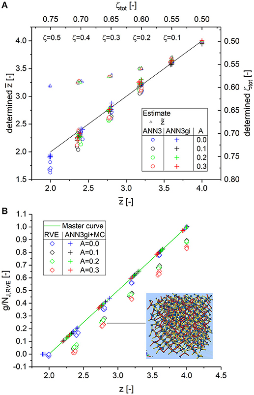
Figure 8. (A) Determination of average coordination number $\overline{z}$ for randomized diamond structures; outputs of ANN3 and ANN3gi and estimate $\tilde{z}$ for junctions with three or more branches; (B) scaled genus density and its dependence on the randomization of the RVE. The insert on the lower right exemplarily shows a structure for N = 4 and ζ = 0.3. For details, see Data Sheet 1, Supplementary Sections 1–3.

Based on the value of $\overline{z}$, the scaled genus density $g_V^{*}(\overline{z})=g/N_{J,RVE}$ is calculated from Equation (16), as seen in Figure 8B. After scaling the data for the perfectly ordered crystal (A = 0.0, blue diamonds) to infinite structure size by a factor of g_{V, ∞}/g_V,RVE = 1.314 (see Data Sheet 1, Supplementary Table 3), they fall nicely onto the master curve. As expected, the genus falls immediately below the master curve for the randomized structures, because about 50% of the distorted ligaments are now cut by the RVE boundary. A similar effect occurs in the analysis of tomographic data, where the boundary of the inspected volume is introduced artificially and does not exist as a real boundary in the larger sample. In this sense, the elevated values from the master curve Equation (16), calculated with the identified average coordination number from ANN3gi, reflect the scaled genus density of the infinite-size structure.

Macroscopic Young's Modulus and Yield Strength

According to the workflow depicted in Data Sheet 1, Supplementary Figure 10, the total cut fraction ζ_tot, calculated from $\overline{z}$ serves as key input for the prediction of the mechanical properties based on the master curves Equations (10, 13). Equation (11) determines the relevant part of the master curves. For z_dia/z_bcc = 0.5 and ζ = 0 to 0.5, we obtain the range for ζ_tot = 0.5 to 0.75 and the initial value E_{0, dia}/E_{0, bcc} = 0.239, as also seen in Data Sheet 1, Supplementary Table 1 for ζ_ini = 50%. The master curves are entered into Figure 9 as solid curves. The related cut fraction ζ, which is 0 for the fully connected diamond structure, is shown on the top axis of these plots. All numerical results are entered as solid symbols with the same color-coding as explained for Figure 9A for the different degrees of randomization.

FIGURE 9

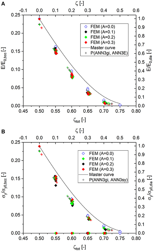
Figure 9. Simulation results and predicted macroscopic properties. Data points predicted by ANNs are denoted according to P(x, y). (A) Young's modulus; (B) yield strength. Zero values indicate simulations that were terminated before reaching a plastic strain of 0.2% due to bad convergence.

The plots for the Young's modulus and yield strength, as shown in Figures 9A,B, show no dependence on the degree of randomization. This supports the hypothesis that the scaling of mechanical properties, as formulated in Equation (6) for Young's modulus, holds. The values E/E_{0, bcc} and σ_y/σ_{y0, bcc}, as determined by the artificial neural networks ANN3E and ANN3sy, respectively, are added as cross symbols. Both ANNs are able to predict the displacement by about −0.02 relative to the master curve, thus resembling the position of the numerical data extremely well. Uncertainties in the determined total cut fraction appear as a scatter of the determined values along the displaced master curve. Only in the upper left corner of the plot are the values of E/E_{0, bcc} and σ_y/σ_{y0, bcc} displaced. It can be assumed that these specific data points are treated rather as outliers by the ANN during training, because fully connected diamond and Gibson–Ashby structures appear outside the overall trend in Figure 2B.

From Figure 9B, it can be seen that it is possible to predict the yield strength for RVEs that cannot be numerically solved due to convergence problems. This happens more often for increasing randomization and cut fraction, made visible by the frequency of green and red solid symbols with zero values. This nicely shows that the presented approach allows the prediction of macroscopic mechanical properties for structures that cannot be solved with computer simulations.

Poisson's Ratio

Figure 10A presents the results for the Poisson's ratio, which show different behavior for the three randomizations. While the data for A = 0.1 (black solid symbols) follow the master curve for all cut fractions, the data for A = 0.2 (green solid symbols) show a minimum value at ζ_tot = 65%, while values increase for higher cut fractions. This phenomenon, already observed for the perfect crystals (see Figure 4), is expected. However, for the RVE with maximum randomization of A = 0.3 (red solid symbols), the minimum value moves up to the starting point at zero cut fraction and all data show a very large scatter.

FIGURE 10

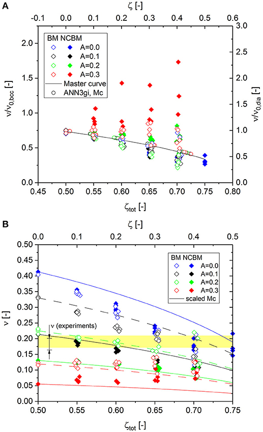
Figure 10. (A) Comparison of numerical results for elastic Poisson's ratio to the master curve for different degrees of randomization; (B) Absolute values of Poisson's ratio from FEM simulations plotted vs. total cut fraction. The range of experimental data is taken from Roschning and Huber (2016).

This deviation from the master curve motivates additional simulations for the same randomizations but without nodal correction. The results entered in Figure 10A as open symbols (beam model, BM) do not show such strong deviations. Up to A = 0.2, all data follow nicely on the master curve. However, for A = 0.3, a similar behavior can be observed as for the nodal-corrected RVE, with larger deviations for increasing cut fraction.

This seemingly odd behavior can be understood if it is considered that randomization has a strong effect on the elastic Poisson's ratio (Huber et al., 2014; Roschning and Huber, 2016; Jiao and Huber, 2017a) which rapidly decreases with increasing randomization. In addition, plotting the absolute values in Figure 10B shows that the nodal correction, combined with randomization, decreases the Poisson's ratio even further. This effect is not mentioned by (Jiao and Huber, 2017b), because in their study, nodal correction is only discussed in relation to the macroscopic stress-plastic strain response of the RVE.

Poisson's ratio is a critical parameter for the calibration of the randomization. Data from different sources display a range for NPG from ν = 0.165 to 0.2 (Roschning and Huber, 2016). This range, highlighted in yellow in Figure 10B, can now be analyzed with respect to the cut fraction as an additional degree of freedom. This limits the choice of realistic combinations of cut fraction and randomization, for which the deviation of the numerical data from the master curve is negligible. The sensitivity of Poisson's ratio is much stronger with respect to the randomization in comparison to the cut fraction. If the randomization is around A = 0.2, the data with nodal correction are even insensitive to the cut fraction. To calibrate the model by the experimental data, we can determine possible combinations (A, ζ) by moving from zero to maximum cut fraction along the yellow-shaded area. This again underlines the necessity of determining the average coordination number through a structural analysis. With the known average coordination number, the position on the x-axis (total cut fraction) is defined and Poisson's ratio can be used for calibrating the randomization parameter A.

Data From Macroscopic Compression Experiments

The determination of the effective solid fraction, which mechanically contributes to the ligament network of NPG, is the scope of the studies by Liu et al. (2016) and Liu and Jin (2017). The authors report a large range of samples with ligament sizes from 5 to 500 nm. The degree of connectivity was changed via the alloy composition prior to coarsening. Coarsening of sets of samples after dealloying for four different initial solid fractions gave a large set of samples, forming a valuable database. The measured macroscopic Young's modulus was used for determining the effective solid fraction. The major assumption is that only connected ligaments contribute to the mechanical stiffness, which is given by the Gibson–Ashby scaling relation Equation (1), rewritten as ${\phi }_{eff}={(E/E_s)}^{1/2}$. The difference between φ and φ_eff is attributed to dangling ligaments.

Determination of Cut Fraction

In this work, the mass of dangling ligaments corresponds to the fraction of cut ligaments according to

$\begin{array}{ll}\alpha ={\phi }_{\mathrm{\text{eff}}}/\phi =\left(1-\zeta \right).& (21)\end{array}$

In Equation (21), α is the fraction of load-bearing ligaments, as introduced by Liu et al. (2016) and Liu and Jin (2017). Consequently, ζ represents the fraction of cut ligaments as introduced in this work. For samples with lower solid fraction φ~0.26, the macroscopic Young's modulus takes very low values. As no percolation threshold is considered by Liu et al. (2016) and Liu and Jin (2017), the calculated effective solid fraction reaches values close to 0 and the cut fraction tends to 1. From the results of Soyarslan et al. (2018), we know that the network loses its connectivity at a solid fraction φ^P, which is why Equation (3) with φ^P = 0.159 and m = 2.56 should be used instead of Equation (1).

Combining the data from the studies by Liu et al. (2016) and Liu and Jin (2017) with Equation (3), plotted as suggested by Soyarslan et al. (2018), leads to Figure 11A. In this plot, symbols and colors correspond to those in Figure 4 of the study by Liu and Jin (2017). Soyarslan et al. (2018) selected the experimental data to include only as-prepared samples, ignoring samples where the ligament size was varied by annealing and using only the data from specimen with maximum connectivity (Jin et al., 2018). After including the data of the annealed specimen, a large scatter appears for each data set of constant solid fraction. This cannot be captured by Equation (3) as it uses the solid fraction φ as a sole parameter for the characterization of the structure. However, with the cut fraction as additional parameter, we have the degree of freedom that is needed for analyzing the data of Liu et al. (2016) and Liu and Jin (2017), depending on the fraction of dangling ligaments.

FIGURE 11

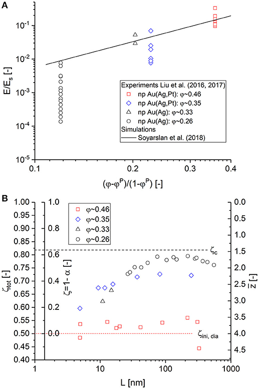
Figure 11. (A) Literature data for macroscopic Young's modulus E/E_s plotted vs. (φ−φ^P)/(1−φ^P) taken from experiments (Liu et al., 2016; Liu and Jin, 2017) and simulations (Soyarslan et al., 2018). (B) Cut fractions and average coordination numbers determined from the master curve in Equation (10), assuming diamond as reference structure.

From the statistical analysis of the skeletonized NPG structures presented by (Mangipudi et al., 2016), most junctions show a three-fold coordination, while a few percent with higher coordination numbers can also be detected. Assuming a Gibson–Ashby structure would limit the maximum coordination to 3, whereas a diamond structure can be adjusted to a similar statistical distribution, including some four-fold coordinated junctions, by cutting off ligaments.

Based on the assumption that a fully connected NPG material is described with a diamond structure, we can now analyze the data for macroscopic Young's modulus taken from Liu et al. (2016) and Liu and Jin (2017) and interpret the decay of the modulus for a given solid fraction in terms of cut fraction ζ. The values of ζ are determined by calibrating the modulus data to fit onto the maser curve for Equation (10) (see also Figure 2A). For the reference value, the average macroscopic Young's modulus of the data set with maximum solid fraction φ~0.46 is calibrated to match E_{0, dia}/E_{0, bcc} = 0.239. On the x-axis, ς_tot = 0.5 corresponds to z = 4 for diamond. It should be noted that the starting point can be set to any non-integer value in general when more precise information on the topology of the fully connected structure is available.

Relative to the value of E_{0, dia}/E_{0, bcc} = 0.239, the experimental data yield cut fractions, which are shown in Figure 11B for each data set at constant solid fraction depending on the ligament size, approaching the limits ζ_c = 0.822 and ${\overline{z}}_{min}\approx 1.5$ for the lowest modulus data. The determined cut fractions ζ qualitatively agree very well with the results for 1−α presented by Liu and Jin (2017). However, we determine different fractions of load-bearing ligaments. While Liu et al. report that < 10% of the ligaments remain for bearing load for φ~0.25, we have ≳40% load-bearing ligaments (< 60% cut fraction with respect to diamond). This is due to the percolation threshold that represents an upper limit for the cut fraction. On average, we determine the following values for the average coordination number $\overline{z}~2.5-3.0$ (φ~0.33−0.35) and $\overline{z}\lesssim 2$ (φ~0.26).

Determination of Yield Strength

Liu et al. inserted the effective solid fractions in the Gibson–Ashby scaling law for the yield strength given in Equation (2) to determine the yield strength of the solid fraction in each sample from the macroscopic yield strength (Liu et al., 2016). The findings of our work have two implications in this context: (i) the effective solid fraction is higher due to the percolation threshold, and (ii) the scaling of macroscopic Young's modulus and yield strength due to cutting of ligaments follow both the same relationship given by Equation (10), instead of Eqs. (1) and (2) with two different exponents 2 and 1.5, respectively. Whether this has a significant impact on the determined yield strength of the solid fraction can be investigated using the scaling laws, as applied by Liu et al. (2016) and Liu and Jin (2017): ${\sigma }_y/{\sigma }_{yS}=0.3{\phi }_{eff}^{3/2}$ and $E/E_S={\phi }_{eff}^2$. By solving E/E_S with respect to φ_eff and inserting the result in σ_y/σ_yS, the dependencies of the yield strength on the macroscopic Young's modulus are generated in the form ${\sigma }_y/{\sigma }_{yS}~{(E/E_S)}^{3/4}$.

According to section Young's Modulus, we have in fact σ_y/σ_yS ~(E/E_S) for a set of samples with constant solid fraction. This clearly shows that the yield strength would decrease faster with the exponent 1 instead of 0.75. A quantitative comparison is given in Figure 12A, where φ = 0.48 is assumed for the fully connected structure and φ_eff = αφ with α = 0.74 (Liu and Jin, 2017). As expected, the data confirm that the results do not depend on the chosen structure (diamond or Gibson–Ashby). Also, the linear fits in the log-log diagram confirm the exponents, as derived in the previous paragraph.

FIGURE 12

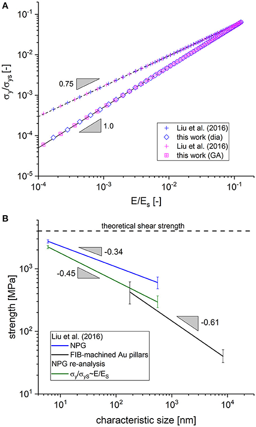
Figure 12. (A) Translation of macroscopic Young's modulus data to macroscopic yield strength according to Liu et al. (2016) and Equation (10). (B) Re-analysis of the data from Figure 8 of the study by Liu et al. (2016) with the data from (A).

We can furthermore conclude from Figure 12A that both curves converge for large values of macroscopic Young's modulus and yield strength (i.e., low cut fractions) while for lower values (or for higher cut fractions), the yield strength is overpredicted by Liu et al. (2016). By translating the quantitative behavior of the two curves into the diagram presented in Figure 12B, we obtain a very interesting result. The blue and the black curve both correspond to the fits of the data as entered in Figure 8 of the study by Liu et al. (2016), representing the yield strength as determined from NPG along with data collected by the authors from literature on FIB-machined Au pillars, respectively. It can be seen that an extrapolation of both curves for small characteristic sizes tend toward the theoretical shear strength. However, for larger characteristic size, the curves diverge.

The green curve results from translating the strength data of Liu et al. with the help of the data presented in Figure 12A to the correct scaling for increasing cut fraction, according to Equation (10). This lowers the strength values for larger characteristic sizes more than for small characteristic sizes and, within the experimental scatter, this closes the gap between the data from Au nanoligaments and FIB-machined Au pillars. The better agreement of the experimental results for larger ligament sizes is a strong support for the theoretical findings that (i) the macroscopic properties can be modeled as multiplicative decomposition of two terms, where one term depends only on the solid fraction and the second term depends on the cut fraction and (ii) the master curves for Young's modulus and yield strength show the same dependence on the cut fraction. Despite this promising outcome, the experimental validation presented here is only an indirect access whereas a direct validation would be much more desirable. To this end, artificial structures as generated in this work (for example see Data Sheet 1, Supplementary Figure 3) could be translated into specimen using additive manufacturing or 3D laser lithography technology. Elastic-plastic compression testing of specimen with varying initial structure and cut fraction would deliver the unchallengeable proof for the findings presented in this work.

Conclusions

This work addresses a number of fundamental questions regarding topological description and its incorporation in the structure-properties relationships of materials characterized by a highly porous three-dimensional structure. The findings are relevant for nanoporous metals and open-pore foams, morphologies of ordered block copolymers and polymer blends during spinodal decomposition, and architectured mechanical meta-materials consisting of struts or beams that undergo bending deformation.

Generalizing the highly efficient finite element beam models allows the generation of data for structures of different topologies, ranging from a highly coordinated bcc structure down to a Gibson–Ashby structure with a coordination number of three. What is common for all these structures is that they deform under bending of the ligaments. By random cutting of a fraction of ligaments in the RVE, selected structures were continuously modified with respect to their average coordination number from the value of the fully connected structure to the percolation-cluster transition. The macroscopic responses, such as Young's modulus, yield strength, and Poisson's ratio, were computed for each RVE. Together with the cut fraction, average coordination number, and statistical information about the local coordination within the structure, a database was created consisting of more than 100 different structures.

It is shown that the macroscopic Young's modulus, yield strength, and Poisson's ratio can be expressed in the form of a multiplicative decomposition, where the first term depends on the solid fraction and the second on the cut fraction. The dependence on the cut fraction can be represented by a master curve, covering a large range of structures beginning from highest coordination number of 8 of the bcc reference structure to 1.5, which is the average coordination number close to the percolation-cluster transition. Any average coordination number in between can be reached by the random cutting of a corresponding fraction of ligaments, as the average coordination number decreases linearly with increasing cut fraction.

As a striking result, all data for macroscopic Young's modulus and yield strength are covered by a single master curve, irrespective of whether perfectly ordered structures or more realistic randomized structures with nodal masses are considered. This leads to the important conclusion that the loss of strength due to pinching-off of ligaments is proportional to the decline in Young's modulus. Experimental support for this unexpected finding came from re-analyzing the data of Liu et al. (2016) and Liu and Jin (2017). The analysis shows that the gap between the strength data of Au nanoligaments and from FIB-machined micropillars can be neatly closed by incorporating this scaling behavior.

For the elastic Poisson's ratio, a second master curve was constructed that follows an elliptic-type shape with a maximum value for the fully connected structure and very low values with increasing cut fraction. In this case, the data show a divergence from the master curve for high cut fractions, which is probably caused by the beginning formation of clusters that do not follow the deformation pattern of the more connected parts of the structure. Beyond what is known for fully connected structures (Huber et al., 2014; Roschning and Huber, 2016), it turns out that the randomization needs to be calibrated for the correct value of the cut fraction (or average coordination number), because both structural parameters commonly define the elastic Poisson's ratio.

Based on the fingerprints of the different topologies, a scaling of the genus density could be identified that again combines all data in a single master curve with the average coordination number being the independent variable. The characteristic length that fulfils this condition normalizes the genus to the number of junctions of the fully connected structure. It is shown that linear relationships exist between all topological parameters under investigation, which are the total cut fraction, the average coordination number, and the scaled genus density. For proper measurement of each of these parameters, knowledge about the fully connected structure is required. This important detail significantly complicates the experimental measurement in each case.

An access to the solution to this central problem was found in machine learning. Feeding statistical information about the local coordination numbers of detectable junctions and, optionally, the estimated genus density, allows the determination of the average coordination number without knowledge of the fully connected structure. It could be shown that incorporating an estimate for the scaled genus density improves the accuracy by a factor of 3.5. Having determined the average coordination number, this parameter serves as a common key for the calculation of the cut fraction, the scaled genus density, and the mechanical properties with reference to a chosen fully connected structure.

Analyzing the data from the study by Liu and Jin (2017), the cut fraction for NPG samples with different solid fraction and degree of coarsening were determined, assuming a diamond structure as a fully connected reference. It turns out that the number of load-bearing ligaments with ≳40% is much larger compared to < 10% reported by Liu and Jin (2017), which is due to the incorporation of the percolation threshold. At the same time, the corresponding average coordination numbers falls slightly below 2, which corresponds to a scaled genus density of 0.

Author Contributions

NH conceptualized and designed the study. NH developed the Python scripts for object-oriented job creation and submission and organized the database. NH carried out the data-mining and machine-learning work. NH wrote and revised the manuscript.

Funding

Support from Deutsche Forschungsgemeinschaft (SFB 986 M³ project B4) is gratefully acknowledged.

Conflict of Interest Statement

The author declares that the research was conducted in the absence of any commercial or financial relationships that could be construed as a potential conflict of interest.

Acknowledgments

Jingsi Jiao is acknowledged for carrying out preliminary studies on RVEs with random cutting of ligaments. The author thanks Jörg Weissmüller (SFB 986 M³ project B2) for the intense discussions and valuable feedback throughout the development of this work. Particularly, section Relationship Between Scaled Genus Density and Average Coordination Number on the scaled genus density and its connection to the average coordination number would not exist without this highly inspiring interaction. Claudia Richert and Erica T. Lilleodden (SFB 986 M³ project B4) are acknowledged for discussions and careful reading of the manuscript, which have helped to strengthen the work.

Supplementary Material

The Supplementary Material for this article can be found online at: https://www.frontiersin.org/articles/10.3389/fmats.2018.00069/full#supplementary-material

References

Abaqus (2014). User's Manual Version 6.14-1. Providence, RI: Dassault Systémes Simulia Corp.

Ashby, M., and Bréchet, Y. (2003). Designing hybrid materials. Acta Mater. 51, 5801–5821. doi: 10.1016/S1359-6454(03)00441-5

CrossRef Full Text | Google Scholar

Ashby, M., Evans, A., Fleck, N., Gibson, L., Hutchinson, J., and Wadley, H. (2000). Metal Foams: A Design Guide. Oxford: Butterworth-Heinemann.

Google Scholar

Balk, T., Eberl, C., Sun, Y., Hemker, K., and Gianola, D. (2009). Tensile and compressive microspecimen testing of bulk nanoporous gold. J. Miner. 61, 26–31. doi: 10.1007/s11837-009-0176-6

CrossRef Full Text | Google Scholar

Biener, J., Hodge, A., and Hamza, A. (2007). Deformation Behavior of Nanoporous Metals. Micro and Nano Mechanical Testing of Materials and Devices. Livermore, CA: Lawrence Livermore National Laboratory.

Google Scholar

Biener, J., Hodge, A., Hayes, J., Volkert, C., Zepeda-Ruiz, L., Hamza, A., et al. (2006). Size effects on the mechanical behavior of nanoporous Au. Nano Lett. 6, 2379–2382. doi: 10.1021/nl061978i

PubMed Abstract | CrossRef Full Text | Google Scholar

Chupakhin, S., Kashaev, N., Klusemann, B., and Huber, N. (2017). Artificial neural network for correction of effects of plasticity in equibiaxial residual stress profiles measured by hole drilling. J. Strain Anal. Eng. Des. 52, 137–151. doi: 10.1177/0309324717696400

CrossRef Full Text | Google Scholar

Domb, C., and Sykes, M. (1961). Cluster size in random mixtures and percolation processes. Phys. Rev. 122, 77–78. doi: 10.1103/PhysRev.122.77

CrossRef Full Text | Google Scholar

Gibson, L., and Ashby, M. (1997). Cellular Solids: Structure and Properties, 2nd Edn. Cambridge: Cambridge University Press. doi: 10.1017/CBO9781139878326

CrossRef Full Text | Google Scholar

Gong, S., Li, Z., and Zhao, Y. Y. (2011). An extended Mori-Tanaka model for the elastic moduli of porous materials of finite size. Acta Materialia 59, 6820–6830. doi: 10.1016/j.actamat.2011.07.041

CrossRef Full Text | Google Scholar

Griffiths, E., Bargmann, S., and Reddy, B. (2017). Elastic behaviour at the nanoscale of innovative composites of nanoporous gold and polymer. Extrem. Mech. Lett. 17, 16–23. doi: 10.1016/j.eml.2017.09.006

CrossRef Full Text | Google Scholar

Haykin, S. (1998). Neural Networks. A comprehensive foundation. PTR Upper Saddle River, NJ: Prentice Hall.

PubMed Abstract | Google Scholar

Hu, K. (2017). Micromechanical and Three-Dimensional Microstructural Characterization of Nanoporous Gold–Epoxy Composites. Ph.D. Thesis, Hamburg University of Technology (TUHH).

Hu, K., Ziehmer, M., Wang, K., and Lilleodden, E. (2016). Nanoporous gold: 3D structural analyses of representative volumes and their implications on scaling relations of mechanical behaviour. Philos. Mag. 96, 3322–3335. doi: 10.1080/14786435.2016.1222087

CrossRef Full Text | Google Scholar

Huber, N., Nix, W., and Gao, H. (2002). Identification of elastic-plastic material parameters from pyramidal indentation of thin films. Proc. R. Soc. A 458, 1593–1620. doi: 10.1098/rspa.2001.0927

CrossRef Full Text | Google Scholar

Huber, N., Viswanath, R., Mameka, N., Markmann, J., and Weißmüller, J. (2014). Scaling laws of nanoporous metals under uniaxial compression. Acta Mater. 67, 252–265. doi: 10.1016/j.actamat.2013.12.003

CrossRef Full Text | Google Scholar

Husser, E., Soyarslan, S., and Bargmann, S. (2017). Size-affected dislocation activity in crystals: advanced surface and grain boundary conditions. Extrem. Mech. Lett. 13, 36–41. doi: 10.1016/j.eml.2017.01.007

CrossRef Full Text | Google Scholar

Ioannidis, M., and Lang, E. (1998). Microgeometry and topology of statistically homogeneous porous media. Trans. Ecol. Environ. 17, 223–230.

Google Scholar

Ioannidis, M. A., and Chatzis, I. (2000). On the geometry and topology of 3D stochastic porous media. J. Colloid Interface Sci. 229, 323–334. doi: 10.1006/jcis.2000.7055

PubMed Abstract | CrossRef Full Text | Google Scholar

Jang, D., Meza, L., Greer, F., and Greer, J. (2013). Fabrication and deformation of three-dimensional hollow ceramic nanostructures. Nat. Mater. 12, 893–898. doi: 10.1038/nmat3738

PubMed Abstract | CrossRef Full Text | Google Scholar

Jiao, J., and Huber, N. (2017a). Deformation mechanisms in nanoporous metals: effect of ligament shape and disorder. Comput. Mater. Sci. 127, 194–203. doi: 10.1016/j.commatsci.2016.10.035

CrossRef Full Text | Google Scholar

Jiao, J., and Huber, N. (2017b). Effect of nodal mass on macroscopic mechanical properties of nanoporous metals. Int. J. Mech. Sci. 134, 234–243. doi: 10.1016/j.ijmecsci.2017.10.011

CrossRef Full Text | Google Scholar

Jin, H.-J., Weissmüller, J., and Farkas, D. (2018). Mechanical response of nanoporous metals: a story of size, surface stress, and severed struts. MRS Bull. 43, 35–42. doi: 10.1557/mrs.2017.302

CrossRef Full Text | Google Scholar

Jinnai, H., Kajihara, T., Watashiba, H., Nishikawa, Y., and Spontak, R. (2001). Interfacial and topological measurements of bicontinuous polymer morphologies. Phys. Rev. E Stat. Nonlin. Soft Matter Phys. 64:010803. doi: 10.1103/PhysRevE.64.010803

PubMed Abstract | CrossRef Full Text | Google Scholar

Kováčik, J. (1999). Correlation between Young's modulus and porosity in porous materials. J. Mater. Sci. Lett. 18, 1007–1010. doi: 10.1023/A:1006669914946

CrossRef Full Text | Google Scholar

Kwon, Y., Thornton, K., and Voorhees, P. (2010). Morphology and topology in coarsening of domains via non-conserved and conserved dynamics. Philos. Mag. 90, 317–335. doi: 10.1080/14786430903260701

CrossRef Full Text | Google Scholar

Lilleodden, E., and Voorhees, P. (2018). On the topological, morphological, and microstructural characterization of nanoporous metals. MRS Bull. 43, 20–26. doi: 10.1557/mrs.2017.303

CrossRef Full Text | Google Scholar

Liu, L.-Z., and Jin, H.-J. (2017). Scaling equation for the elastic modulus of nanoporous gold with “fixed” network connectivity. Appl. Phys. Lett. 11:211902. doi: 10.1063/1.4984108

CrossRef Full Text | Google Scholar

Liu, L.-Z., Ye, X.-L., and Jin, H.-J. (2016). Interpreting anomalous low-strength and low-stiffness of nanoporous gold: quantification of network connectivity. Acta Mater. 118, 77–87. doi: 10.1016/j.actamat.2016.07.033

CrossRef Full Text | Google Scholar

Liu, R., and Antoniou, A. (2013). A relationship between the geometrical structure of a nanoporous metal foam and its modulus. Acta Mater. 61, 2390–2402. doi: 10.1016/j.actamat.2013.01.011

CrossRef Full Text | Google Scholar

Lührs, L., Zandersons, B., Huber, N., and Weissmüller, J. (2017). Plastic poisson's ratio of nanoporous metals: a macroscopic. Nano Lett. 17, 6258–6266. doi: 10.1021/acs.nanolett.7b02950

PubMed Abstract | CrossRef Full Text | Google Scholar

Mameka, N., Wang, K., Markmann, J., Lilleodden, E., and Weissmüller, J. (2015). Nanoporous gold—testing macro-scale samples to probe small-scale mechanical behavior. Mater. Res. Lett. 4, 27–36. doi: 10.1080/21663831.2015.1094679

CrossRef Full Text | Google Scholar

Mangipudi, K., Epler, E., and Volkert, C. (2016). Topology-dependent scaling laws for the stiffness and strength of nanoporous gold. Acta Mater. 119, 115–122. doi: 10.1016/j.actamat.2016.08.012

CrossRef Full Text | Google Scholar

Nachtrab, S. (2011). Percolation and Elasticity of Networks—From Cellular Structures to Fibre Bundles. Erlangen-Nürnberg: Friedrich-Alexander-Universität Erlangen-Nürnberg (FAU). urn:nbn:de:bvb:29-opus-30736

Google Scholar

Nachtrab, S., Kapfer, S., Arns, C., Madadi, M., and Mecke, K. (2011). Morphology and linear-elastic moduli of random network solids. Adv. Mater. 23, 2633–2637. doi: 10.1002/adma.201004094

PubMed Abstract | CrossRef Full Text | Google Scholar

Nachtrab, S., Kapfer, S., Rietzel, D., Drummer, D., Madadi, M., Arns, C., et al. (2012). Tuning elasticity of open-cell solid foams and bone scaffolds via randomized vertex connectivity. Adv. Eng. Mater. 14, 120–124. doi: 10.1002/adem.201100145

CrossRef Full Text | Google Scholar

Phani, K., and Niyogi, S. (1987). Young's modulus of porous brittle solids. J. Mater. Sci. 22, 257–263. doi: 10.1007/BF01160581

CrossRef Full Text | Google Scholar

Pia, G., and Delogu, F. (2015). Nanoporous Au: statistical analysis of morphological features and evaluation of their influence on the elastic deformation behavior by phenomenological modeling. Acta Mater. 85, 250–260. doi: 10.1016/j.actamat.2014.11.040

CrossRef Full Text | Google Scholar

Richert, C., and Huber, N. (2018). Skeletonization, geometrical analysis and finite element modeling of nanoporous gold based on 3D tomography data. Metals 8:282. doi: 10.3390/met8040282

CrossRef Full Text | Google Scholar

Richeson, D. S. (2008). Euler's Gem—The Polyhedron Formula and the Birth of Topology. Princeton, NJ: Princeton University Press.

Google Scholar

Roberts, A., and Garboczi, E. (2002). Elastic properties of model random three-dimensional open-cell solids. J. Mech. Phys. Solids 50, 33–55. doi: 10.1016/S0022-5096(01)00056-4

CrossRef Full Text | Google Scholar

Roschning, B., and Huber, N. (2016). Scaling laws of nanoporous gold under uniaxial compression: effects of structural disorder on the solid fraction, elastic Poisson's ratio, Young's modulus and yield strength. J. Mech. Phys. Solids 92, 55–71. doi: 10.1016/j.jmps.2016.02.018

CrossRef Full Text | Google Scholar

Sahimi, M. (1994). Applications of Percolation Theory. London: Taylor and Francis.

Google Scholar

Scheiner, S., Pivonka, P., and Hellmich, C. (2016). Poromicromechanics reveals that physiological bone strains induce osteocyte-stimulating lacunar pressure. Biomech. Model. Mechanobiol. 15, 9–28. doi: 10.1007/s10237-015-0704-y

PubMed Abstract | CrossRef Full Text | Google Scholar

Soyarslan, S., Bargmann, S., Pradas, M., and Weissmüller, J. (2018). 3D stochastic bicontinuous microstructures: generation, topology and elasticity. Acta Mater. 149, 326–340. doi: 10.1016/j.actamat.2018.01.005

CrossRef Full Text | Google Scholar

Sun, X.-Y., Xu, G.-K., Li, X., Feng, X.-Q., and Gao, H. (2013). Mechanical properties and scaling laws of nanoporous gold. J. Appl. Phys. 113:023505. doi: 10.1063/1.4774246

CrossRef Full Text | Google Scholar

Sykes, M., and Essam, J. (1964). Critical percolation probabilities by series methods. Phys. Rev. 133, A310–A315. doi: 10.1103/PhysRev.133.A310

CrossRef Full Text | Google Scholar

Tyulyukovskiy, E., and Huber, N. (2006). Identification of viscoplastic material parameters from spherical indentation data: part I. Neural Netw. J. Mater. Res. 21, 664–676. doi: 10.1557/jmr.2006.0076

CrossRef Full Text | Google Scholar

Tyulyukovskiy, E., and Huber, N. (2007). Neural networks for tip correction of spherical indentation curves from bulk metals and thin metal films. J. Mech. Phys. Solids 55, 391–418. doi: 10.1016/j.jmps.2006.07.003

CrossRef Full Text | Google Scholar

Weissmüller, J., Newman, R., Jin, H.-J., Hodge, A., and Kysar, J. (2009). Nanoporous metals by alloy corrosion: formation and mechanical properties. MRS Bull. 34, 577–586. doi: 10.1557/mrs2009.157

CrossRef Full Text | Google Scholar

Willumeit, R., Feyerabend, F., and Huber, N. (2013). Magnesium degradation as determined by artificial neural networks. Acta Biomater. 9, 8722–8729. doi: 10.1016/j.actbio.2013.02.042

PubMed Abstract | CrossRef Full Text | Google Scholar

Yagawa, G., and Okuda, H. (1996). Neural networks in computational mechanics. Arch. Comput. Methods Eng. 3, 435–512. doi: 10.1007/BF02818935

CrossRef Full Text | Google Scholar

Zaoui, A. (2002). Continuum micromechanics: survey. J. Eng. Mech. 128, 808–816. doi: 10.1061/(ASCE)0733-9399(2002)128:8(808)

CrossRef Full Text | Google Scholar

Zheng, X., Lee, H., Weisgraber, T., Shusteff, M., DeOtte, J., Duoss, K., et al. (2014). Ultralight, ultrastiff mechanical metamaterials. Science 344, 1373–1377. doi: 10.1126/science.1252291

PubMed Abstract | CrossRef Full Text | Google Scholar

Ziehmer, M., Hu, K., Wang, K., and Lilleodden, E. (2016). A principle curvatures analysis of the isothermal evolution of nanoporous gold: quantifying the characteristic length-scales. Acta Mater. 120, 24–31. doi: 10.1016/j.actamat.2016.08.028

CrossRef Full Text | Google Scholar

Ziman, J. M. (1968). The localization of electrons in ordered and disordered systems I. Percolation of classical particles. J. Phys. C (Proc. Phys. Soc.) 1, 1532–1538.

Google Scholar