A General Modeling Approach for Shock Absorbers: 2 DoF MR Damper Case Study

1 Introduction

A dynamic mathematical model for an automotive shock absorber must accurately simulate its behavior and accommodate nonlinearities (e.g., friction, hysteresis, and inertia) over a frequency range with a maximum value lower than 30 Hz in the automotive field. The characteristics of the Force-Velocity (FV) and Force-Displacement (FD) diagrams of an automotive shock absorber are crucial. Table 1 summarize the acronym definitions. Many modeling methods currently exist. The ideal method needs to be generic and allows the adjustment of a model based on a visual analysis of the characteristic diagrams because these provide the information for the design of the suspension. A Passive (p) Shock Absorber has a damping capacity defined by its mechanical design that varies with the displacement and oscillation frequency. Its FV and FD characteristic diagrams are constant, and it may be designed for comfort or surface grip (or a balance of both). Semi-Active (SA) shock absorbers have a capacity defined by their mechanical design and by an external signal that causes one of its mechanical properties to vary. When there is no external signal, their state is P. Their FV and FD diagrams can vary. The three most commonly used commercial technologies are p, Magneto-Rheological (MR), and Electro-Hydraulic (EH); these are compared in Table 2.

TABLE 1

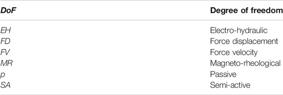
TABLE 1. Acronym definitions.

TABLE 2

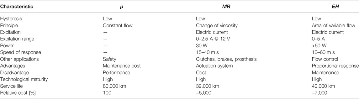
TABLE 2. Comparison of the different shock absorber technologies.

Some models have been developed with parameters that have no physical meaning, such as 1) p, Duym (1997), 2) MR, Choi et al. (2001) and Savaresi et al. (2005b), and 3) EH, Codeca et al. (2008). The models that have parameters with physical meaning, such as the phenomenological models, are also classified as 1) p, Duym (2000) and Carrera-Akutain et al. (2006), 2) MR, Wang and Kamath (2006) and Choi et al. (2001), and 3) EH, Heo et al. (2003). Examples of models whose parameters are linked to the characteristic diagrams are 1) p, Basso (1998) and Calvo et al. (2009) and 2) MR, Guo et al. (2006) and Ma et al. (2007). The latter are of primary interest because the parameters can predict the efficiency of the shock absorber during a vehicle maneuver. Table 3 summarizes the variables definition.

TABLE 3

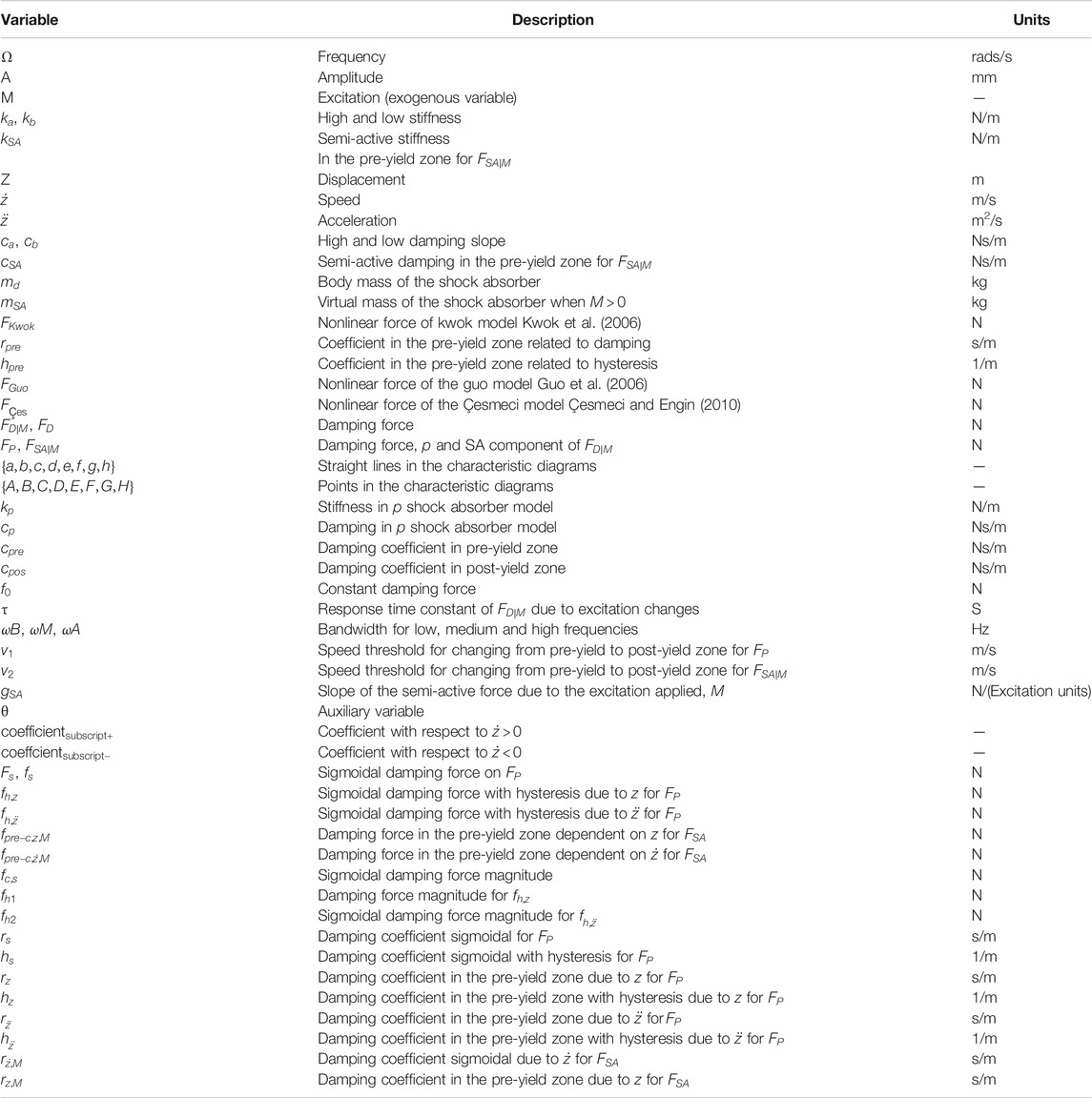
TABLE 3. Variables definition.

Because the FV diagram resembles a sigmoid function, three models have successfully used trigonometric functions (hyperbolic tangent and arc tangent) to model hysteresis. Kwok et al. (2006) proposed using a function that includes hysteresis based on the sign of the displacement:

$F_{\text{Kwok}}=\text{tanh}\left[\underset{\text{dampening}}{\underbrace{r_{\text{pre}}\dot{z}}}+\underset{\text{hysteresis}}{\underbrace{h_{\text{pre}}sign\left(z\right)}}\right](1)$

Guo et al. (2006) introduced a function that depends on both the sign and the displacement magnitude:

$F_{Guo}=\text{tanh}\left(\underset{\text{dampening}}{\underbrace{r_{pre}\dot{z}}}+\underset{\text{hystresis}}{\underbrace{h_{pre}z}}\right)(2)$

Çesmeci and Engin (2010) combined the force and hysteresis using a sigmoid function and the acceleration sign:

$F_{\text{Çes}}={\text{tan}}^{-1}\left[\underset{\text{dampening}}{\underbrace{r_{pre}\dot{z}}}+\underset{\text{hysteresis}}{\underbrace{h_{pre}sign\left(\ddot{z}\right)}}\right](3)$

The results are satisfactory in terms of the FV diagrams for constant frequencies, amplitudes, and excitations, but are nevertheless limited in precision in terms of dynamics. Sims et al. (2004) proposed a method of high precision results, but the model was not generalized and required specific tests. Ma et al. (2007) proposed the modification of p shock absorber models by multiplying the force by a current-dependent force. Boggs (2009) developed a nonlinear model that included hysteresis using a delay of force with a first-order filter; it did not include the friction associated with the stiffness of the mechanical design. All the proposals presented above are computationally costly. Table 4 compares these models.

TABLE 4

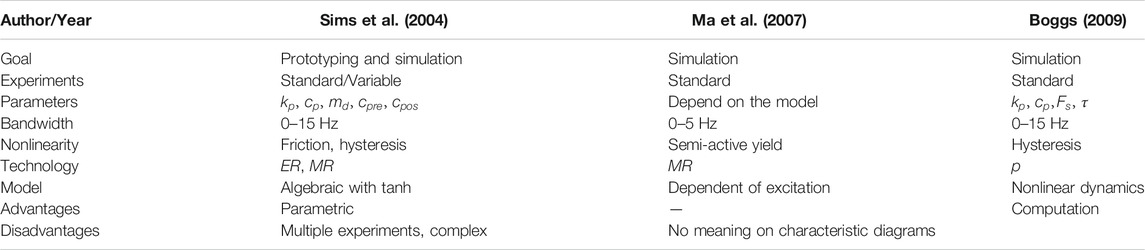
TABLE 4. Models comparison.

A generic model design method based on characteristic diagrams to obtain a model that can be identified and simulated with a generic tools is proposed, Lozoya-Santos et al. (2015). The methodology proposes the decomposition of the measured force in two components: p and SA force components, Figure 1.

FIGURE 1

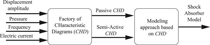
FIGURE 1. General block diagram of the CHD-based approach for shock absorbers modeling.

This paper deals particularly with the suitability of this method to understand and model a damper using its characteristic diagrams when it has one damping control input. The specimen to be used in this work has two control inputs, Golinelli and Spaggiari (2017): electric current and the pressure in the accumulator. In this context, the work focuses on the application of the method to analyze the effect of more than one control input on the damping force and in the characteristic diagrams, and a further method extension to include such effects. Other phenomenal aspects such as cavitation due to a fault of the damper and leaks of oil or pressure from the damper are out of scope. Section 2 presents the fundamentals of the method, and Section 3 describes the method. The proposal is demonstrated using a case study in Section 4 where all steps are implemented in detail. Finally, the research project is concluded in Section 5.

2 Fundamentals

The total force of a semi-passive shock absorber can be expressed with two terms, Dixon (2008):

$F_{D|M}=F_P+F_{SA|M}(4)$

where F_D|M is the total force given a certain excitation M, F_p is the term related to mechanical phenomena, and F_SA|M is the term related to the excitation M.

When F_D = F_P, the shock absorber is p.

2.1 Characteristic Diagrams

The characteristic diagrams show the kinematic performance when the excitation is zero F_D|M = 0. When force $F_{SA|M\ne 0}=F_{D|M\ne 0}-F_P$ is evaluated, the characteristic diagrams are denoted as SA and show the controllable dampening variation due to an exogenous variable, ideally independent of the kinematics.

The exogenous variable affects the SA characteristic diagrams depending on the technology. For MR and ER, the variable modifies the fluid and therefore the dynamic of the stiffness and dampening coefficients in the FD and FV diagrams. For EH, the FV diagram will vary proportionally to the exogenous variable, and the dynamics of the FD diagram are independent. The FD, FV and force-acceleration (FA) characteristic diagrams shown in Figure 2 can be represented by eight lines $\left\{a,\dots ,h\right\}$ and eight points $\left\{A,\dots ,H\right\}$; each x line is followed by a point X. These points represent events caused by kinematics and/or the exogenous variable and are common in the three diagrams; we refer to them as characteristic points. The direction of the curves is clockwise in the FD and FV diagrams and counterclockwise in the FA diagram.

FIGURE 2

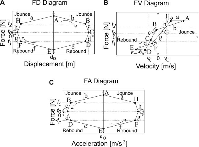
FIGURE 2. Characteristic diagrams.

There are three types of points in the characteristic diagrams. Yield point is the point at which the slope of the line decreases. In the FV and p diagrams, this point is related to the actuation of valves with a larger orifice at a limit speed. In the FV and SA diagrams, it is related to the change in behavior of the fluid (viscous to viscoplastic). Point of return is the point at which the speed changes direction and the slope of the line changes sign. It is present in all FV diagrams. Restoring point is the point at which the slope of the line increases with the same sign. In the FV and p diagrams, it occurs when the valve system deactivates the larger orifice valves and increases the damping. In the FV and SA diagrams, the chains formed by the magnetic phenomenon in the MR/ER fluid are restored, causing a sudden increase in the viscosity of the fluid. The yield and restoring points are related to the two main damping coefficients: high and low coefficient, Rakheja and Sankar (1985), Warner (1996), Hong et al. (2002), and Savaresi and Spelta (2007). A ratio higher than 5:1 for the high/low coefficient in extension and compression can be used for a symmetric shock absorber, and a ratio higher than 2:1 in compression can be used for an asymmetric shock absorber. Any changes in these specifications in the FV diagram will be reflected in the FD and FA diagrams. Table 5 shows the quadrants where the characteristic points are found based on the FV diagram.

TABLE 5

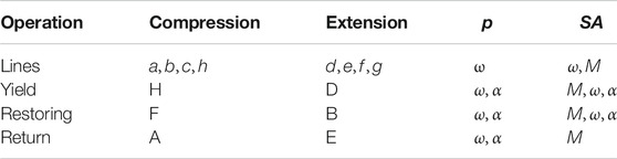
TABLE 5. Characteristic points in the FV diagram.

The analysis of the characteristic diagrams will be performed in three frequency ranges relevant to the automotive field: low frequency (ωB) [0.5–3] Hz, medium frequency (ωM) [3–7] Hz and high frequency (ωA) [7–15] Hz, Warner (1996). The slopes of the lines and coordinates of the characteristic points change according to: 1) oscillation frequency, ω; 2) oscillation amplitude (α) of the displacement of the piston in the p diagrams (p), and 3) the exogenous variable M.

In p diagrams, FD diagrams (Figure 2A) show a low stiffness, represented by slope $k_b$ in all lines for $\omega B$. The slope of the stiffness increases, $k_a$ in lines $c,d,g,h$, and in lines $a,b,e,f$ it tends to be zero for frequencies in the $\left[\omega M-\omega A\right]$ range. The slopes always have the same sign as the speed $sign\left(\dot{z}\right)$, Table 6 (the variables that most affect the slopes are shown). In the SA diagrams and FD diagrams, the lines have a $k_{SA}$ slope that is similar across the speed range in $\omega B$. This slope is the same for lines $c,d,g,h$ and tends to be zero in lines $a,b,e,f$ for $\omega M$ and $\omega A$. The slopes are always positive, Table 6.

TABLE 6

TABLE 6. FD line diagram for the p and SA cases.

The p diagrams and FV diagrams (Figure 2B) reveal high damping, represented by slope $c_a$ in all lines for $\omega B$. With damping, the slope $c_a$, does not change in lines $c,d,g,h$, and in lines $a,b,e,f$ tending to be a low damping, the slope $c_b$ tends to be less for frequencies in the $\left[\omega M-\omega A\right]$ range. In the $\omega A$$c_b\to 0$ range, Table 7, the slopes are always positive and affected by ω. In the SA diagrams, with regard to the FV diagrams, a large damping $c_{SA}$ of the lines is similar across the speed range in $\omega B$. This slope is the same for lines $c,d,g,h$, and tends to be zero in lines $a,b,e,f$ for $\omega M$ and $\omega A$. The slopes are always positive and are mainly affected by ω and M at low frequencies and by M only in $\omega M$ and $\omega A$, Table 7.

TABLE 7

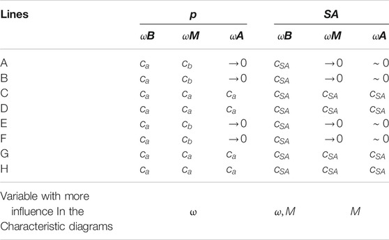
TABLE 7. FV line diagram for the p and SA cases.

In the p diagrams, FA diagrams (Figure 2C), the slope is almost zero in lines $a,b,e,f$ and infinite for $c,d,g,h$ in $\omega B$. Acceleration does not affect the force. The slope md appears in all the lines $\left[\omega M-\omega A\right]$. The frequency greatly affects the force due to its quadratic effect on acceleration. The slopes are always positive, Table 8. In the SA diagram, the slopes in $\omega B$ and $\omega M$ are the same as in $\omega B$ in the p diagrams. The acceleration has no effect on the SA force. At high frequencies, $\omega A$, it is possible to observe a positive slope, $m_{SA}$ for yield lines $a,b,e,f$. The acceleration does not affect the SA force significantly, Table 8.

TABLE 8

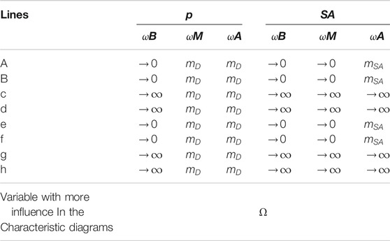
TABLE 8. FA line diagram for the p and SA cases.

A model is presented for each frequency range; for $\omega B$ is:

$F_{D|M}=\underset{F_P}{\underbrace{k_{b}sign\left(\dot{z}\right)z+c_a\dot{z}+m_{d}s\ddot{z}}}+\underset{F_{SA|M}}{\underbrace{M\left[k_{SA}z+c_{SA}\dot{z}\right]}}(5)$

For frequencies $\omega M$ and $\omega A$, the force components $F_P$ and $F_{SA|M}$ of the proposed model in Eq. 4 are as follows:

$F_P=\{\begin{array}{l}{k}_{a}sign\left(\dot{z}\right)z+c_a\dot{z}+m_d\ddot{z}\dot{z}<v_1\\ F_p\left(v_1\right)+c_b\dot{z}+m_d\ddot{z}\dot{z}>v_1\end{array}(6)$

$F_{SA|M}=\{\begin{array}{l}M\left(k_{SA}z+c_{SA}\dot{z}\right)\dot{z}<v_2\\ M\left[g_{SA}sign\left(\dot{z}\right)\right]+m_{SA}\ddot{z}\dot{z}>v_2\end{array}(7)$

The three equations are similar to that presented by Joarder (2003); however, the characteristic points are dynamic and have a function of frequency ω, amplitude α, and excitation M, Table 5. To propose a generic dynamic model, we classified the characteristic diagrams FD, FV, and FA according to the frequency range and the combination of characteristic points. The proposed classification has seven patterns: 1) Type 0 for $\omega B$, 2) Types (1, 2, 3, 4) for $\omega M$, and 3) Types (5, 6) for $\omega A$.

Type-0. In diagrams p, points A, B, and H are equal in compression and points D, E, and F are the same between them. If the shock absorber is asymmetric, the slopes of lines d and g are the same and different from those of lines c and h, which have the same slope, Figure 3. If the shock absorber is symmetric, then E = -A, D = -H and F = -B.

FIGURE 3

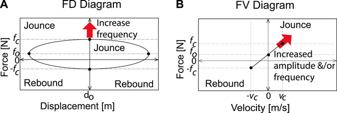
FIGURE 3. Characteristic diagrams at $\omega B$, Type-0.

The FD diagram shows a constant compressibility, k_b, with perfect ovals, Figure 3A. The FV diagram is a line with high damping $c_a$, Figure 3B. Slopes D, C, G, and H are equal. Lines A, B, E, and F have zero length. It is highly unusual for these to show hysteresis in the FV diagram. The effect of acceleration is negligible, Figure 4A. The frequency and amplitude of the displacement increases the magnitude of the characteristic points. In the SA diagrams, the frequency and amplitude of the displacement as well as the exogenous variable increase the characteristic points. The latter is the most significant in the ordinates of the points.

FIGURE 4

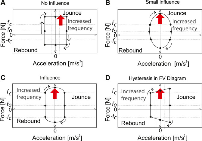
FIGURE 4. Types of FA characteristic diagrams.

Type-1. In the p case, this is the ideal type for an automotive shock absorber, Figure 5. The yield, restoring, and return points are all present. The high slopes of lines c and h, and of d and g are equal, just as the slopes of lines a and b in compression, and f and e in extension are the same. The yield points H and D, and restoring points B and F are the same between them in the compression quadrants, as well as the two that correspond to the extension quadrant. There is no hysteresis. The effect of acceleration is negligible, Figures 4A and 4B. This type does not exist in SA systems.

FIGURE 5

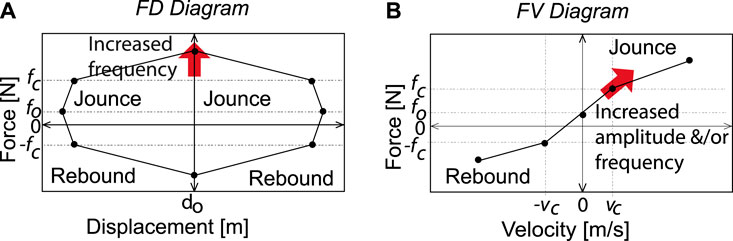
FIGURE 5. Characteristic diagrams at $\omega M$, Type-1.

Type-2. These are the typical diagrams of an automotive shock absorber, Figure 6. The difference with respect to Type-1 is that the abscissa and ordinate of the yield point H are greater compared to the restore point B. This causes hysteresis at high speed due to the viscosity of the fluid. The effect of acceleration may not be significant, Figure 4B. This diagram type is typical of SA diagrams, although it is regularly idealized at high speeds and represented as Type-1. The characteristics of the MR/ER fluid define the dynamic of the yield and restoring points.

FIGURE 6

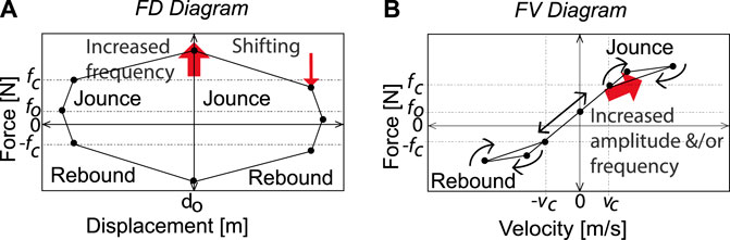
FIGURE 6. Characteristic diagrams at $\omega M$, Type-2.

Type-3. This type is also observed in automotive applications, Figure 7. The abscissa and ordinate of point B are smaller than those of point H, resulting in line b being longer than line a. The abscissa of B is much smaller than that of H; in particular, point B is closer to zero in the horizontal speed axis and further from zero in the horizontal displacement axis. This behavior causes hysteresis at low speed due to the compressibility of the fluid. When there is symmetry, point F = -H, and point F = -B. The effect of acceleration is negligible Figure 4A. These phenomena are typical in SA diagrams, but at high frequencies the viscosity of the MR/ER fluid does not have as fast a response as the oscillation frequency, causing a difference in the yield and restore points and generating hysteresis.

FIGURE 7

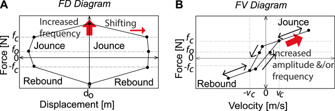
FIGURE 7. Characteristic diagrams at $\omega M$, Type-3.

Type-4. This type is atypical of p diagrams. It is the expected response of force $F_{SA|M=cte}$ in a shock absorber, Figure 8. The force is independent over almost the entire speed range, except in the vicinity of $\dot{z}=0$. If the force in this vicinity tended to be zero, then force SA would be ideal. The slopes of a, b, f, and e are zero due to the independence of speed at medium and high magnitudes. The yield points are H and D = -H, and the restore points are B and F = -B for symmetric cases. The points of return A and E = -A are equal, and their ordinate is equal in magnitude to yield points H and F = -H. The ordinate of the yield points is proportional to the magnitude of the exogenous variable. The slopes of lines c, d, g, and h may be sensitive to speed and to the exogenous variable and can increase as either variable increases. The change of the abscissa is very small, from five to 1. There is no hysteresis in the FV diagram, and the effect of acceleration is not significant, Figures 4A or Figure 4B.

FIGURE 8

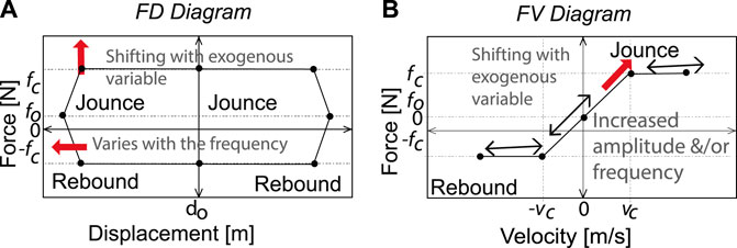
FIGURE 8. Characteristic diagrams at $\omega M$, Type-4.

Type-5. In p diagrams, this type may appear in extreme operating conditions, Figure 9. It is a mix of Type-2 and Type-3, and there is hysteresis due to the compressibility and viscosity phenomena of the fluid. The effect of acceleration may be significant, Figure 4C. This type is atypical of SA diagrams unless the shock absorber is ER/MR or if there is hysteresis in the response of the proportional valves.

FIGURE 9

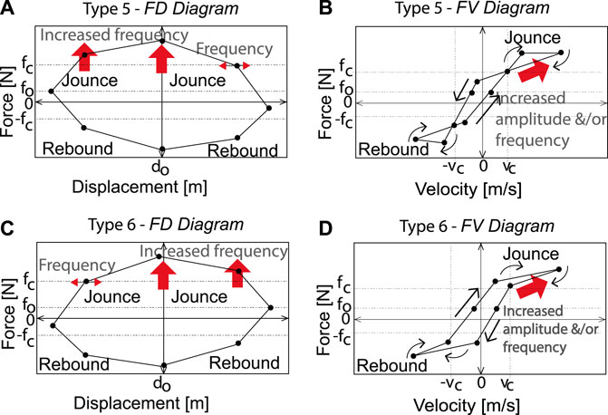
FIGURE 9. Characteristic diagrams at $\omega A$, Type-5 and Type-6.

Type-6. This type is very unusual for an automotive shock absorber, Figures 9C and 9D. The ordinates (force) of restore points B and F increase, and the ordinates of yield points D and H decrease. Due to the high frequency (speed), the yield and restore points occur faster, namely, Types-2 and Types-3 are inverted because the mechanical components are forced and do not recover their designed operating condition. The effect of acceleration is highly significant, Figure 4D. This type is atypical of SA diagrams.

2.2 Generic Model Definition

The proposed generic model of the shock absorber includes two terms.

$F_D=F_{P+,-}+F_{SA+,-}(8)$

where $F_{P+,-}$ is the component of the damper force $F_D$ associated with the passive part, that is, when the input (exogenous input, for example current) is zero, $F_{SA+,-}$ is the component of the damper force $F_D$ when the input (exogenous input, for example current) is different from zero, that is to say, it is the semi-active component (SA) of the shock absorber. The subscripts +, − can represent the mechanical exerted force of the shock absorber when the velocity is positive, +, or negative, −. In model identification, the parameter identification method gets the values of the model parameters using two sets of the data. Each set corresponds to positive and negative velocity, respectively. This model definition applies if the FV characteristic diagram presents non-linear and non-isotropic behavior (e.g., the behavior is not similar when the shock absorber is in a state of tension rather than in compression), Figure 10B.

FIGURE 10

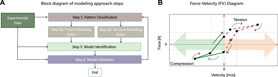
FIGURE 10. Basic methodology (A) The description of the methodology step by step, (B) A characteristic diagram Force-Velocity pointing the tension and compression shapes of the force, the arrows divide the diagram in positive and negative velocities. Sometimes it will be necessary to have identified model parameter values depending on the sign of the velocity of the piston.

F_P term definition. The first term is F_P, which models the behavior when an exogenous variable is not applied;

$F_P=f_0+c_p\dot{z}+k_{p}z+m_D\ddot{z}+f_s+f_{h,z}+f_{h,\ddot{z}}(9)$

where:

$\begin{array}{l}{f}_s=f_{c,s}\left(\frac{r_s\dot{z}+h_{s}z}{1+\left|r_s\dot{z}+h_{s}z\right|}\right)\\ f_{h,z}=f_{h_1}\left(\frac{r_z\dot{z}+h_{z}sign\left(z\right)}{1+\left|r_z\dot{z}+h_{z}sign\left(z\right)\right|}\right)\\ f_{h,\ddot{z}}=f_{h_2}\left(\frac{r_{\ddot{z}}\dot{z}+h_{\ddot{z}}sign\left(\ddot{z}\right)}{1+\left|r_{\ddot{z}}\dot{z}+h_{\ddot{z}}sign\left(\ddot{z}\right)\right|}\right)\end{array}$

Equation 9 is the F_P term of the force of the SA shock absorber. Coefficient f₀ is an initial compensation force; c_p is the viscous damping coefficient that describes the speed dependent force and is related to as c_b. The internal stiffness coefficient, k_p, represents the displacement dependent force and is related to k_b. The virtual mass m_D describes the acceleration dependent force, f_s = F_Guo, which is the damping force that represents the sigmoidal behavior. Finally, terms $f_{h,z}=F_{Kwok}$ and $f_{h,\ddot{z}}=F_{\text{Çes}}$ model the hysteresis effect at $\omega B$ and $\omega A$. To ensure a computationally efficient system, it uses a squash function, Yonaba et al. (2010), $f\left(\theta \right)=\theta /\left(1+\left|\theta \right|\right)$ where θ is the function argument that defines the sigmoidal form, instead of the frequently used hyperbolic tangent.

F_SA term definition. The second term is the F_SA, which models the force when the exogenous variable acts on the damping, Eq. 8. Because the shock absorber SA may have asymmetric behavior in the FV diagram, the coefficients of the model are different for positive and negative speeds.

$F_{SA}=M{g}_{SA}\left[f_{pre-c,\dot{z},M}+f_{pre-c,z}\right](10)$

where:

$\begin{array}{l}{f}_{pre-c,\dot{z},M}=\left(\frac{r_{\dot{z},M}\dot{z}M}{1+\left|r_{\dot{z},M}\dot{z}M\right|}\right)\\ f_{pre-c,z}=\left(\frac{r_{z,M}z}{1+\left|r_{z,M}z\right|}\right)\end{array}$

Equation 10 is the $F_{SA}$ term, where $g_{SA}$ is the gain in force per each M unit, the $f_{pre-c,\dot{z},M}$ term simulates force SA at low speeds at which damping depends on the speed and excitation, and $f_{pre-c,M}$ simulates the stiffness effect on force SA.

3 Modeling Approach

This methodology is divided in four steps, Figure 10A.

Step 1: Pattern classification.

The first step of the methodology is to classify the pattern of the characteristic diagram that was generated experimentally from the shock absorber. This classification allows the definition of the specific model equation from a set of options. The classification uses the type patterns defined and built for the p and SA forces: {Type-0, … , Type-6 } according to Section 2.1.

Step 2a: Modeling Rules for the $F_P$ term.

A set of rules defines the model for the $F_P$ term, Table 9. If the shock absorber is passive, the method considers only these rules. The base Eq. 9 suits the shock absorber performance in terms. To perform this step, it must have computed all the characteristic diagrams in the bandwidths of interest and for the displacement, velocity and acceleration. The logic to follow is: if the type of diagram in the $\omega B$, $\omega M$ and $\omega A$ bandwidths corresponds to a set of column values, then the $F_P$ term of the $F_D$ model adds the term indicated in the column Function to the term $F_P=f_0+c_p\dot{z}+k_{p}z+m_D\ddot{z}$. Then, the $F_P$ term takes the name indicated in the Model column of Table 9.

Step 2b: Modeling Rules for the $F_{SA}$ term.

TABLE 9

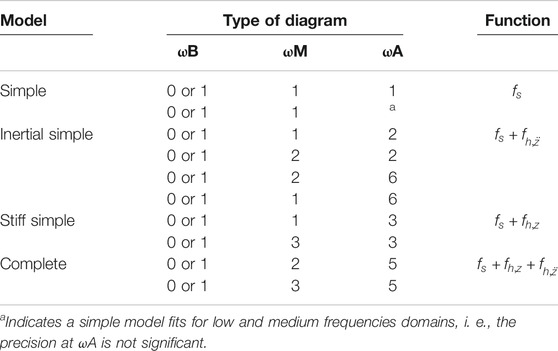
TABLE 9. Rules for modeling the p diagrams. ωA

Similarly, a set of rules defines the model for the $F_{SA}$ term, Table 10. The base Eq. 10 models the semi-active force in a characteristic diagram of a shock absorber when it acts the exogenous input with a signal M. The logic to follow is: if the type of diagram in the $\omega B$, $\omega M$ and $\omega A$ bandwidths corresponds to a set of column values, then the $F_{SA}$ term of the $F_D$ model becomes the term indicated in the column Function to the model $F_D=F_P$. Then, the $F_{SA}$ term takes the name indicated in the Model column of Table 10.

TABLE 10

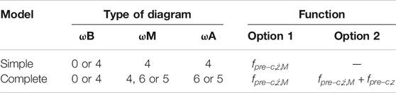
TABLE 10. Rules for modeling the SA characteristic diagrams.

Symmetry of the damping force in the characteristic diagrams. If the shock absorber is symmetric, damping force equals in shape and magnitude in tension and compression zones (positive and negative forces), the method proposes the following formulation:

$F_D=\underset{\text{passive force}}{\underbrace{f_0+c_p\dot{z}+k_{p}z+m_D\ddot{z}+{\text{function}}_{\text{PAS}}}}+\underset{\text{Semi}-\text{active force}}{\underbrace{M{g}_{SA}\left({\text{function}}_{SA}\right)}}(11)$

If the shock absorber is asymmetric, the method proposes to consider a generic model as in Eq. 12.

$F_D=f_0+\{\begin{array}{l}\underset{\text{passive force}}{\underbrace{c_{p+}\dot{z}+k_{p+}z+m_{D+}\ddot{z}+{\text{function}}_{PAS+}}}+\underset{\text{semi}-\text{active force}}{\underbrace{M{g}_{SA+}\left[{\text{function}}_{SA+}\right]}}\dot{z}>0\\ \underset{\text{passive force}}{\underbrace{c_{p-}\dot{z}+k_{p-}z+m_{D-}\ddot{z}+{\text{function}}_{PAS-}}}+\underset{\text{semi}-\text{active force}}{\underbrace{M{g}_{SA-}\left[{\text{function}}_{SA-}\right]}}\dot{z}\le 0\end{array}(12)$

where the subscript signs indicate if the speed is positive (+) or negative (-).

Step 3: Model identification

The identification process of the model uses the trust-region reflective optimization algorithm, Coleman and Li (1996). The nonlinear least-squares optimization method with the sum of squared errors objective function and the bounded solution space of parameters to be identified applies this algorithm. The main non-linearities that relate the input data to the output data are saturation and hysteresis. When the calculations from the identification data result in indefinite derivatives (very noisy data or with unpredictable discontinuities), use direct search methods, Wright (1996). These methods can be useful when experimental data from different tests are used as a single sequence of serial data to carry out the identification because there will be discontinuities developed at the end of each test data set joined sequentially.

Step 4: Model validation

To validate the results, the Error-to-Signal Ratio (ESR) index is proposed, which is the quotient of the variance of the estimation error and the variance of the experimental force, Savaresi et al. (2005a). Testing and identification data are different. An $ESR\sim 0$ indicates that the model is perfect; while an $ESR\sim 1$ indicates a trivial model that estimates an average value. If the result is not satisfactory, we suggest using patterns {Type-0, … , Type-6 } for the classification. If the identified model does not fill the precision needs, the methodology suggests reviewing the characteristic diagrams to reclassify the pattern types and repeat the model definition process and validation. .

Figure 11 specifies the proposed methodology. The identification of the mathematical modeling of four commercial shock absorbers (p, continuous MR, On/Off MR, and a continuous EH technology) validates this method, Lozoya-Santos et al. (2015). The models produced less than 5% of modeling error, evidenced in a set of qualitative plots and quantitative indexes.

FIGURE 11

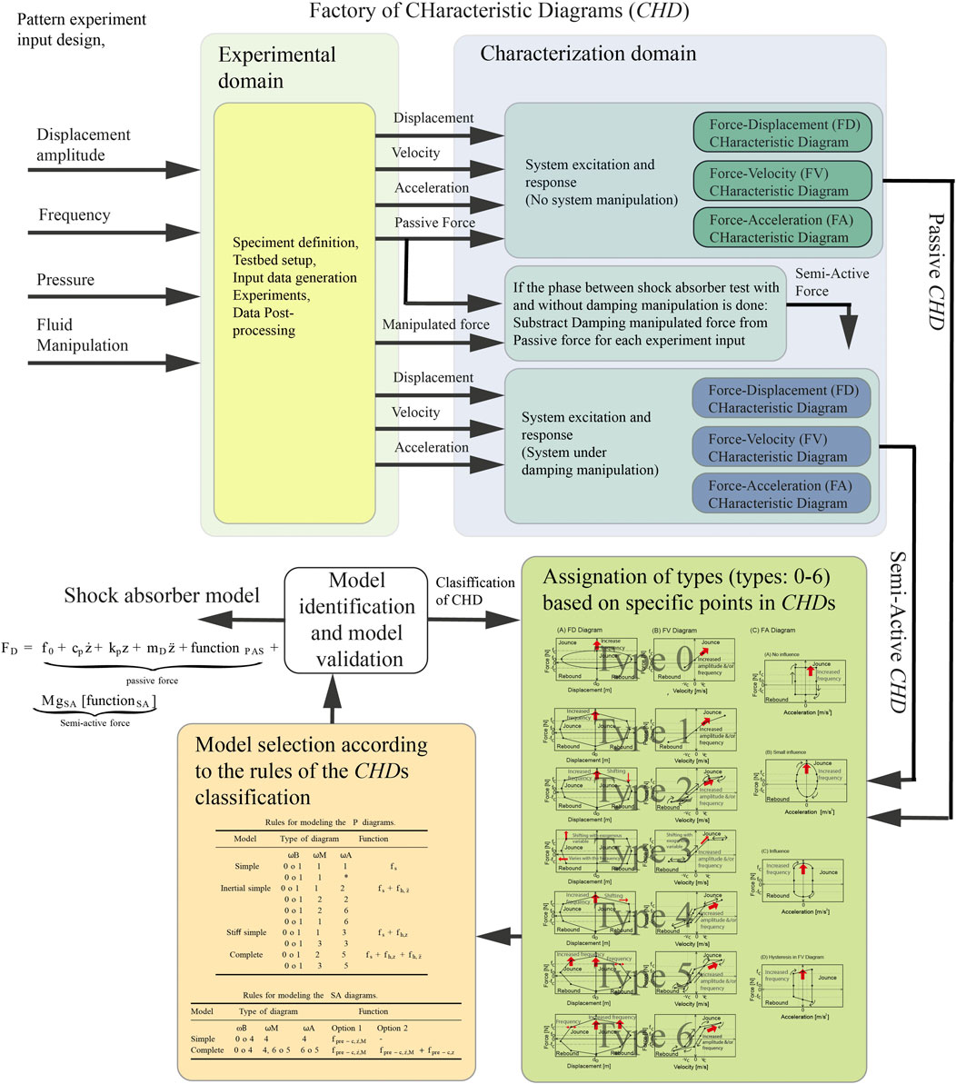
FIGURE 11. Block diagram describing the generation of characteristic diagrams from experimental data. For details on the Model identification and model validation (white) block output see the equations in Section 3. The tables inside the block Model selection according to the rules of CHDs classification are Tables 9 and 10. Regarding the block Assignation of types (types: 0–6) based on specific points in CHDs see Section 2 and Figures 3–9.

4 Case Study

4.1 2-Degree-of-Freedom (2DoF) MR Damper

A MR damper prototype has a novel architecture that differs from the existing ones by the presence of an internal counter-rod placed at the bottom of the damper, Golinelli and Spaggiari (2015), Figure 12. It uses a bottom-rod fixed to the end plug and coupled with the piston head. The bottom-rod has the same diameter of the upper-rod so that there is no volume variation. During piston movement, the bottom-rod is moving the chamber obtained into the piston head. The chamber is also directly connected to the canal through the upper-rod to bring out the wire of the coil. In such a manner, this configuration avoids the over-pressure or depression phenomenon within the chamber. Two coils were adopted. The longer axial length of the piston head allows maximizing the concatenated magnetic flux. The pressure system is composed of a stepper motor that converts the motion from rotary to translatory by a screw and nut mechanism. This system controls a slider that insists on the volume of MR fluid. Lowering the volume of fluid causes an increase of the internal pressure. The magnetic flux array (incoherent multiple coils) decreases of the overall inductance of the circuit that allows, compared to others, less response time of the same device.

FIGURE 12

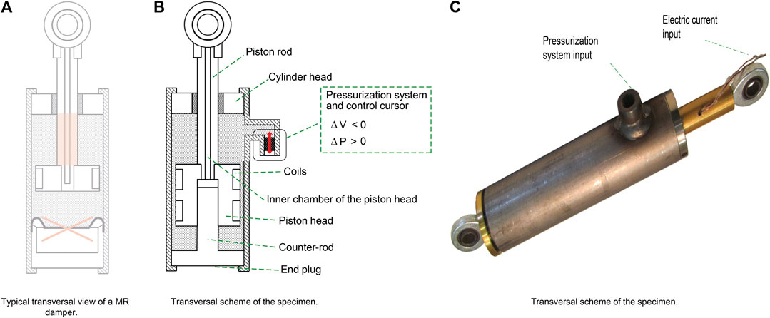
FIGURE 12. Architecture of the 2DOFMR Damper specimen and assembly.

The system works without the volume compensator and presents a precise internal pressure control. The architecture includes no protruding elements, a thermal compensation system, and cavitation prevention. For full details on the design and explanation of the functioning of this specimen, see Golinelli and Spaggiari (2017). The MR damper assembly uses commercial components: a hydraulic cylinder, its cylinder head, and two ball joint ends. The piston rod, the piston head, and the bottom rod are manufactured custom parts. The prototype, Figure 12C, shows the electric current as well as the pressure inputs. Golinelli and Spaggiari (2015). The technical specifications of the 2DoF-MR damper is listed in Table 11.

TABLE 11

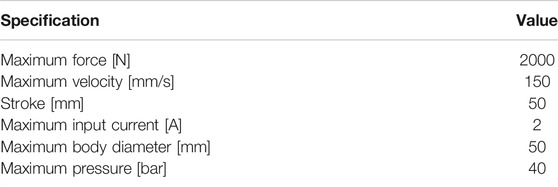
TABLE 11. 2DoF MR Damper technical specifications.

This device shows cavitation phenomena when no pressure is applied. On the other hand, when pressure is applied, it shows a similar behavior expected from a MR damper, no matter the applied level of electric current, Golinelli and Spaggiari (2017). The inclusion of cavitation in mathematical models of (p or SA) shock absorbers it is not a trivial task.

The Design of Experiments (DoE) methodology for this specimen and the experimental data was presented in Golinelli and Spaggiari (2017). The damper was tested under sinusoidal displacements. The variables involved are amplitude A and frequency f of the sinusoidal input, current I and a pressure level p. The chosen amplitude level was 5 mm. Each test lasted for 20 cycles with a sampling rate of 512 Hz. DoE was selected, a summary of the used variables and their values are reported in Table 12. For the testbed and details of the sensor and instrumentation system, please see Golinelli and Spaggiari (2017).

TABLE 12

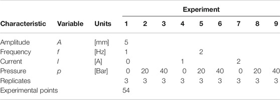
TABLE 12. DoE specification of the used experimental data in this modeling approach. The maximum velocity value ($V_{max}=2Af$ ) is 31.41 mm/s.

We would like to add that the sinusoidal test pattern and constant current permits the identification of precise models for the motion dynamics. These data patterns allow describing the non-linearities of the damper force with a persistent frequency at different manipulations, Tudon-Martinez et al. (2019) addressing the hysteresis phenomenon due to the friction and inertia. It is of interest to use this signal since it allows evaluating the vehicle vertical dynamics of the suspension at different frequencies, including the resonance frequencies of the chassis (around 1–2 Hz) and unsprung mass (around 8–9 Hz) in typical cars of class 1 Lozoya-Santos et al. (2012b) and Poussot-Vassal (2008). Moreover, it has been evidenced that this pattern performs good model parameter identification since a cross validation process with other richer displacement dynamics experiments has shown high precision in damping force estimation, Lozoya-Santos et al. (2012a). Regarding the dynamic response of the damping force due to a change in the electric current, typically the MR/ER fluid transient responses are between 20 and 30 m s before the reach of the steady state, Lozoya-Santos et al. (2012a). So, a first order model with these dynamics is typically added in the semi-active damper model electric current input/voltage to include the transient responses Lozoya-Santos et al. (2012b) and Savaresi et al. (2005b). The use of the sinusoidal test has been validated in a previous work where we compare the input motion patterns, and this signal was well suited to model damper nonlinearities, compared with white noise content signals. This paper’s scope regarding stroke displacement frequency is focused on a body comfort evaluation bandwidth.

4.2 Results

This subsection shows, step by step, the method application for the modeling of the described specimen in Section 4.

Step 1. Generation of the characteristic diagrams and its pattern classification.

The first step consists of the plotting of the characteristic diagrams FD and FV for all the experiments in Table 12. Figures 13 and 14 show the plots and a similar behavior due to the effect of the pressure and the electric current increments. The cavitation is present when the displacement changes its direction and crosses the zero of the vertical axis, i.e., negative displacement, positive force, and positive displacement and negative force. In such a moment, the cavitation appears as a change of slope of the damping force vs. the displacement. This phenomenon is present repetitively in each cycle for each test, amplitude, and electric current when internal pressure is 0 bar, Figures 13A–C.

FIGURE 13

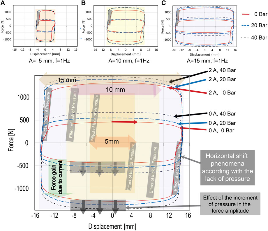
FIGURE 13. FD Characteristic diagrams for a 2 Degrees of Freedom MR shock absorber for the three cases of electric current (0, 1 and 2 A) and pressure (0, 20 and 40 bar). The first upper row shows the three FD diagrams for the different amplitudes. The second row shows the FD diagram, where it is emphasized the effects of pressure and electric current on the damping force, and how it changes according to the displacement amplitude.

FIGURE 14

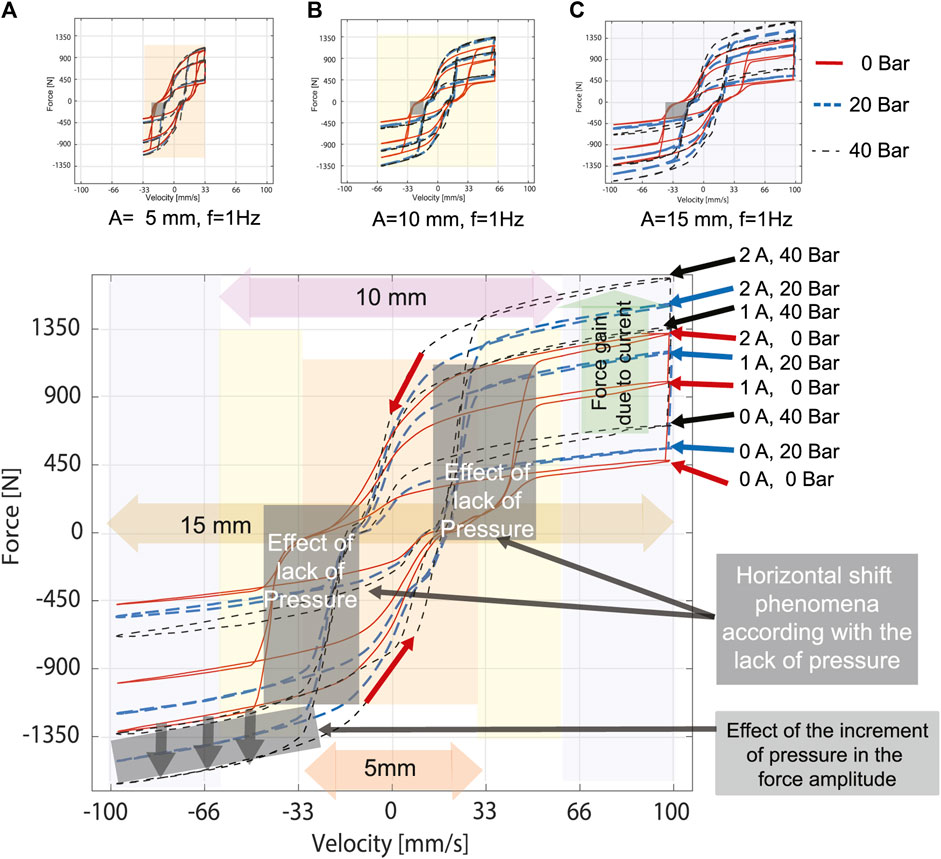
FIGURE 14. FV Characteristic diagrams for a 2 Degrees of Freedom MR shock absorber for the three cases of electric current (0, 1 and 2 A) and pressure (0, 20 and 40 bar). The first upper row shows the three FV diagrams for the different amplitudes. The second row shows a FV diagram, where it is emphasized the effects of pressure and electric current on the damping force, and how it changes according to the velocity amplitude.

When the internal pressure changes to 20 and 40 bar respectively, the cavitation and the dynamics in the vicinity of zero phenomena decrease considerably. Regarding to the presence of pressure, it supplies a damping force increment in a quasi-linear ratio, Figure 13 second row, approximately a 5N/bar. The effect of the increment of electric current, it is similar to well-known MR dampers in literature. The increment of electric current generates an approximated change with a ratio 500N/A.

In the FV characteristic diagram, the effect of the lack of pressure (0 bar) increases the complexity of the hysteresis phenomena. When the force tends to be zero from the yield zone, a monotonic decrement on the slope force-velocity before the zero force, and a monotonic increment of the slope after the zero appears, until the force yielding point. These dynamics modifies the typical hysteretical behavior of these devices. A final remark, the FV diagram qualitatively shows a left shift between positive and negative force over the horizontal axis, Figures 14A–C. Regarding to the internal pressure increment, a quasi linear force gain for each unit of pressure can be seen, Figure 14, since from 0 to 20 bar, the force gain is different than from 20 to 40 bar.

The total damping force, f_D, shows the above-mentioned dynamics in the vicinity of zero in the transient response, Figure 15A. It can be seen how the force increases for a change in the electric current magnitude. The semi-active forces due to the electric currents, $f_{SA|1A}=f_{D|1A}-f_{D|0A}$, and $f_{SA|2A}=f_{D|2A}-f_{D|0A}$ also reflects the effect of the pressure around zero force crossings, Figure 15B.

FIGURE 15

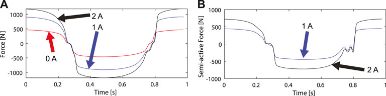
FIGURE 15. The transient behavior of the damping forces in the specimen for a 5 mm experiment, 20 bar input pressure and the three values of electric current: (A) damping force $f_D$ for 0A, 1A and 2A, (B) semi-active force due only to the electric current for 1A and 2A (computed by subtraction) $f_{D|1A,20Bar}-f_{D|0A,20Bar}$, and $f_{D|2A,20Bar}-f_{D|0A,20Bar}$.

The p and SA characteristic diagrams FD, FV, and FA display some of the specific patterns to do the classification. The p diagrams present similar characteristics to the type 3 with the influence of the acceleration in the damping force because of the shape of the FA plot, Figures 16A–C. Regarding the semi-active damping force characteristic diagrams, the shapes classifies as a type five, regardless of the added dynamics for the pressure input in the vicinity of zero force.

FIGURE 16

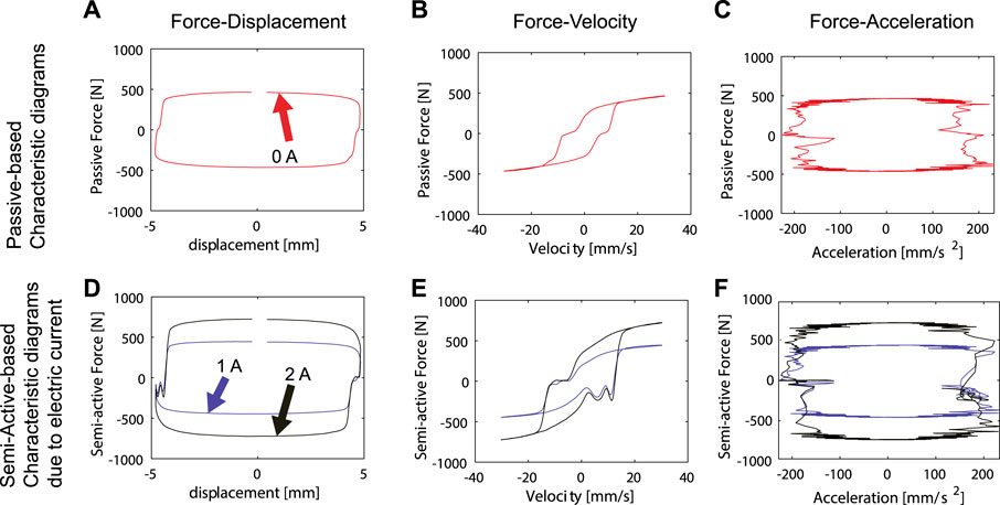
FIGURE 16. Characteristic diagrams according to the proposed method. The FD, FV and FA characteristics diagrams for p (first row) and SA (second row) forces agree with specified types in classification schemes.

The characteristic diagrams of the pressure vs. the force when the electric current is constant, Figure 17, compares the force dynamics when pressure is not present and when it increments in a constant ratio. It shows the FD and FV characteristics diagrams for the semi-active force generated from 0 to 20 Bars $\left(f_{D|20bars}-f_{D|0bars}\right)$, Figure 17(first row) and the semi-active force generated from 20 to 40 Bars $\left(f_{D|40bars}-f_{D|20bars}\right)$, Figure 17(second row). The analyzed experimental data set is the 5 mm amplitude data set for all the electric currents and pressures. For the subtraction $f_{D|20bars}-f_{D|0bars}$, a peak of semi-active damping force (which shows a linear effect on the magnitude of the electric current) appears on both characteristic diagrams, Figure 17 (first row). However, when the analyzed semi-active force corresponds to the damping force generated due to the change from 20 to 40 bars, it seems that the peak is not present in the diagram. There is no cavitation, Figure 17 (second row). So, this method of analysis can be used to detect such a condition of the shock-absorber.

FIGURE 17

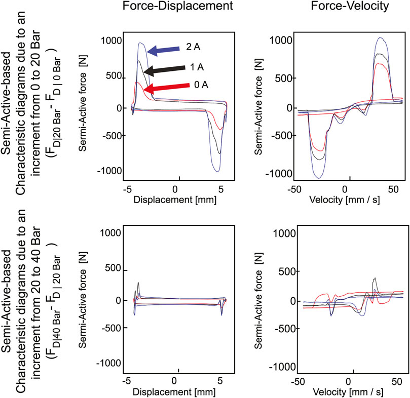
FIGURE 17. Characteristic diagrams of the semi-active force generated by the constant increments of the pressure according to the proposed method.

Steps 2a and 2b: Modeling Rules for the $F_P$ and $F_{SA}$ terms.

According to Table 9 for the p diagrams and Table 10 for the SA diagrams, the proposed classification, Table 13, sets the modeling approach focused on two model types: a) a model one based on the stiffness simple model for the p force and the complete model for the SA force, b) a complete-complete model in both forces.

Step 3: Model identification

TABLE 13

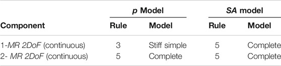
TABLE 13. Classification of characteristic diagrams and proposed models. It only takes into account one frequency, since the analyzed test is a 1 Hz signal.

The model identification process used the experimental set with 20 bar, since when the pressure is present, the complexity of the dynamics diminishes to that of a typical MR damper. All the amplitudes and electric current values were included. All the possible models were identified, Table 14. The lowest ESRs correspond to the model Stiffness Simple - Simple and for the model Complete-Complete. This result agrees with the model selection according to the presented methodology.

TABLE 14

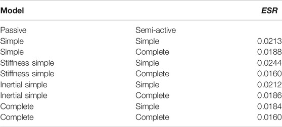
TABLE 14. Model estimation performances using ESR index.

The identified parameters for the Complete-Complete MR damper model is shown in Table 15.

Step 4: Model validation

TABLE 15

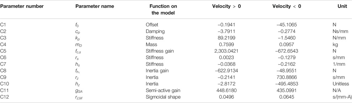
TABLE 15. Identified model parameters for the Complete-Complete approach.

The characteristic diagrams, Figures 18A–C, the forces comparison, Figure 18D, the relation electric current vs. force, Figure 18E and the transient response, Figure 18F, qualitatively show the proposed model matches with the MR damper dynamics.

FIGURE 18

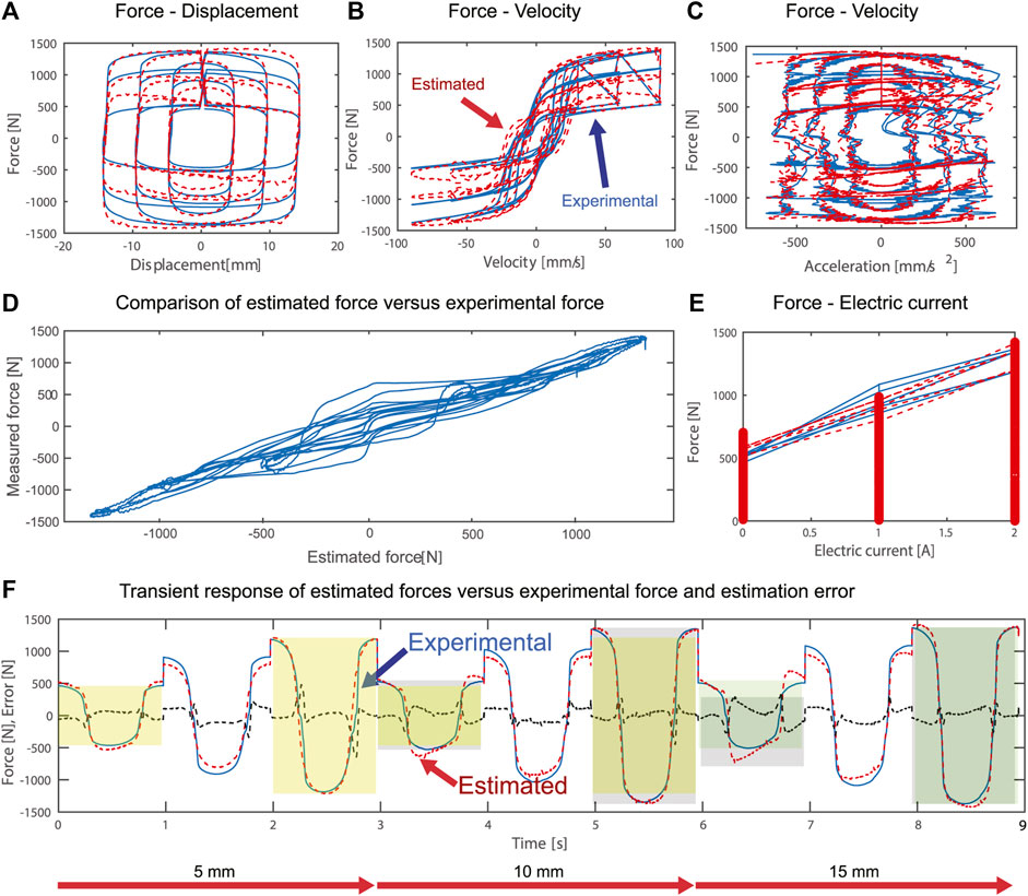
FIGURE 18. Characteristic diagrams, transient response and estimated vs. experimental forces plots for the Complete-Complete MR damper model.

The proposed method of modeling using the generation and classification of p and SA characteristic diagrams fits this specimen, when the pressure is present inside the chambers. The quantitative, Table 14 and qualitative results, Figure 18, provide evidence and validate this proposal.

The characterization of the dynamics and the effect of the control inputs based on the subtraction of the damping forces when the input under study remains constant, allows for better understanding the diagrams, in this case, it has also been used for the pressure, Figure 17. Each input has its own impact on the damping force. An interesting aspect is the appropriateness of the approach to understanding the effect of the pressure variation using the subtracted damping force. It was evidenced that such a pressure effect can be analyzed as an additive component in a further improvement of this method, using some recent results in fault detection of shock absorbers, Hernández-Alcántara et al. (2016).

5 Conclusion

A methodology for the modeling of p and SA shock absorbers based on standard experimental tests has been presented and used with a two degrees of freedom shock absorber. The characteristic diagrams were constructed using experimental data to guide the designer in the development of the structure of the model, starting with a generic equation that introduced a simplified mathematical structure. We experimentally validated the proposal with the specimen. The obtained results had errors below 5%.

The present method needs to be extended to include the modeling of the damping force generated for the variation of internal pressure as control input, so a set of new models will be added for such classification.

Data Availability Statement

The raw data supporting the conclusions of this article will be made available by the authors, without undue reservation.

Author Contributions

JL-S, OS, RM-M and RR-M conceived and designed the analysis. JL-S and JT-M collected the non 2DoF shock absorber data. AS collected the data for the 2DOF MR damper. JL-S and JT-M performed the analysis. JL-S, AS and JT-M contributed data and analysis tools. JL-S wrote the paper.

Funding

This work was supported by a CONACYT Grant 2012-2014, “Programa de Estimulo a la Innovacion” in category “BILATERAL” with grant number 142183, and the 2011 ”Programa de Estimulo a la Innovacion” in category ”PROINNOVA” with grant number 132758.

Conflict of Interest

The authors declare that the research was conducted in the absence of any commercial or financial relationships that could be construed as a potential conflict of interest.

Acknowledgments

The authors want to acknowledge the support from Luc Dugard from Gipsa-Lab, Grenoble Institute of Technology, and Ricardo Prado, Professor in Tecnologico de Monterrey. Also, JL-S wants to thanks to the support from GIPSA-Lab in Grenoble, France.

References

Akutain, X. C., Vinolas, J., Savall, J., and Biera, J. (2006). A parametric damper model validated on a track. Ijhvs 13, 145–163. doi:10.1504/ijhvs.2006.010015

CrossRef Full Text | Google Scholar

Basso, R. (1998). Experimental characterization of damping force in shock absorbers with constant velocity excitation. Veh. Syst. Dyn. 30, 431–442. doi:10.1080/00423119808969459

CrossRef Full Text | Google Scholar

Boggs, C. M. (2009). The use of simulation to expedite experimental investigations of the effect of high-performance shock absorbers. Ph.D. thesis. Blacksburg (VA): Virginia Polytechnic Institute and State University.

Google Scholar

Calvo, J. A., López-Boada, B., Román, J. L. S., and Gauchía, A. (2009). Influence of a shock absorber model on vehicle dynamic simulation. Proc. Inst. Mech. Eng. - Part D J. Automob. Eng. 223, 189–203. doi:10.1243/09544070jauto990

CrossRef Full Text | Google Scholar

Çesmeci, S., and Engin, T. (2010). Modeling and testing of a field-controllable magneto-rheological fluid damper. Int. J. Mech. Sci. 52, 1036–1046. doi:10.1016/j.ijmecsci.2010.04.007

CrossRef Full Text | Google Scholar

Choi, S.-B., Lee, S.-K., and Park, Y.-P. (2001). A hysteresis model for the field-dependent damping force of a magnetorheological damper. J. Sound Vib. 245, 375–383. doi:10.1006/jsvi.2000.3539

CrossRef Full Text | Google Scholar

Codeca, F., Savaresi, S. M., Spelta, C., Montiglio, M., and Leluzzi, M. (2008). “Identification of an electro-hydraulic controllable shock absorber using black-block non-linear models,” in 17 IEEE international conference on control applications, San Antonio, TX, September 3–5, 2008 (New York, NY: IEEE), 462–467.

Google Scholar

Coleman, T. F., and Li, Y. (1996). An interior trust region approach for nonlinear minimization subject to bounds. SIAM J. Optim. 6, 418–445. doi:10.1137/0806023

CrossRef Full Text | Google Scholar

Dixon, J. C. (2008). The shock absorber handbook. West Sussex, United Kingdom: Wiley.

Duym, S. (1997). An alternative force state map for shock absorbers. Proc. Inst. Mech. Eng. - Part D J. Automob. Eng. 211, 175–179. doi:10.1243/0954407971526344

CrossRef Full Text | Google Scholar

Duym, S. W. R. (2000). Simulation tools, modelling and identification, for an automotive shock absorber in the context of vehicle dynamics. Veh. Syst. Dyn. 33, 261–285. doi:10.1076/0042-3114(200004)33:4;1-u;ft261

CrossRef Full Text | Google Scholar

Golinelli, N., and Spaggiari, A. (2015). Design of a novel magnetorheological damper with internal pressure control. Frattura ed Integritaá Strutturale. 9, 13–23. doi:10.3221/igf-esis.32.02

CrossRef Full Text | Google Scholar

Golinelli, N., and Spaggiari, A. (2017). Experimental validation of a novel magnetorheological damper with an internal pressure control. J. Intell. Mater. Syst. Struct. 28, 2489–2499. doi:10.1177/1045389x17689932

CrossRef Full Text | Google Scholar

Guo, S., Yang, S., and Pan, C. (2006). Dynamic modeling of magnetorheological damper behaviors. J. Intell. Mater. Syst. Struct. 17, 3–14. doi:10.1177/1045389x06055860

CrossRef Full Text | Google Scholar

Heo, S.-J., Park, K., and Son, S.-H. (2003). Modelling of continuously variable damper for design of semi-active suspension systems. Ijvd. 31, 41–57. doi:10.1504/ijvd.2003.002046

CrossRef Full Text | Google Scholar

Hernández-Alcántara, D., Tudón-Martínez, J. C., Amézquita-Brooks, L., Vivas-López, C. A., and Morales-Menéndez, R. (2016). Modeling, diagnosis and estimation of actuator faults in vehicle suspensions. Contr. Eng. Pract 49, 173–186. doi:10.1016/j.conengprac.2015.12.002

CrossRef Full Text | Google Scholar

Hong, K.-S., Sohn, H.-C., and Hedrick, J. K. (2002). Modified skyhook control of semi-active suspensions: a new model, gain scheduling, and hardware-in-the-loop tuning. J. Dyn. Syst. Meas. Contr. 124, 158–167. doi:10.1115/1.1434265

CrossRef Full Text | Google Scholar

Joarder, M. N. (2003). Influence of nonlinear asymmetric suspension properties on the ride characteristics of road vehicle. Master’s thesis. Montreal, Canada: Concordia University.

Google Scholar

Kwok, N. M., Ha, Q. P., Nguyen, T. H., Li, J., and Samali, B. (2006). A novel hysteretic model for magnetorheological fluid dampers and parameter identification using particle swarm optimization. Sensor Actuator Phys. 132, 441–451. doi:10.1016/j.sna.2006.03.015

CrossRef Full Text | Google Scholar

Lozoya-Santos, J. d.-J., Hernández-Alcantara, D., Morales-Menendez, R., and Ramírez-Mendoza, R. A. (2015). Modelado de Amortiguadores guiado por sus Diagramas Característicos. Revista Iberoamericana de Automática e Inform. Industrial RIAI. 12, 282–291. doi:10.1016/j.riai.2015.05.001

CrossRef Full Text | Google Scholar

Lozoya-Santos, J., Morales-Menendez, R., Ramirez-Mendoza, R. A., Tudón-Martínez, J. C., Sename, O., and Dugard, L. (2012a). Magneto-rheological damper, an experimental study. J. Intell. Mater. Syst. Struct. 23, 1213–1232. doi:10.1177/1045389X12445035

CrossRef Full Text | Google Scholar

Lozoya-Santos, J. d. J., Morales-Menendez, R., and Ramírez Mendoza, R. A. (2012b). Control of an automotive semi-active suspension. Math. Probl Eng. 2012, 1–21. doi:10.1155/2012/218106

CrossRef Full Text | Google Scholar

Ma, X. Q., Rakheja, S., and Su, C. Y. (2007). Development and relative assessments of models for characterizing the current dependent hysteresis properties of magnetorheological fluid dampers. J. Intell. Mater. Syst. Struct. 24, 487–502. doi:10.1177/1045389X06067118

CrossRef Full Text | Google Scholar

Poussot-Vassal, C. (2008). Commande robuste LPV multivariable de Chassis. Ph.D. thesis. Grenoble, France: INP Grenoble.

Google Scholar

Rakheja, S., and Sankar, S. (1985). Vibration and shock isolation performance of a semi-active on-off damper. J. Vib. Acoust. Stress Reliab. Des. 107, 384–403. doi:10.1115/1.3269279

CrossRef Full Text | Google Scholar

Savaresi, S. M., Bittanti, S., and Montiglio, M. (2005a). Identification of semi-physical and black-box non-linear models: the case of MR-dampers for vehicles control. Automatica. 41, 113–127. doi:10.1016/j.automatica.2004.08.012

CrossRef Full Text | Google Scholar

Savaresi, S. M., Silani, E., and Bittanti, S. (2005b). Acceleration-driven-damper (ADD): an optimal control algorithm for comfort-oriented semiactive suspensions. ASME Trans: J. Dyn. Syst. Meas. Contr. 127, 218–229. doi:10.1115/1.1898241

CrossRef Full Text | Google Scholar

Savaresi, S. M., and Spelta, C. (2007). Mixed sky-hook and ADD: approaching the filtering limits of a semi-active suspension. J. Dyn. Syst. Meas. Contr. 129, 382–392. doi:10.1115/1.2745846

CrossRef Full Text | Google Scholar

Sims, N. D., Holmes, N. J., and Stanway, R. (2004). A unified modelling and model updating procedure for electrorheological and magnetorheological vibration dampers. Smart Mater. Struct. 13, 100–121. doi:10.1088/0964-1726/13/1/012

CrossRef Full Text | Google Scholar

Tudon-Martinez, J. C., Hernandez-Alcantara, D., Amezquita-Brooks, L., Morales-Menendez, R., Lozoya-Santos, J. d. J., and Aquines, O. (2019). Magneto-rheological dampers-model influence on the semi-active suspension performance. Smart Mater. Struct. 28, 105030. doi:10.1088/1361-665x/ab39f2

CrossRef Full Text | Google Scholar

Wang, L. X., and Kamath, H. (2006). Modelling hysteretic behaviour in magnetorheological fluids and dampers using phase-transition theory. Smart Mater. Struct. 15, 1725–1733. doi:10.1088/0964-1726/15/6/027

CrossRef Full Text | Google Scholar

Warner, B. (1996). An analytical and experimental investigation of high performance suspension dampers. Ph.D. thesis. Montreal, Canada: Concordia University.

CrossRef Full Text | Google Scholar

Wright, M. H. (1996). Direct search methods: once scorned, now respectable. Pitman Res. Notes Math. Ser. 191–208.

Google Scholar

Yonaba, H., Anctil, F., and Fortin, V. (2010). Comparing sigmoid transfer functions for neural network multistep ahead streamflow forecasting. J. Hydrol. Eng. 15, 275–283. doi:10.1061/(asce)he.1943-5584.0000188

CrossRef Full Text | Google Scholar