A novel differential evolution algorithm for a flange coupling using ANSYS simulations

1 Introduction

Coupling is a mechanical component that firmly connects the driving shaft and the driven shaft in different mechanisms to rotate together and transmit motion and torque. It can be divided into two types: rigid coupling and flexible coupling. The main difference between the two is that the rigid coupling cannot compensate for the relative displacement between two shafts, while the flexible coupling contains elastic elements that can compensate for the relative displacement of the two shafts. Flange coupling, as a kind of rigid couplings, is able to transmit large torque, with simple structure and low price. Therefore, it is often used in mechanical equipment with stable load and strict alignment of two shafts.

By numerically calculating the torsion stiffness of shaft, Yi et al. (2013) pointed out that the radial thickness and axial length of the flange part and the thickness of the flange have a greater impact on the torsional stiffness of the coupling, compared with the impact from the diameters of both the flange and the bolt coupling hole. Based on the finite element method, Kondru analyzed the reason of possible failure in the contact area of the flange coupling, and further pointed out the way of reducing the failure (Kondru and Suneel, 2015). An optimal flange coupling design for the power transmission system in the DU horizontal belt vacuum filter was carried out, to ensure the material performance and maximum mass reduction (Chandrakant and Anand, 2015; Fan and Zhang, 2018). Moreover, the flange coupling was also numerically optimized, focusing on the shear stress reduction of the bolt (Saurav et al., 2015). Furthermore, Gabbasa and Praveen theoretically designed the structure of the flange coupling, which was validated using ANSYS (Praveen and Prateek, 2017; Gabbasa et al., 2022). Cheng exploited ANSYS to analyze the dynamic characteristics and fatigue life of the bolt flange structure when shaft transmitting torque (Cheng, 2018). Although the numerical methods were largely utilized in the flange coupling system, the optimal design mostly focused on a single objective and was lack of comprehensive analyses of material mass and performance optimization. Therefore, this paper establishes a multi-objective optimization model of the GY-type flange coupling with hinged holes and bolts, aiming at the minimum mass and performance redundancy. The multi-objective differential evolution algorithm was further verified using finite element method.

2 Theoretical considerations

2.1 Multi-objective optimization model of flange coupling

The three-dimensional structure of the flange coupling is shown in Figure 1A. Its components are: the flange coupling (composed of the flange part and the flange part), the bolt coupling part, the key, and the shaft. Usually the materials used in each part are different. The known design conditions are usually: motor power P (KW), speed n (rpm), shaft diameter d (mm), load coefficient k, shaft material, key and bolt material, flange material, bolt diameter d₁ (mm), etc.

FIGURE 1

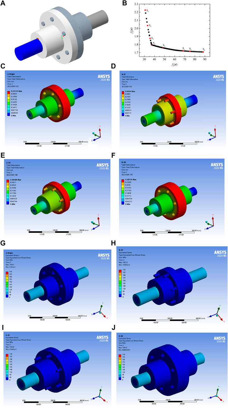
FIGURE 1. (A) Three dimensional model of flange coupling; (B) Pareto curve; (C) Total deformation of origin design; (D) Total deformation of solution S1; (E) Total deformation of solution S5; (F) Total deformation of solution S8; (G) Equivalent stress of origin design; (H) Equivalent stress of solution S1; (I) Equivalent stress of solution S5; (J) Equivalent stress of solution S8.

2.2 Dimensional parameters

The design variable selects the outer diameter D (mm) of the flange, the length L (mm) of the flange, the diameter D₁ (mm) of the bolt distribution circle, the thickness t (mm) of the flange and the number N of the bolts as the design variable. The width and height dimensions of the key are selected according to the diameter of the shaft. The length dimension of the key is taken as the length of the flange and the outer diameter of the flange. The design variable is defined as:

$\left[x_1,x_2,x_3,x_4,x_5\right]=\left[D,L,D_1,t,N\right](1)$

2.3 Constraints

2.3.1 Shear stress constraints of flanges

${\tau }_h=\frac{T_d\times \frac{x_1}{2}}{J}\le \left[{\tau }_h\right](2)$

$T_d=\frac{60\times {10}^{6}P}{2\pi n}\times k(3)$

$J=\frac{\pi \left(x_1^4-d^4\right)}{32}(4)$

where $T_d$ is the design torque. ${\tau }_h$ is the allowable shear stress of the flange material.

2.3.2 Shear stress constraints of bolts

${\tau }_b=\frac{8T_d}{\pi x_3{x}_5{d}_1^2}\le \left[{\tau }_b\right](5)$

where ${\tau }_b$ is the allowable shear stress of bolt material.

2.3.3 Compressive stress constraints of bolts

${\sigma }_c=\frac{2T_d}{x_5{d}_1{x}_4{x}_3}\le \left[{\sigma }_c\right](6)$

where ${\sigma }_c$ is the allowable compressive stress of bolt material.

2.3.4 The shear stress of the key is less than the allowable shear stress

${\tau }_k=\frac{2T_d}{db{x}_2}\le \left[{\tau }_k\right](7)$

where b is the width of the key, ${\tau }_k$ is the allowable shear stress of the key by material.

2.3.5 The extrusion stress of the key is less than the allowable compressive stress

${\sigma }_k=\frac{4T_d}{dh{x}_2}\le \left[{\sigma }_k\right](8)$

where h is the height of the key and the $\left[{\sigma }_k\right]$ is the allowable compressive stress of the key material.

2.3.6 Assembly conditions of adjacent bolt heads

In order not to make adjacent bolt heads interfere with each other and facilitate assembly, sufficient wrench space should be set aside between adjacent bolt heads.

$A\le \frac{\pi x_3}{x_5}(9)$

where A is the distance between the two adjacent bolts of the wrench on the distribution circle, and the query is based on the size of the standard bolt.

2.4 Objective function

2.4.1 Quality objective function of flange coupling

The mass M of the flange coupling is composed of the flange part mass m₁ and the flange part mass m₂.

$m_1=\frac{\pi }{4}\rho \left(x_1^2-d^2\right)x_2(10)$

$m_2=\frac{\pi }{4}\rho \left[\left(D_2^2-x_1^2\right)-x_5{d}_1^2\right]x_4(11)$

where $\rho$ is the density of the flange coupling material. Therefore, the objective function is

$\mathit{min}{f}_1\left(x\right)=m_1+m_2(12)$

2.4.2 Material performance redundancy objective function

Defines the degree of redundancy of material shear performance as the ratio of shear stress to allowable shear stress, i.e.,

$R_{Tm}=\frac{\tau }{\left[\tau \right]}(13)$

R_Tm is close to 1 when the shear stress of the material is close to the allowable shear stress. The degree of redundancy for material compressive performance can be defined as the ratio of the compressive stress to the allowable compressive stress, i.e.,

$R_{Pm}=\frac{\sigma }{\left[\sigma \right]}(14)$

When the compressive stress is close to the allowable compressive stress, the value is close to 1.

Equations 13, 14 show that the definitions of R_Tm and R_Pm, are equivalent to those of safety factors. So, They can represent the strength margin of the material under the stress of real working conditions. The smaller the value, the greater the strength margin. Therefore, the definition of flange coupling performance optimization objective function is:

$\mathit{min}{f}_2\left(x\right)=\frac{{\tau }_h}{\left[{\tau }_h\right]}+\frac{{\tau }_b}{\left[{\tau }_b\right]}+\frac{{\sigma }_c}{\left[{\sigma }_c\right]}+\frac{{\tau }_k}{\left[{\tau }_k\right]}+\frac{{\sigma }_k}{\left[{\sigma }_k\right]}(15)$

To sum up, the multi-objective optimization function model for constructing flange couplings is:

Design variable $x=\left(x_1,x_2,x_3,x_4,x_5,x_6\right)$.

Objective function $\mathit{min}{f}_i\left(x\right)\left(i=\mathrm{1,2}\right)$.

Constraints $g_j\left(x\right)\le 0\left(j=1,\dots ,6\right)$.

The optimization problem is a non-linear optimization problem with two optimization objectives and six constraints.

2.5 A modified multi-objective differential evolution algorithm

Differential Evolution (DE) algorithm (Storn and Price, 1997) is an evolution algorithm proposed by Rainer Storn and Kenneth Price, who used floating-point vector coding to perform random search in continuous space. In recent years, this algorithm has been successfully applied to solve multi-objective optimization problems in engineering (Che and He, 2013; Liu and Lu, 2015; Che et al., 2017; Bai et al., 2022). Studies (Duan, 2021; Fang et al., 2021) show the new computational strategies lead to the improvement of the algorithm effectiveness, so this research exploited the chaotic strategy in the multi-objective optimization algorithm to enhance its computational performances.

2.6 Differential evolution algorithm

The initial population of the difference evolution algorithm is randomly and uniformly generated, and each individual is regarded as a real vector in the D-dimensional search space. If $x_i\left(g\right)$ is the ith individual of the g generation, then $x_i\left(g\right)=\left(x_{i1}\left(g\right),x_{i2}\left(g\right),\dots ,x_{iD}\left(g\right)\right)$, $i\in \left[1,NP\right]$; $NP$ is population size; $g\in \left[1,t_{\mathit{max}}\right]$; $t_{\mathit{max}}$ is the largest evolutionary algebra; $j\in \left[1,D\right]$; and $x_{ij}^L\le x_{ij}\left(g\right)\le x_{ij}^U$, $x_i^U$, $x_i^L$ is the upper and lower bounds of the individual. The individual evolution process is expressed in mathematical language as follows:

${\nu }_{i,j}\left(g+1\right)=\left\{\begin{array}{cc}{x}_{p_1,j}+F\times \left(x_{p_2,j}-x_{p_3,j}\right)& if\left(\mathit{r}\mathit{a}\mathit{n}\mathit{d}\left(\mathrm{0,1}\right)\right.<CRorj=\mathit{r}\mathit{a}\mathit{n}\mathit{d}\left(D\right)\\ x_{i,j}& \mathit{otherwise}\end{array}\right.(16)$

$x_i\left(g+1\right)=\left\{\begin{array}{cc}{\nu }_i\left(g+1\right),& f\left({\nu }_i\left(g+1\right)\right)<f\left({\nu }_i\left(g\right)\right)\\ x_i\left(g\right),& \mathit{otherwise}\end{array}\right.(17)$

In Eqs 16, 17, CR is the crossover rate, which is generally selected between (0, 1); F is the scaling factor, which is generally selected between (0, 2), usually 0.5; rand (0, 1) is a random number that obeys a uniform distribution on (0, 1); $rand\left(D\right)$ is a random integer between $\left[1,D\right]$; $p_1,p_2,p_3$ are integers, and $p_1,p_2,p_3\in \left[1,NP\right]$, $p_1\ne p_2\ne p_3\ne i$; $f\left(x\right)$ is the evaluation function.

2.7 Modified multi-objective differential evolution algorithm

Although the difference evolution algorithm has fewer parameters, each parameter has a significant impact on the optimization ability of the algorithm. The scaling factor F is used to control the degree of influence of the difference vector on the individual, and the size of its value greatly affects the convergence and convergence rate of evolution. When F is small, the development ability of the algorithm is strong, the convergence rate is fast, and it is also easy to make the population converge prematurely to non-optimal solutions; when the value of F is large, it increases the search space of the population and improve the diversity of the population. It is conducive to the algorithm to search for the optimal solution, but the convergence rate is slow. The standard DE algorithm usually uses a fixed scaling factor to set different values according to different problems. The setting of F usually requires certain algorithm experience or multiple attempts.

The reduction of the parameter F effects on the algorithm induces the decrement of user participation, so, the exploitation of Chaos ergodicity prompts F to fall in the range of (0, 1), and hence, reduce the user participation, and balance the convergence rate and global nature of the algorithm. Fu proposed a self-adaption folding chaos optimization method-Fuchs map, and it has stronger chaos characteristics compared with traditional Logistic map, Tent map, etc. (Fu and Ling, 2013). The iteration formula of Fuchs map is

$x_{k+1}=\mathit{cos}\left(\frac{1}{x_k^2}\right)(18)$

Where k is the number of iterations; $x_k\ne 0$ For scaling factor F, first random initialization, Then the scaling factor for each generation is iterated according to Eq. 19.

$F_{k+1}=\mathit{cos}\left(\frac{1}{F_k^2}\right)(19)$

A Modified Multi-Objective Differential Evolution Algorithm (MMODE) is proposed based on the multi-objective difference evolution algorithm. The algorithm flow is as follows

Step 1:. Initialization algorithm parameters and population.

Step 2:. Initialization of file A.

Step 3:. Generate scaling factor F for each generation of evolution according to Eq. 19.

Step 3.1:. Three individuals p1, p2, p3, executive Eq. 15 were randomly selected.

Step 3.2:. Execute the selection operation of Eqs 16, 17.

Step 3.3:. Update the archive file with the newly generated individual. If the new individual is not dominated by the archive set individual, insert it into A, and delete all solutions in A that are dominated by the new individual; if the new individual and the individual in the archive file are mutually dominated and the archive file is not reached The maximum limit is inserted into A. If the archive file A is full, use the archive set pruning strategy to reduce it.

Step 4:. Perform the following steps for each individual:

Step 5:. Evolutionary algebra plus 1, to determine whether the convergence condition is reached, if not, then go to Step 3; otherwise, the output file A, Pareto optimal solution set.From the flow of the MMODE algorithm, it can be seen that the main difference between the MMODE algorithm and the MODE algorithm is that in each iteration, a different scaling factor F is generated, so it is the same as the MODE in time complexity. The MMODE algorithm still adopts the selection strategy of “survival of the fittest,” so its convergence is also the same as the MODE algorithm, both of which are progressive convergence.

3 Results and discussion

3.1 Pareto solution

The flange couplings used to design a certain equipment have a transmission power of 90.0 KW and a speed of 250 rpm. The material of the shaft is 40C8, and the diameter of the shaft is 80 mm; the material of the key and bolt is 30C8, and the nominal diameter of the bolt is 18 mm, and the number is 4. The material of the flange couplings is gray cast iron. The load factor is 1.5. According to the diameter of the shaft, the size of the key is selected to be 22 mm wide and 14 mm high. The safety factor of the shaft, key and bolt is 2.5, and the safety factor of the coupling is 6. According to the above conditions and the performance of the material, it is obtained: $\left[{\tau }_h\right]=16.67N/m{m}^2$, $\left[{\tau }_b\right]=\left[{\tau }_k\right]=80N/m{m}^2$, $\left[{\sigma }_c\right]=\left[{\sigma }_k\right]=240N/m{m}^2$.

The MMODE algorithm is used to solve the problem. The algorithm parameters are set to 100 for the population size, 100 for the number of archived sets, 0.3 for the crossover probability, and 800 for the evolutionary algebra. Set the search range of the variable to $D\in \left[\mathrm{140,180}\right]$, $L\in \left[\mathrm{100,140}\right]$, $D_1\in \left[\mathrm{220,260}\right]$, $t\in \left[\mathrm{30,50}\right]$, $N\in \left[\mathrm{4,6}\right]$ and N is rounded during calculation. The Pareto leading edge obtained is shown in Figure 1B. The Pareto solution is shown in Table 1.

TABLE 1

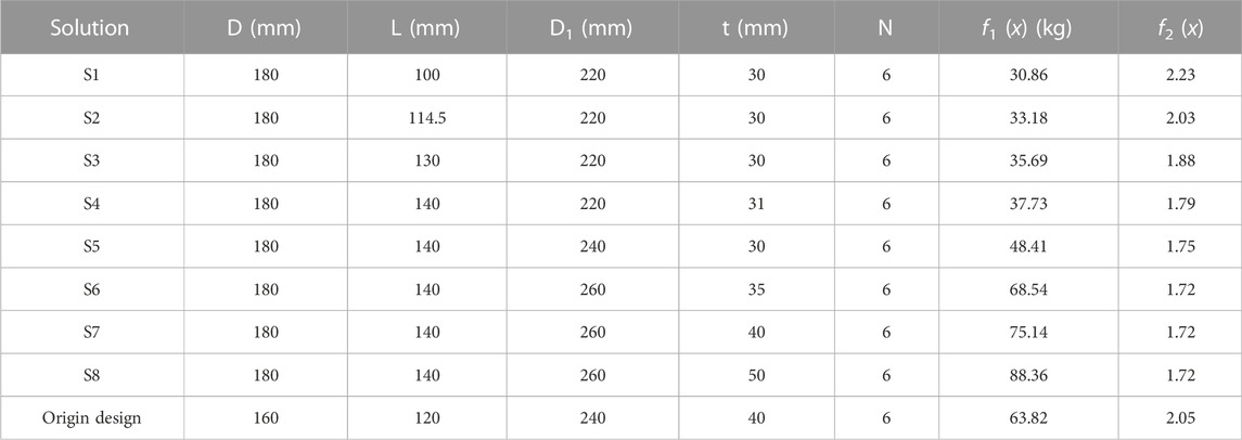
TABLE 1. The obtained optimized solution.

In Figure 1B, the Pareto leading edge obviously has a corner at point S4. On the left side of the inflection point, the value of the performance evaluation function drops faster, while the mass function increases slowly; on the right side of the inflection point, the performance evaluation function changes little, but the mass increases faster. Judging from the data in Table 1, the main difference between the four solutions S1∼S4 is that the size of the flange portion, the size of the flange is dominated by length changes, and the greater the length of the mass; and the difference between the solutions S4∼S8 is that the size of the flange portion, the size of the bolt distribution circle determines the outer diameter of the flange, the larger the size of the distribution circle, the larger the size of the flange, the greater the thickness of the flange, the greater the mass, the size of the flange has little effect on the overall performance, but it has a greater impact on the mass. Compared with the original design, the optimized solutions are larger in the diameter of the flange than the original design. The following is an analysis of whether the solutions obtained above can meet the design requirements through the finite element method.

3.2 Finite element simulations

Creo was used to build and assemble various parts of the flange coupling model. ANSYS 2020 was exploited for finite element simulations. Material density is set to 7,850 × 10⁻⁹ (kg/mm³). The Poisson’s ratios of materials 40C8 and 30C8 are set to 2 × 10⁵ (MPa) and Gray cast iron is set to 1 × 10⁵ (MPa). The Young’s modulus of materials 40C8, 30C8, and Gray cast iron are set to 0.27, 0.3, and 0.23, respectively. The mesh size is set to 5 mm. Double step are applied for loading: the first step is to apply a pre-tightening force of 1000 N on each bolt, while the second step is to apply the design torque T_d.

Figures 1C–F show the comparison of the total deformation of the original design scheme and the Pareto solutions S1, S5, and S8. Figures 1G–J shows the comparison of the equivalent effect forces of the original design scheme and the Pareto solutions S1, S5, and S8.

In present study, the theory adopted to calculate permissible stress is maximum shear stress theory. The maximum shear stress theory (also called the Tresca theory), it equates the maximum shear stress for a general state of stress to the maximum shear stress obtained when the tensile specimen yields. The maximum shear stress theory which is shown in Eq. 20.

${\tau }_{\mathit{max}}=\frac{1}{2}\left({\sigma }_1-{\sigma }_3\right)\ge \frac{1}{2}{\sigma }_s(20)$

Where${\sigma }_1$ = Maximum principal stress

${\sigma }_3$ = Minimum principal stress

${\sigma }_s$ = Maximum shear stress

The maximum principal stress of S1, S5, S8, and original design are 136.3 MPa, 137.73 MPa, 127.17 MPa, and 132.32 MPa. The minimum principal stress of S1, S5, S8, and original design are −148.44 MPa, −148.78 MPa, −146.97 MPa, and −144.91 MPa. The maximum shear stress of S1, S5, S8, and original design are 97.70 MPa, 95.073 MPa, 97.243 MPa, and 94.557 MPa. It can be seen from the results that the optimization range of performance and mass is greater than the variation range of maximum principal stress, minimum principal stress and maximum shear stress. Therefore, the optimization results meet the certain stress requirements which can facilitate the optimization design and applied to actual production.

4 Conclusion

In this research, an improved multi-objective difference evolution algorithm was applied for a flange coupling model, using finite element simulations. The Pareto solution was achieved for future engineering structural designs. The conclusion are drawn as follows:

(1) The addition of flange thickness leads to the mass increment of the coupling frame, but The size of the flange takes less effect on the overall performance.

(2) The optimization of the structure dimension and flange coupling mass leads to the evident reductions, which fulfils the special requirements of engineering performance, and decrease the material mass.

(3) Under the design conditions, the greater mass of the flange coupling results in the larger strength margin of the material, while the fluctuation of the strength margin is less evident than the mass change.

(4) The modified multi-objective optimization evolution algorithm can be utilized for the targeted flange coupling model, which paves the way of the future coupling structure design. Moreover, the Pareto solution was found to be superior for the optimization problems in real practices, although its universality needs further experimental investigations.

Data availability statement

The raw data supporting the conclusion of this article will be made available by the authors, without undue reservation.

Author contributions

QL was responsible for the investigation, established the multi-objective optimization model of flange coupling, developed the software, and edited the paper. YJ was responsible for the three dimensional model construction and finite element analysis, and acquiring funding and reviewed the paper.

Funding

This work has been supported by the Key scientific research projects of colleges and universities in Henan Province (Grant No. 22B460032 and 23B460016).

Acknowledgments

The research work of this paper has been strongly supported by Zhengzhou Vocational and Technical College, which has provided equipment and funds for the research, and thanks to the help of other colleagues in Henan Industrial Robot Application Engineering Research Center.

Conflict of interest

The authors declare that the research was conducted in the absence of any commercial or financial relationships that could be construed as a potential conflict of interest.

Publisher’s note

All claims expressed in this article are solely those of the authors and do not necessarily represent those of their affiliated organizations, or those of the publisher, the editors and the reviewers. Any product that may be evaluated in this article, or claim that may be made by its manufacturer, is not guaranteed or endorsed by the publisher.

References

Bai, H., Yuan, Q., and Wang, X. (2022). Application of improved differential evolution algorithm in constrained optimization problems. Modul. Mach. Tool. andAutomatic Manuf. Tech. 1, 43–47.

Google Scholar

Chandrakant, M., and Anand, M. (2015). Design and analysis of flange coupling. Int. J. Of Eng. Res. 5, 89–93.

Google Scholar

Che, L., and He, B. (2013). Differential evolution algorithm of multiobjective optimization for Cylindrical gear transmission. J. Of Mech. Transm. 37, 61–66.

Google Scholar

Che, L., Yi, J., and Du, L. (2017). Multi-objective optimal design of Flapping-Wing mechanism formed by A single-Crank and Double-Rockers Linkage. J. Of Mach. Des. 34, 91.

Google Scholar

Cheng, S. (2018). The characteristics of torsional Vibration and the Loss of fatigue life of flange coupling. Bei Jing,China: North China Electric Power University. Master Thesis.

Google Scholar

Duan, W. (2021). Improved differential evolutionary algorithm and its Application in mechanical optimization Master. Shanghai, China: Shanghai University Of Engineering Science.

Google Scholar

Fan, J., and Zhang, Y. (2018). Optimization design of the Du-type horizontal- belt vacuum filter. Mochine Des. And Res. 34, 194–197.

Google Scholar

Fang, J., Ji, Y., and Zhao, X. (2021). Opppsition-based differential evolution algorithm with Gaussian distribution Estimation. J. Of Henan Normal Univ. Nat. Sci. Ed. ) 49, 27–32.

Google Scholar

Fu, W., and Ling, C. (2013). An adaptive iterative chaos optimization method. J. Of Xi' an Jiaot. Univ. 47, 33–38.

Google Scholar

Gabbasa, A., Daas, O., and Assaleh, T. (2022). Theoretical design and stress analysis for flange coupling. Sci. J. Of Appl. Sci. Of Sabratha Univ. (9), 100–109.

Google Scholar

Kondru, N., and Suneel, D. (2015). Failure analysis of flange coupling with two different materials. Int. J. Of Eng. Res. 04, 587–589.

Google Scholar

Liu, W., and Lu, Q. (2015). Multi-objective optimization design of Sleeve Roller Chain transmission based on differential evolution algorithm. J. Of Mech. Transm. 39, 77–80.

Google Scholar

Praveen, K., and Prateek, Y. (2017). Structural analysis of rigid flange coupling by finite element method. Int. J. Of Eng. Sci. Technol. 6, 164–170.

Google Scholar

Saurav, R., Debayan, D., and Pawan, J. (2015). Design and Strss-analysis of A rigid flange coupling using Fem. Int. J. Of Innovative Res. Sci. Eng. And Technol. 4, 9599–9606.

Google Scholar

Storn, R., and Price, K. V. (1997). Differential evolution—a simple and efficient heuristic for global optimization over continuous spaces. J. Glob. Optim. 11, 341–359.

CrossRef Full Text | Google Scholar

Yi, Y., Sun, J., and Liang, X. (2013). Torsional stiffness and Sensitivity analysis of non-standard flange coupling. J. Of Mech. Transm. 37, 62–64.

Google Scholar