Benchmark Simulations of Dense Suspensions Flow Using Computational Fluid Dynamics

1 Introduction

Dense granular suspensions, such as concrete, toothpaste, blood and many more, are commonly used in both industry and research. Also important biological and chemical problems can be described this way (Khan et al., 2020; Sultan et al., 2020). The reliable description and modeling of those substances is important to reduce costs, processing times and to generate high quality products. Concrete is the most widely used building material, which contains both a non-Newtonian matrix and granular constituents, thus showing a complex rheology (Toutou and Roussel, 2007). For the modelling of dense suspensions, not only the careful determination of the rheological model parameters is of great importance (Park et al., 2005; Choi et al., 2014; De Schutter and Feys, 2016), but also the choise of the apropriate material model (Dean et al., 2007; Roussel and Gram, 2014; Li et al., 2021).

The granular nature of those materials makes it difficult to determine rheological data. Also air inclusions may lead to complicated rheological behavior during processing (Gálvez-Moreno et al., 2019). Due to the complex nature of this type of suspensions, it is hardly possible to measure and determine reliable and very accurate rheological properties using the available measuring devices. It is known that the material can segregate during shear (Spangenberg et al., 2012; Secrieru et al., 2018). Especially for concrete, this behavior is of great importance for the material transport (Fataei et al., 2020).

Additionally, different models exist to describe the complex time and shear dependent rheology. Among them the Herschel-Bulkley model and the Bingham model (Bird et al., 2002) are widely used to determine the rheological properties of dense suspensions. The models of Jop et al. (2006) and Schaeffer (1987) are some of the most famous models used in case of granular materials. The accuracy of the models used, the boundary conditions as well as the assumptions behind their derivations are different; therefore, the selection of the model influences both the rheological data and the numerical solution. Extended models also include wall roughness and lubrication (Talon et al., 2014).

Same as analytical methods, there exist many different numerical methods to simulate the complex flow behavior of materials. In the field of Computational Fluid Dynamics (CFD), the Finite Volume Method (FVM), the Finite Element Method (FEM) and Smoothed Particle Hydrodynamics (SPH) are used in particular. For each of these methods a number of commercial and open-source software packages exist. In this paper we will use Ansys Fluent¹ and OpenFOAM² on the side of the FVM, COMSOL (COMSOL, 2019) for FEM and the SPH implementation HOOMD-blue.sph (Osorno et al., 2021) in the molecular dynamics tool HOOMD-blue (Anderson et al., 2008; Glaser et al., 2015). The software packages used for this benchmark are summarized in Table 1.

The rheological properties of a granular material in a non-Newtonian matrix were determined and the flow behavior will be modeled numerically with different software packages, Table 1. The material used is described in section 2.1. The numerical results are compared extensively with each other with respect to their quality.

In summary, the main objectives of this paper are divided into the following two parts:

1) A study on the regularization of the various models used in this work.

2) A comparison of different software packages in the simulation of a dense suspension flow under two different boundary conditions.

This study aims to guide researchers to select suitable methods and strategies for modelling dense suspensions and even to give an insight into and highlight the difficulties and limitations. In this paper, in addition to applying commercial and open-source grid-based computational methods for dense suspension simulations, a grid-free simulation software package is used to compare the numerical outputs obtained by a wider range of software packages.

TABLE 1

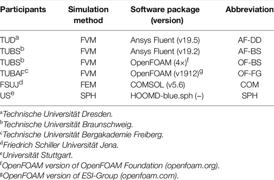
TABLE 1. Software packages used in this benchmark.

2 Benchmark Setup

2.1 Description of the Benchmark Problem

For the benchmark a dense granular suspension was used that was already described for the investigation of concrete like materials Haustein et al. (2020); Mechtcherine et al. (2020). This model concrete is composed of a bidisperse mixture of spherical glass beads. Here, 30% of the particles have a diameter of 0.5 mm and 70% have a size of 1 mm. The liquid model cement used in the suspension is a shear thinning yield-stress liquid based on Carbopol®. The material is refractive index matched with Thiodiethanol, and was designed to behave similar to concrete. Details can be found in Auernhammer et al. (2020). The transparency allows the material to be examined during flow using the Particle Image Velocimetry (PIV) method. In this way, temporally and spatially fully resolved flow profiles of the suspension are obtained, from which the rheological properties during pumping can be determined. Details of the measurement can be found in the literature (Haustein et al., 2020).

For this benchmark, a representative measurement is chosen and the rheological parameters are determined. In a typical measurement, a pressure drop of Δp = 67.2 kPa is measured between two pressure sensors with a distance of L = 1.47 m. The resulting average flow velocity is $\bar{u}=$0.27 m s⁻¹. Please note that in all further sections only the velocity component in the direction of flow (axial direction) is considered and for this reason the notation is changed from vector to scalar.

The rheology of the model concrete mentioned above can be described with the Bingham model:

$\tau ={\tau }_0+{\mu }_p\dot{\gamma }(1)$

with the scalar shear stress τ, the shear rate $\dot{\gamma }$, the yield stress τ₀ and the plastic viscosity μ_p.

By evaluating the flow profiles and fitting with the Bingham model, the dynamic viscosity μ_p = 0.91 Pa s and the yield stress τ₀ = 87.71 Pa can be determined. The derived rheological properties, flow quantities and the basic geometry of PulsaCoP are used as input for numerical simulations in this benchmark. The effective density of the material is given as ρ_eff = 1,560 kg m⁻³.

This flow configuration can be expressed in terms of dimensionless numbers, which are Reynolds Number Re and Bingham Number Bn:

$Re=\frac{{\rho }_{eff}\bar{u}D}{{\mu }_p}\mathrm{a}\mathrm{n}\mathrm{d}Bn=\frac{{\tau }_{0}D}{{\mu }_p\bar{u}},(2)$

Thus Re∼9 and Bn∼7 for all configurations shown in this benchmark. Please note that a variation of those parameters is not in the scope of this study, but is extensively analyzed in Mehmood et al. (2020).

2.2 Numerical Setup

Multiple numerical methods where used for this benchmark as described above. The goal of all those approaches is to solve the mass and momentum conservation equations in the case of an incompressible laminar flow (Bird et al., 2002):

$\nabla \cdot \vec{u}=0(3)$

${\rho }_{eff}\frac{\partial \vec{u}}{\partial t}+{\rho }_{eff}\left(\vec{u}\cdot \nabla \right)\vec{u}=-\nabla p+\nabla \cdot \mathit{\tau }(4)$

with the flow velocity $\vec{u}$, the effective density of the suspension ρ_eff, the pressure p and shear stress tensor τ. It should be noted that the approach for the solution differs between the numerical methods. While FVM and FEM depend on a mesh, the SPH method allows a mesh-free calculation. The interested reader is also referred to Mandal et al. (2018) for an extensive discussion of a benchmark comparing FEM and FVM in granular materials under shear. Furthermore, benchmarks of numerical simulations of Bingham fluids in lid-driven square cavity were given by Mitsoulis and Zisis (2001). A pure FEM benchmark for this kind of fluid is given by Mehmood et al. (2020).

Also numerical issues like the regularization of the models are investigated for the different software packages. For a mathematical and physical investigation of this process, for example, Frigaard and Nouar (2005).

2.2.1 Geometry

As a benchmark, a small, well-defined section within the PulsaCoP system is numerically described. Here it is useful to model the straight segment of the measuring section without elbow and reservoir. Within the 1.47 m long measuring section with a radius R = 0.01 m, the mean flow velocity, the velocity profile and the pressure loss Δp = p₂−p₁ can be investigated very precisely. A simplified sketch of the setup is shown in Supplementary Figure S1.

TABLE 2

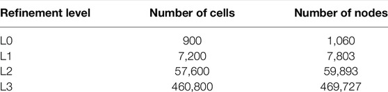
TABLE 2. Refinement levels used for the numerical simulations (grid-based).

Block-structured meshes are created with the Ansys ICEM CFD software. Different refinement levels will be chosen to study the mesh independence, compare the convergence and performance of the software packages. Based on a basic mesh L0 with 900 cells, the next refinement levels are obtained by splitting the cells in each direction. Thus, level 1 (L1) contains 900 ⋅ 8¹ cells and so on. The different levels as well as important mesh properties are given in Table 2. The L0 mesh and the L3 mesh are shown in Supplementary Figure S2. This type of mesh (Table 2) is used in all mesh-dependent software packages.

TABLE 3

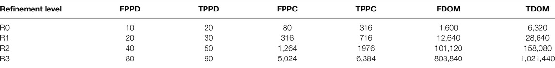
TABLE 3. Refinement levels used for the SPH simulations showing fluid particles per diameter (FPPD), total particles per diameter (TPPD), fluid particles per cross section (FPPC), total particles per cross section (TPPC), total number of fluid particles in the domain (FDOM) and total number of particles in the domain (TDOM).

While SPH is a meshless method, it therefore requires a different type of discretization. To ensure consistency and comparability to the simulations discretized by the mesh-free SPH method, also four different resolutions are used. The lowest resolution R0 contains 10 fluid particles over the pipe diameter (FPPD), Table 3. For each further simulation, the fluid particle number is doubled over the pipe diameter resulting in refinement levels R1 with 20 up to R3 with 80 particles over the diameter, see also Supplementary Figure S3. Additionally to the resolution of the fluid particles as common for the SPH method ghost particles are used to ensure the no-slip condition at the pipe walls. In flow direction, periodic boundary conditions are used for this benchmark, as is generally often the case with the SPH method due to its straightforward implementation. Thus it is difficult to compare the total particle count with the number of cells in the mesh-based methods, since the domain has only a certain length to ensure the non-occurrence of stability issues. However, to explicitly mention the number of fluid and the sum of fluid and ghost particles used in these simulations, the number of particles is depicted in Table 3.

TABLE 4

TABLE 4. Overview of simulation setups including the boundary conditions (BC). The zero-gradient BC is abbreviated as zG.

2.2.2 Boundary Conditions

Various boundary conditions were examined for the investigations within the benchmark. For all cases, no-slip boundary conditions at the pipe wall for velocities and zero gradient (zG) boundary conditions for pressure are applied. In the first case, a constant inlet velocity in axial direction u₀ was specified as inlet boundary condition (denoted as cv). A zero gradient boundary condition was assumed for the velocity at the outlet. In this case, the pressure at the inlet was also given as a zero gradient boundary condition and a constant pressure of 0.0 Pa relative to ambient pressure at the outlet was given. The selection of the boundary conditions was based on the measurements on the PulsaCoP apparatus, Table 4.

In the second case, a constant pressure gradient from the measurement was used to define the boundary conditions (denoted as cp). The inlet pressure was set to a constant value of p₁ and the outlet pressure to the value p₂ = 0.0 Pa. The zero gradient boundary conditions are used for inlet and outlet. It has to be noted, that for the simulations with OpenFOAM the pressure as well as the shear stress is normalized to the effective suspension density ρ_eff = 1,560 kg m⁻³.

In case of OpenFOAM, the velocity field was initialized with 0.27 m s⁻¹ for the cv setup and with 0.0 m s⁻¹ in the cp setup. The initial pressure field was set in both cases to 0.0 Pa. In the Ansys Fluent group, the velocities as well as pressure field were initialized using standard initialization method provided in Ansys Fluent. This initialization method was used in both the cv and cp cases. In COMSOL, the initial values for pressure were set to 0 Pa and for velocity to 0 m s⁻¹.

For the simulations using SPH only the cp case was simulated. Therefore the given pressure boundary condition was converted into a body force of 29.29 m s⁻² in direction of the flow (along the channel length) by considering the pressure difference and channel length. Due to the standard periodic boundary conditions of the code and the absence of inflow/outflow boundary condition, the simulation of the cv case was not performed, since it would require the simulation of non periodic boundary conditions and thus be contrary to the actual strength of the simplicity of the method.

2.2.3 Regularization Models

Since the Bingham behavior in the limit $\dot{\gamma }\to 0$ cannot be captured in a CFD simulation, modified approaches have been implemented in the software packages, namely the bi-viscous and the Bingham-Papanastasiou model (short Papanastasiou model). Both approaches require a regularization procedure to represent the transition from sheared to unsheared (plug flow) region. Each of them is briefly explained below.

2.2.3.1 Bi-Viscous Model

There are two distinct conditions, sheared and unsheared (plug flow) regions, in the flow behavior, which can be determined using the following formulation (Lipscomb and Denn, 1984; O’Donovan and Tanner, 1984).

$\begin{array}{cc}\hfill {\mu }_{app}={\mu }_p+\frac{{\tau }_0}{\dot{\gamma }}& \text{for}\left[\dot{\gamma }>{\dot{\gamma }}_c\right]\hfill \\ \hfill {\mu }_{app}={\mu }_0={\mu }_p+\frac{{\tau }_0}{\dot{{\gamma }_c}}& \text{for}\left[\dot{\gamma }\le {\dot{\gamma }}_c\right]\hfill \end{array}(5)$

with the shear rate $\dot{\gamma }$, the yield stress τ₀, the plastic viscosity μ_p, the shear stress τ, the initial viscosity μ₀, the apparent viscosity μ_app and the critical shear rate ${\dot{\gamma }}_c$. The regularization using the bi-viscous model is presented by varying the critical shear rate ${\dot{\gamma }}_c$, below which the kinematic viscosity ν = η_app/ρ_eff can be considered constant ν₀.

2.2.3.2 Bingham-Papanastasiou Model

The Bingham-Papanastasiou model, introduced by Papanastasiou (Papanastasiou, 1987), is a modification of the Bingham plastic model, which is developed by introducing a regularization parameter m to overcome its discontinuity for $\dot{\gamma }\to 0$.

${\mu }_{app}={\mu }_p+\frac{{\tau }_0}{\dot{\gamma }}\left(1-e^{-m\dot{\gamma }}\right)(6)$

The equation is valid for both regions of material behavior, yielded and unyielded (plug flow). Thus it avoids an explicit solution for the location of the yield surface Mitsoulis (2007); Pierre et al. (2020a); Pierre et al. (2020b). The Newtonian fluid behavior is recovered when m = 0 and more importantly, the limit of m→∞ is entirely equivalent to the ideal Bingham model. In this work, the exponent m was varied to have the possibility to study the regularization of the model and its effect on the accuracy of the numerical results reported by different software packages.

2.2.4 Discretization Schemes

All discretization schemes were chosen to be of second order in space, except for a few simulations performed with COMSOL due to stability reasons. According to the goal of the work, all simulations were carried out under steady-state conditions in the context of this benchmark. It should be noted that the number of iterations required to achieve convergence at different boundary conditions, the convergence criteria and solution methods used, differ between the different software packages. See also Supplementary Table S1 in supplementary material.

2.2.5 Software Packages

2.2.5.1 Ansys Fluent

In this study, the commercial software package Ansys Fluent is used with two different versions, v19.5 at TUD and v19.2 at TUBS, Table 1.

User-defined Functions (UDFs) allow us to customize Ansys Fluent and can boost its capabilities and standard features significantly [for details refer to (UDF, 2006)]. In this study, two separate UDFs were written and implemented into Ansys Fluent. 1) a UDF for the bi-viscous model (Eq. 5) to determine the kinematic viscosity of the model material. According to the goal, different critical shear rates used to have an investigation on the regularization of the model. In each case, the maximum initial apparent viscosity was calculated from the maximum kinematic viscosity and was set in the written UDF, resulting in a critical shear rate of ${\dot{\gamma }}_c$. 2) a UDF for the Papanastasiou (Eq. 6) model with a regularization parameter m. Similar to case 1, a regularization study was performed. In case 2, the regularization parameter m was changed to study its effect on numerical results.

2.2.5.2 OpenFOAM

One of the software packages used to model the flow with the Finite Volume Method (FVM) is the open source software package OpenFOAM. This well tested CFD software allows to solve complex flow problems including chemical reactions, solid mechanics and many more. The original software FOAM was published 1989 and developed further into different branches. For the benchmark shown here the 1912 version of the ESI group was used at TUBAF and OpenFOAM 4.x from the OpenFOAM Foundation was used at TUBS. As solver simpleFoam is used in both cases. The calculations were performed at the High Performance Computing Center of the TU Bergakademie Freiberg and at High Performance Computing Center Phoenix of the TU Braunschweig.

2.2.5.3 COMSOL

COMSOL is a commercial Finite Element Method (FEM) software package which is able to find the numerical answer for a vast amount of physical phenomena and the coupling between them. It has already been used in the concrete rheological field, e.g., to study the optimal rheological properties of SCC for formwork filling in the presence of bars (Alfi et al., 2013), to analyse the degree of plug flow when pumping (Jacobsen et al., 2009), to predict the effect of temperature and cement hydration on the rheological behavior of cement back filling (Wu et al., 2013), and to evaluate the flow behavior in a drilling shaft (Jeyaraj, 2018).

We use the CFD module of COMSOL to solve the conservation of mass and momentum (Navier-Stokes) equations in the two benchmark exercises (cv and cp). The Galerkin method is applied which implies that test and basic functions are the same. The basic functions are composed by Lagrange elements. The mesh is imported into COMSOL by first exporting the provided Ansys ICEM CFD.msh file as.vtk file using OpenFOAM, and later as.bdf file using Gmsh (Geuzaine and Remacle, 2009). The solution of the bi-viscous model was carried out with first order elements, since the convergence for the developed model was better.

2.2.5.4 HOOMD-Blue.sph (SPH)

Smoothed Particle Hydrodynamics (SPH) is a Lagrangian particle method, first formulated by Gingold and Monaghan (1977) and Lucy (1977) for applications in astrophysics. Later SPH was successfully applied to a wide variety of problems in other fields of physics and mechanics, such as fluid dynamics and solid mechanics or even coupled problems. SPH offers several advantages for the numerical simulation of fluid flows with varying Reynolds numbers, due to its Lagrangian formulation. Furthermore, the meshless nature of SPH renders the setup of boundary value problems, for instance the discretization of XRCT-generated microstructures, comparatively easy compared to mesh-based methods.

Using the particle infrastructure of the highly optimized MPI-CPU-GPU simulation toolkit HOOMD-blue (Anderson et al., 2008; Glaser et al., 2015), we use the general SPH toolkit HOOMD-blue.sph which has been shown great scaling results on both GPU and CPU (Osorno et al., 2021). Besides Newtonian fluid flow the implementation for the non-Newtonian fluid flow includes both, the regularized Papanastasiou-Bingham model as well as the bi-viscous model. Since a more detailed view of the method and the implementation is out of the scope of this work, the reader is referred to Osorno et al. (2021) and Kijanski et al. (2020) for further details.

TABLE 5

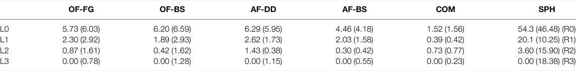
TABLE 5. Mesh accuracy: percentage error of velocity profile of different software packages compared with the highest refinement level L3 and the analytical solution in brackets. For SPH, the results are compared with the refinement level R3.

3 Results

The results achieved from the above-mentioned simulations from different software packages are presented, compared and discussed. The velocity and viscosity profiles are extracted from the center of the grid-cell and shown over the normalized radius r/R_C, where R_C is the cylinder radius of 0.02 m.

3.1 Mesh Convergence

To be able to compare the results of different numerical methods, a mesh independence study was performed. For this purpose, the velocity profiles with the different grid accuracies are compared using the functional (Mandal et al., 2018):

${\xi }_{ij}=100.0\sqrt{\frac{{\int }_{y=-R}^{y=R}{\left({\varphi }_i-{\varphi }_j\right)}^2\mathrm{d}y}{{\int }_{y=-R}^{y=R}{\varphi }_i^2\mathrm{d}y}}(7)$

which gives the percentage deviation between two profiles ϕ_i and ϕ_j of a flow quantity. The flow quantities analyzed here are the velocity and the viscosity, thus ϕ ∈ (u, ν). This allows to quantify the error between the flow profile i and the reference profile j, which can be either a higher refinement level or an analytical solution. Please note the usage of the scalar velocity u as axial component of $\vec{u}$.

The velocity profile of a Bingham-type fluid in a straight pipe can be calculated analytically as (Giesekus, 1994):

$u\left(r\right)=\left\{\begin{array}{ccc}\frac{\mathrm{\Delta }p}{4{\eta }_{app}L}{\left(R-\frac{2{\tau }_{0}L}{\mathrm{\Delta }p}\right)}^2\hfill & \hfill \text{for}& \hfill r\le \frac{2{\tau }_{0}L}{\mathrm{\Delta }p}\\ \frac{\mathrm{\Delta }p}{4{\eta }_{app}L}\left(\left(R^2-r^2\right)-\frac{4{\tau }_{0}L}{\mathrm{\Delta }p}\left(R-r\right)\right)\hfill & \hfill \text{for}& \hfill r>\frac{2{\tau }_{0}L}{\mathrm{\Delta }p}\end{array}\right.(8)$

The viscosity can be calculated with Eqs 5, 6 for the bi-viscous model and the Bingham-Papanastasiou model, respectively, with the shear rate

$\dot{\gamma }=\frac{\text{d}u}{\text{d}r}(9)$

deduced from the analytical/numerical velocity profile u(r).

The results are shown in Table 5. The results of Eq. 7 for the different refinement levels with the finest level L3 are given as well as the deviation from the analytical solution in brackets. The data refers to the velocity profiles of a simulation with the Bingham-model (${\dot{\gamma }}_c=$0.01 s⁻¹, ν₀ = 5.63 m² s⁻¹). The line plots u(r) were extracted for a simulation with constant inlet velocity in all cases except for the SPH simulation. The HOOMD-blue.sph software is not able to use the constant velocity inlet boundary, thus the mesh convergence was determined for a constant pressure loss (cp). As a representative example, the velocity profiles for the different refinement levels with OpenFOAM (OF-FG) are shown in Supplementary Figure S4.

It can be seen, that for all software packages using a fixed mesh the error in the velocity profile is below 1.5% between L2 and L3 for the mesh-based software. Therefore, all further results are discussed using the L2 mesh, which shows a good compromise of accuracy and computational speed. In case of the mesh-less SPH method the error is slightly higher compared to FVM and FEM.

TABLE 6

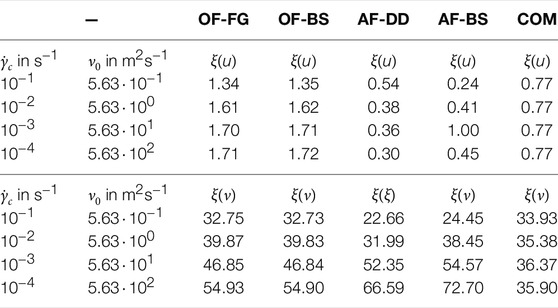
TABLE 6. Comparison of the percentage error of the velocity ξ(u) and the viscosity ξ(ν) compared to the analytical solution of the bi-viscous model (Eq. 8) and (Eq. 5) for the different regularization parameters (critical shear rate ${\dot{\gamma }}_c$ and critical kinematic viscosity ν₀, respectively). All simulations were run for refinement L2 and constant velocity inlet cv.

3.2 Regularization With Constant Velocity Inlet Boundary Condition

In this section, the investigations on regularization of both models explained in Section 2.2.3 are reported for the constant velocity inlet (cv) boundary condition. All investigations shown here were performed with refinement L2. The error ξ was determined in comparison with the analytical solutions for the velocity profile u(r) and the viscosity ν by using the numerical values taken directly from the CFD package.

3.2.1 Bi-Viscous Model

The comparison of the velocity profiles and the viscosity profiles of the bi-viscous model with the analytical solution is summarized in Table 6. Also a representative example for the velocity profiles with OpenFOAM is shown in Supplementary Figure S5.

It can be observed that the results for the velocity profiles show a very small error compared to the analytical solution. In the case of both OpenFOAM versions the error is increasing with increasing ν₀. Thus, a higher regularization parameter leads to a decrease in the accuracy of the velocity profile. Also, the deviations of the different versions is very close to each other. In contrast, the error is clearly decreasing with increasing ν₀ in Ansys Fluent (DD). For the results of Ansys Fluent (BS) no clear tendency can be observed. Furthermore, clear differences between the Ansys Fluent versions can be observed. In COMSOL, the error remains constant for all the different regularization parameters. The best results were achieved with Ansys Fluent (DD) with a high ν₀.

The deviations of the numerical results for viscosity from the analytical solutions, on the other hand, are significantly higher. The error here is in some cases higher than 50%. A comparison of the viscosities for the different regularization parameters ν₀ is also given in Supplementary Figure S6 for the solution with OpenFOAM.

Both Ansys Fluent versions as well as both OpenFOAM versions clearly show a rising error with increasing regularization parameter ν₀. Interestingly, for COMSOL only small differences with no clear tendency is observed.

In the mesh-based approaches, the plug-region becomes visible in the center of the pipe. Also, the areas in vicinity of the wall are in very good agreement with the analytical solution. The largest errors arise in the transition zone between shear- and plug-flow. In this region the viscosity gradients become very high, which cannot be modeled adequately with the mesh used in this simulation.

TABLE 7

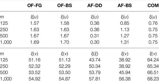
TABLE 7. Comparison of the percentage error of the velocity ξ(u) and viscosity ξ(ν) compared to the analytical solution of the Papanastasiou model (Eq. 8) and (Eq. 6) for the different regularization parameters m. All simulations were run for refinement L2 and constant velocity inlet cv.

TABLE 8

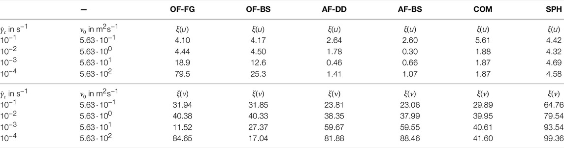
TABLE 8. Comparison of the percentage error of the velocity ξ(u) and viscosity ξ(ν) compared to the analytical solution of the bi-viscous model (Eq. 8) for the different regularization parameters (critical shear rate ${\dot{\gamma }}_c$ and critical kinematic viscosity ν₀, respectively). All simulations were run for refinement L2 and constant pressure drop cp.

3.2.2 Papanastasiou Model

In addition to the bi-viscous model, the Papanastasiou model was used in this study. This was newly implemented in Ansys Fluent and OpenFOAM, since it is not included in the standard version. The deviations of the velocity profile from the analytical solution ξ(u) is given in Table 7 as well as the viscosity deviations ξ(ν). In addition, the OpenFOAM solution (OF-FG) is shown in Supplementary Figure S7 for the velocity profiles.

Only very small differences are observed for the velocity profiles compared to the analytical solution. The results are also very similar to the bi-viscous simulations. Again, a clear tendency of increasing error with increasing regularization parameter, in this case m, is observed for both OpenFOAM versions, which give again very similar results. In contrast to the bi-viscous model, the error is also rising with Ansys Fluent (BS) with increasing m. For Ansys Fluent (DD), the reversed tendency is found again. Also the nearly constant differences in the COMSOL results.

For the determination of the viscosities, again significantly higher errors are found. The percentage error of the viscosity profiles compared to the analytical solution ξ(ν) is given in Table 7. Also, the viscosity profiles from the OpenFOAM (OF-FG) solution are shown as example in supplementary material in Supplementary Figure S8. Most software packages show a deviation of 50%. Only with Ansys Fluent (BS) lower errors are found for some simulations. The results of COMSOL are slightly higher at this point with ξ(ν) > 60%. All the software packages show an increase in the error with increasing regularization parameter m. It should be noted that the results of the OpenFOAM versions is again very comparable, while Ansys Fluent versions give different results.

The reason of those errors can be found near the regularization area. Again, the results on the pipe wall correspond very well to the analytical solution. In contrast to the bi-viscous model, however, the plug flow is not achieved so clearly. The higher the m-value, the smaller the plug flow region. The largest errors occur in the transition zone to the plug flow. Due to the latter, the errors ξ(ν) become so high.

In summary, the effect of regularization on the velocity is generally very small. In both models, the error of the velocity increases for both OpenFOAM version. For Ansys Fluent, no generally valid statement can be made. COMSOL shows in both cases nearly no dependency on the regularization parameters.

In contrast, the viscosity is partly better represented by the bi-viscous model, mainly because the plug flow is better developed. An exact resolution of the steep transition from the shear zone to the plug-flow zone is not possible with any of the models. A reliable evaluation of the viscosity is therefore not completely possible with the software packages mentioned above. One of the main reasons would be the quality of the mesh used in this work, which is not enough refined in the transition zone. Therefore, the general error given in this paper increases. However, if only the flow behavior in terms of velocity is relevant, the system can be modeled well.

TABLE 9

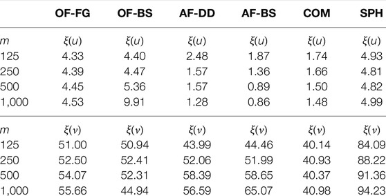
TABLE 9. Comparison of the percentage error of the velocity ξ(u) and viscosity ξ(ν) compared to the analytical solution of the Papanastasiou model (Eq. 6) for the different regularization parameters m. All simulations were run for refinement L2 and constant pressure drop cp.

FIGURE 1

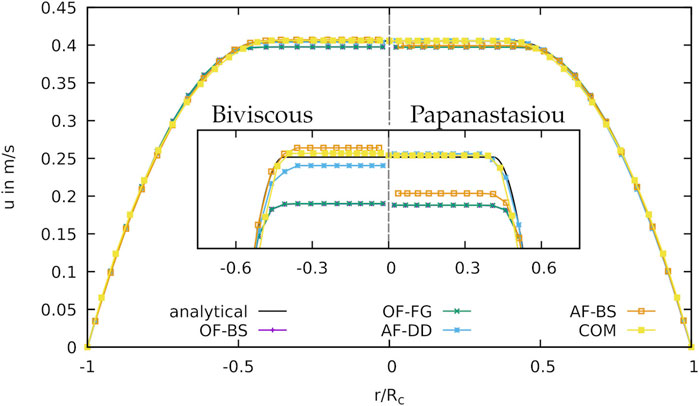
FIGURE 1. Comparison of the velocity-profiles for the different software packages with the cv boundary condition. The regularization with the bi-viscous model is shown on the left side, and the Bingham-Papanastasiou model is shown on the right. The plug-flow region is also shown enlarged for u = 0.39−0.41 m s⁻¹.

FIGURE 2

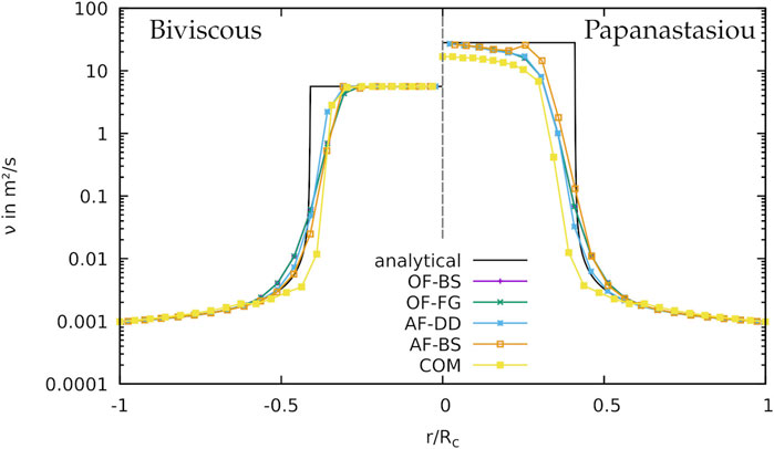
FIGURE 2. Comparison of the viscosity-profiles for the different software packages with the cv boundary condition. The regularization with the bi-viscous model is shown on the left side, and the Bingham-Papanastasiou model is shown on the right.

FIGURE 3

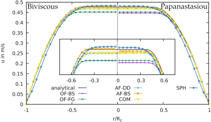
FIGURE 3. Comparison of the velocity-profiles for the different software packages with the cp boundary condition. The regularization with the bi-viscous model is shown on the left side, and the Bingham-Papanastasiou model is shown on the right. The plug-flow region is also shown enlarged for u = 0.42−0.5 m s⁻¹.

FIGURE 4

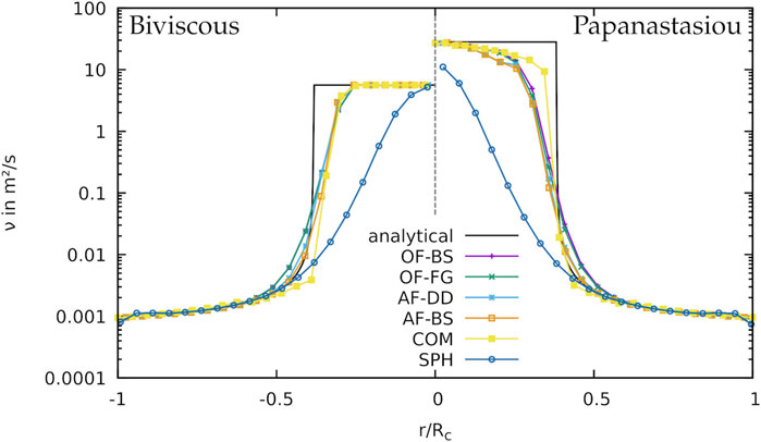
FIGURE 4. Comparison of the viscosity-profiles for the different software packages with the cp boundary condition. The regularization with the bi-viscous model is shown on the left side, and the Bingham-Papanastasiou model is shown on the right.

TABLE 10

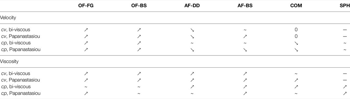
TABLE 10. Dependence of the deviation of the velocity and viscosity profiles from the analytical solution with rising regularization parameter ${\dot{\gamma }}_c$ or m for bi-viscous model or Papanastasiou model, respectively. The trend can either be rising ↗, falling ↘, undetermined ∼ or nearly constant 0. The case of missing data is marked with.

3.3 Regularization With Constant Pressure Drop Boundary Condition

In this section, the investigations on regularization of both models explained in Section 2.2.3 are reported for the constant pressure drop (cp) boundary condition. As in Section 3.2, only refinement level L2 will be used.

3.3.1 Bi-Viscous Model

First of all, the velocity profiles will be discussed. The deviations from the analytical solution are shown in Table 8. It becomes clear that the deviation are usually significantly above the comparable simulations in the cv case. Only for the cases ${\dot{\gamma }}_c=$1 × 10^–2 s⁻¹ and 1 × 10^–3 s⁻¹ a smaller deviation is found with Ansys Fluent (AF-BS) compared to cv. Moreover, the results between the two OpenFOAM versions are no longer well comparable, especially in the case of high regularization parameters. The tendency of increasing deviations with increasing regularization parameters is clearly visible similar to the cv case.

Additionally, the results of the different Ansys Fluent versions are not the same. In this case, no tendency can be found between the deviations and the regularization parameter. COMSOL shows a larger deviation only for ${\dot{\gamma }}_c=$1 × 10^–1 s⁻¹. For higher ${\dot{\gamma }}_c$ the error value is almost constant. Also SPH simulations show no noticeable dependence on the regularization parameter.

The viscosity shows a clear deviation from the analytical solution in all simulations in a similar order of magnitude as in the cv case, Table 8. The tendency of increasing deviations with increasing regularization parameter can be demonstrated for Ansys Fluent, COMSOL and HOOMD-blue.sph, but not for OpenFOAM. For the latter, the termination criterion of 1 × 10^–8 for pressure and velocity could not be reached. The simulation remained unstable.

3.3.2 Papanastasiou Model

With the Papanastasiou model, in some cases considerably better results could be found for the velocity profiles, Table 9. The dependence of the deviations on the regularization parameter are small in all simulations performed. Furthermore, the OpenFOAM versions show the tendency of increasing deviations with increasing m, whereas the Ansys Fluent versions and COMSOL show the opposite tendency. In the case of SPH, no clear dependence can be found. Compared to the cv case, the deviations are slightly higher with the constant pressure drop boundary condition.

For the viscosity profiles, this trend is also visible for OpenFOAM (OF-FG), Ansys Fluent (AF-BS) and HOOMD-blue.sph, Table 9. OF-BS, AF-DD and COMSOL, on the other hand, do not show a clear dependence on m. The deviations are similar to those in the cv case.

3.4 Comparison of Software Packages

In this section, the individual software packages are compared with each other. In the case of constant velocity boundary conditions, very good results are obtained for all simulations. The deviations of the velocity profile from the analytical solution are small with each of the software packages as shown in Figure 1. The best results in the plug-flow area are achieved with COMSOL. The influence of the regularization model is of minor importance for the determination of the velocity profile.

Strong gradients in the viscosity at the transition from shear zone to plug-flow zone, on the other hand, cannot be completely resolved by any of the software packages, Figure 2. This would require additional refinement of the mesh at the transition zone. The plug flow is in case of the bi-viscous model clearly visible, while no clearly constant viscosity is reached with the Papanastasiou model.

The fluctuations in the case of a constant pressure drop boundary condition cp, on the other hand, are much stronger. In contrast to the cv case, these fluctuations are also visible in the velocity profiles shown in Figure 3. Neither with the bi-viscous model nor with the Papanastasiou model the analytical solution can be determined very precisely. The maximum velocity is slightly underestimated by most software packages except HOOMD-blue.sph. Also the width of the plug flow varies slightly between simulations. The mesh-free SPH method gives similar good results as the mesh-based methods concerning the velocity.

The viscosity profiles can be well resolved by all software packages near the tube wall and are comparable, Figure 4. A constant viscosity in the plug flow can be achieved with the bi-viscous regularization model, but hardly with the Papanastasiou model. Here, the transition zone is also the most difficult to represent. With HOOMD-blue.sph, significant deviations in viscosity from the analytical solution become apparent in some cases. Interestingly, as described above, these have only a very small influence on the velocity profiles. The mesh-based methods give here better results.

As described in the previous sections, different trends for the dependence of the errors on the regularization parameter are found for the different software packages. These are summarized in Table 10 for the velocity and viscosity profiles.

In general, OpenFOAM on the one hand is found to have an increasing error with increasing regularization parameter regardless of the regularization model or boundary conditions. Ansys Fluent and COMSOL, on the other hand, often show the opposite trend or no trend at all. For viscosity, the error increases with increasing regularization parameter in all software packages or shows no clear trend.

4 Conclusion

In this study, a detailed comparison was presented for the simulation of yield-stress fluids using different software packages and numerical methods including commercial and open-source tools. The FEM and FVM as typical grid-based methods are compared with the meshless SPH. For the non-Newtonian fluid, a classical Bingham fluid was used, which was regularized with two different methods, namely the bi-viscous model and the Papanastasiou model.

In general, it can be stated that the type of regularization has only a minor influence on the solution, especially on the velocity. Interestingly, both OpenFOAM versions show a trend of rising errors with rising regularization parameter ${\dot{\gamma }}_c$ and m in velocity and viscosity in most of the cases. In contrast Ansys Fluent (AF-DD) shows the opposite trend for the velocity in most of the cases. In the Ansys Fluent version (AF-BS) no clear tendency can be observed in this case. COMSOL shows no or only a very small dependence on the regularization parameters.

For viscosity, very well comparable values are generally found directly at the tube walls. In the area of the transition from shear zone to plug flow, however, significant errors are observed. The larger the gradients become, the more significant the errors become. The authors conclude that grid refinement at the tube walls is of less importance than refinement in the transition zone. However, the exact position of the transition is usually not known for a flow in an experimental setup. A grid refinement is thus hardly possible at this point. Overall, it is shown that the influence of viscosity on the velocity profile tends to be small. An estimation of the flow velocities is thus possible without problems with all software packages, regardless if mesh-based or not. Even for simple flow geometries such as a laminar flow in a pipe, the viscosity in the regularization region should be used with great caution.

All software packages are able to determine the velocities with high accuracy. However, a strong dependence on the boundary conditions is observed. For a constant inlet velocity (cv), the grid-based methods produce the best results. In the case of a given pressure drop (cp), significant deviations from the analytical solution are found with all software packages.

In the first case, only small deviations of the velocity in the range of 1% and less are found. The most accurate results were achieved with Ansys Fluent and COMSOL. The results from OpenFOAM are only slightly higher. With respect to viscosity, no exact tendency can be found, since all software packages show very significant errors. The same applies to the cp simulations. As with the cv simulations, the errors for the viscosity are in the range of 50%. The SPH software produces the largest error in viscosity due to the plug flow region not being reached for bi-viscous and Papanastasiou model.

In summary, none of the software solutions is capable of achieving very good results without restrictions, especially with regard to viscosity. However, the flow behavior in the form of velocity is well represented by every method. Thus especially the determination of the viscosity strongly depends on how well the grid is refined in the area of large viscosity gradients.

Data Availability Statement

The original contributions presented in the study are included in the article/Supplementary Material, further inquiries can be directed to the corresponding authors.

Author Contributions

First draft and concept was written by MH and RS. Also MH, SF, DJ, ME, RS, DI, and NK have contributed to the concept of the paper. Simulations were done by MH, SF, DJ, ME, DI, and DR. Postprocessing of Data and formatting were done by MH, SF, DJ, RS, DR, and ME. PI of the projects are DL, CS, VM, TS, HS, and RS. All authors contributed to manuscript revision and approved the submitted version.

Funding

Gefördert durch die Deutsche Forschungsgemeinschaft (DFG), Projektnummer 387095311, 387065607, 387152355, 387066140, 387096404, 387153567, 451942209, funded by the Deutsche Forschungsgemeinschaft (DFG, German Research Foundation), Projektnummer 387095311, 387065607, 387152355, 387066140, 387096404, 387153567, 451942209.

Conflict of Interest

The authors declare that the research was conducted in the absence of any commercial or financial relationships that could be construed as a potential conflict of interest.

Publisher’s Note

All claims expressed in this article are solely those of the authors and do not necessarily represent those of their affiliated organizations, or those of the publisher, the editors and the reviewers. Any product that may be evaluated in this article, or claim that may be made by its manufacturer, is not guaranteed or endorsed by the publisher.

Supplementary Material

The Supplementary Material for this article can be found online at: https://www.frontiersin.org/articles/10.3389/fmats.2022.874144/full#supplementary-material

Footnotes

¹https://www.ansys.com/products/fluids/ansys-fluent.

²www.openfoam.com and www.openfoam.org.

References

Alfi, M., Benarjee, N., Feys, D., and Park, J. (2013). “Simulation of Formwork Filling by Cement Fluid: the Effect of the Formwork Structure on Yield-Stress Fluid,” in The Proceedings of 2013 COMSOL Conference in Boston, Boston.

Google Scholar

Anderson, J. A., Lorenz, C. D., and Travesset, A. (2008). General Purpose Molecular Dynamics Simulations Fully Implemented on Graphics Processing Units. J. Comput. Phys. 227, 5342–5359. doi:10.1016/j.jcp.2008.01.047

CrossRef Full Text | Google Scholar

Auernhammer, G., Fataei, S., Haustein, M. A., Patel, H. P., Schwarze, R., Secrieru, E., et al. (2020). Transparent Model concrete with Tunable Rheology for Investigating Flow and Particle-Migration during Transport in Pipes. Mater. Des. 193, 108673. doi:10.1016/j.matdes.2020.108673

CrossRef Full Text | Google Scholar

Bird, R. B., Stewart, W. E., and Lightfoot, E. N. (2002). Transport Phenomena. 2nd, wiley international ed edn. New York: John Wiley & Sons.

Google Scholar

Choi, M. S., Kim, Y. J., and Kim, J. K. (2014). Prediction of concrete Pumping Using Various Rheological Models. Int. J. Concr Struct. Mater. 8, 269–278. doi:10.1007/s40069-014-0084-1

CrossRef Full Text | Google Scholar

COMSOL (2019). CFD Module User’s Guide, 5, 5. Comsol Inc.

Google Scholar

De Schutter, G., and Feys, D. (2016). Pumping of Fresh concrete: Insights and Challenges. RILEM Tech. Lett. 1, 76. doi:10.21809/rilemtechlett.2016.15

CrossRef Full Text | Google Scholar

Dean, E. J., Glowinski, R., and Guidoboni, G. (2007). On the Numerical Simulation of bingham Visco-Plastic Flow: Old and New Results. J. Non-Newtonian Fluid Mech. 142, 36–62. doi:10.1016/j.jnnfm.2006.09.002

CrossRef Full Text | Google Scholar

Fataei, S., Secrieru, E., and Mechtcherine, V. (2020). Experimental Insights into concrete Flow-Regimes Subject to Shear-Induced Particle Migration (SIPM) during Pumping. Materials 13, 1233. doi:10.3390/ma13051233

PubMed Abstract | CrossRef Full Text | Google Scholar

Frigaard, I. A., and Nouar, C. (2005). On the Usage of Viscosity Regularisation Methods for Visco-Plastic Fluid Flow Computation. J. Non-Newtonian Fluid Mech. 127, 1–26. doi:10.1016/j.jnnfm.2005.01.003

CrossRef Full Text | Google Scholar

Gálvez-Moreno, D., Feys, D., and Riding, K. (2019). Characterization of Air Dissolution and Reappearance under Pressure in Cement Pastes by Means of Rheology. Front. Mater. 6, 73. doi:10.3389/fmats.2019.00073

CrossRef Full Text | Google Scholar

Geuzaine, C., and Remacle, J.-F. (2009). Gmsh: A 3-D Finite Element Mesh Generator with Built-In Pre- and post-processing Facilities. Int. J. Numer. Meth. Engng. 79, 1309–1331. doi:10.1002/nme.2579

CrossRef Full Text | Google Scholar

Giesekus, H. (1994). Phänomenologische Rheologie. Berlin, Heidelberg: Springer Berlin Heidelberg.

Google Scholar

Gingold, R. A., and Monaghan, J. J. (1977). Smoothed Particle Hydrodynamics: Theory and Application to Non-spherical Stars. Monthly Notices R. Astronomical Soc. 181, 375–389. doi:10.1093/mnras/181.3.375

CrossRef Full Text | Google Scholar

Glaser, J., Nguyen, T. D., Anderson, J. A., Lui, P., Spiga, F., Morse, D. C., et al. (2015). Strong Scaling of General-Purpose Molecular Dynamics Simulations on GPUs. Comput. Phys. Commun. 192, 97–107. doi:10.1016/j.cpc.2015.02.028

CrossRef Full Text | Google Scholar

Haustein, M. A., Kluwe, M. N., and Schwarze, R. (2020). Experimental Investigation of the Pumping of a Model-concrete through Pipes. Materials 13, 1161. doi:10.3390/ma13051161

PubMed Abstract | CrossRef Full Text | Google Scholar

Jacobsen, S., Mork, J. H., Lee, S. F., and Haugan, L. (2009). Pumping of concrete and Mortar-State of the Art. COIN Project Report 5.

Google Scholar

Jeyaraj, J. A. (2018). Numerical Modeling of concrete Flow in Drilled Shaft. PhD Thesis. University of South Florida.

Google Scholar

Jop, P., Forterre, Y., and Pouliquen, O. (2006). A Constitutive Law for Dense Granular Flows. Nature 441, 727–730. doi:10.1038/nature04801

PubMed Abstract | CrossRef Full Text | Google Scholar

Khan, N. A., Sultan, F., and Alshomrani, A. S. (2020). Binary Chemical Reaction with Activation Energy in Radiative Rotating Disk Flow of bingham Plastic Fluid. Heat Transfer 49, 1314–1337. doi:10.1002/htj.21663

CrossRef Full Text | Google Scholar

Kijanski, N., Krach, D., and Steeb, H. (2020). An SPH Approach for Non-spherical Particles Immersed in Newtonian Fluids. Materials (Basel) 13 , 1–19. doi:10.3390/ma13102324

PubMed Abstract | CrossRef Full Text | Google Scholar

Li, Y., Hao, J., Jin, C., Wang, Z., and Liu, J. (2021). Simulation of the Flowability of Fresh concrete by Discrete Element Method. Front. Mater. 7, 487. doi:10.3389/fmats.2020.603154

CrossRef Full Text | Google Scholar

Lipscomb, G. G., and Denn, M. M. (1984). Flow of bingham Fluids in Complex Geometries. J. Non-Newtonian Fluid Mech. 14, 337–346. doi:10.1016/0377-0257(84)80052-X

CrossRef Full Text | Google Scholar

Lucy, L. B. (1977). A Numerical Approach to the Testing of the Fission Hypothesis. Astronomical J. 82, 1013–1024. doi:10.1086/112164

CrossRef Full Text | Google Scholar

Mandal, S., Turek, S., Schwarze, R., Haustein, M., Ouazzi, A., and Gladky, A. (2018). Numerical Benchmarking of Granular Flow with Shear Dependent Incompressible Flow Models. J. Non-Newtonian Fluid Mech. 262, 92–106. doi:10.1016/j.jnnfm.2018.03.015

CrossRef Full Text | Google Scholar

Mechtcherine, V., Khayat, K. H., and Secrieru, E. (2020). Rheology and Processing of Construction Materials: RheoCon2 & SCC9, Vol. 23 of RILEM Bookseries. Springer International Publishing.

Google Scholar

Mehmood, A., Khan, W. A., Mahmood, R., and Rehman, K. U. (2020). Finite Element Analysis on Bingham-Papanastasiou Viscoplastic Flow in a Channel with Circular/Square Obstacles: A Comparative Benchmarking. Processes 8, 779. doi:10.3390/pr8070779

CrossRef Full Text | Google Scholar

Mitsoulis, E., and Zisis, T. (2001). Flow of bingham Plastics in a Lid-Driven Square Cavity. J. Non-newtonian Fluid Mech. 101, 173–180. doi:10.1016/s0377-0257(01)00147-1

CrossRef Full Text | Google Scholar

Mitsoulis, E. (2007). “Flows of Viscoplastic Materials: Models and Computations,” in Rheology Reviews (London: British Society of Rheology), 135–178.

Google Scholar

O’Donovan, E., and Tanner, R. (1984). Numerical Study of the bingham Squeeze Film Problem. J. Non-Newtonian Fluid Mech. 15, 75–83. doi:10.1016/0377-0257(84)80029-4

CrossRef Full Text | Google Scholar

Osorno, M., Schirwon, M., Kijanski, N., Sivanesapillai, R., Steeb, H., and Göddeke, D. (2021). A Cross-Platform, High-Performance SPH Toolkit for Image-Based Flow Simulations on the Pore Scale of Porous media. Comput. Phys. Commun. 267, 108059. doi:10.1016/j.cpc.2021.108059

CrossRef Full Text | Google Scholar

Papanastasiou, T. C. (1987). Flows of Materials with Yield. J. Rheology 31, 385–404. doi:10.1122/1.549926

CrossRef Full Text | Google Scholar

Park, C. K., Noh, M. H., and Park, T. H. (2005). Rheological Properties of Cementitious Materials Containing mineral Admixtures. Cement Concrete Res. 35, 842–849. doi:10.1016/j.cemconres.2004.11.002

CrossRef Full Text | Google Scholar

Pierre, A., Weger, D., Perrot, A., and Lowke, D. (2020a). “2D Numerical Modelling of Particle-Bed 3D Printing by Selective Paste Intrusion,” in Second RILEM International Conference on Concrete and Digital Fabrication. DC 2020. RILEM Bookseries. Editors F. Bos, S. Lucas, R. Wolfs, T. Salet (Cham: Springer), 28. doi:10.1007/978-3-030-49916-7_35

CrossRef Full Text | Google Scholar

Pierre, A., Weger, D., Perrot, A., and Lowke, D. (2020b). Additive Manufacturing of Cementitious Materials by Selective Paste Intrusion: Numerical Modeling of the Flow Using a 2D Axisymmetric Phase Field Method. Materials (Basel) 13, 1–15. doi:10.3390/ma13215024

PubMed Abstract | CrossRef Full Text | Google Scholar

N. Roussel, and A. Gram (Editors) (2014). Simulation of Fresh Concrete Flow: State-Of-The Art Report of the RILEM Technical Committee, 222-SCF, Vol. 15 of RILEM State-Of-The-Art Reports (Dordrecht: Springer Netherlands).

Google Scholar

Schaeffer, D. G. (1987). Instability in the Evolution Equations Describing Incompressible Granular Flow. J. Differential Equations 66, 19–50. doi:10.1016/0022-0396(87)90038-6

CrossRef Full Text | Google Scholar

Secrieru, E., Khodor, J., Schröfl, C., and Mechtcherine, V. (2018). Formation of Lubricating Layer and Flow Type during Pumping of Cement-Based Materials. Construction Building Mater. 178, 507–517. doi:10.1016/j.conbuildmat.2018.05.118

CrossRef Full Text | Google Scholar

Spangenberg, J., Roussel, N., Hattel, J. H., Stang, H., Skocek, J., and Geiker, M. R. (2012). Flow Induced Particle Migration in Fresh concrete: Theoretical Frame, Numerical Simulations and Experimental Results on Model Fluids. Cement Concrete Res. 42, 633–641. doi:10.1016/j.cemconres.2012.01.007

CrossRef Full Text | Google Scholar

Sultan, F., Khan, N. A., and Afridi, M. I. (2020). Investigation of Biological Mechanisms during Flow of nano-Bingham-Papanastasiou Fluid through a Diseased Curved Artery. Proc. Inst. Mech. Eng. N: J. Nanomater. Nanoengineering Nanosystems 234, 69–81. doi:10.1177/2397791420911265

CrossRef Full Text | Google Scholar

Talon, L., Auradou, H., and Hansen, A. (2014). Effective Rheology of bingham Fluids in a Rough Channel. Front. Phys. 2, 24. doi:10.3389/fphy.2014.00024

CrossRef Full Text | Google Scholar

Toutou, Z., and Roussel, N. (2007). Multi Scale Experimental Study of concrete Rheology: From Water Scale to Gravel Scale. Mater. Struct. 39, 189–199. doi:10.1617/s11527-005-9047-y

CrossRef Full Text | Google Scholar

UDF (2006). FLUENT 6.3 UDF Manual. ANSYS Inc.

Google Scholar

Wu, D., Fall, M., and Cai, S. J. (2013). Coupling Temperature, Cement Hydration and Rheological Behaviour of Fresh Cemented Paste Backfill. Minerals Eng. 42, 76–87. doi:10.1016/j.mineng.2012.11.011

CrossRef Full Text | Google Scholar