Full-Scale Simulation of the Fluid–Particle Interaction Under Magnetic Field Based on IIM–IBM–LBM Coupling Method

Introduction

Fluid–particle two-phase flows under a magnetic field can be usually found in nature and engineering applications, ranging from mineral screening (Ku et al., 2015), microfluidic control systems (Cao et al., 2014), magnetorheological fluid (Climent et al., 2004), and other chemical and biological applications. For the modeling of such flows, the two most important issues are to calculate the interaction forces between the particles and fluid/magnetic fields accurately and efficiently.

Fluid–particle interaction is one of the research hotspots in the computational fluid community. The existing models for fluid–particle interaction can fall into two categories: the Eulerian–Eulerian models and the Eulerian–Lagrangian models (Chiesa et al., 2005; Patel et al., 2017). The Eulerian–Eulerian models can capture the collective behavior of particles. However, it needs complex constitutive equations, and it is difficult to predict the details of the flow. Alternatively, the Eulerian–Lagrangian models easily obtain the detailed flowing behavior around the particles. The Eulerian–Lagrangian models can also be classified into two types: the point source model and the full-scale model (Luo et al., 2007; Hu et al., 2018). For the point source model, the empirical drag force formula is utilized to compute the fluid-particle interaction force. However, the point model i lacks enough accuracy for cases with dense or large-sized particles. For full-scale simulation, the fluid is governed by the Navier–Stokes equations, and the particle motion is solved by the Newtonian laws. The interaction force between the fluid and particle is determined by the no-slip condition. From this point of view, the full-scale model is most suitable for the study of flow mechanisms. Within the framework of full-scale models, the fixed mesh methods, which do not require time-consuming mesh generation, have received considerable attention in recent years. Unlike the body-fitted mesh methods, the governing equations of the fluid field are discretized on a fixed mesh, and the boundary is tracked by a set of Lagrangian points or captured by an implicit function. As a result, the computational efficiency is greatly improved. Kang et al. applied the distributed Lagrange multiplier/fictitious domain method to solve flows with suspended paramagnetic particles, in which the no-slip boundary condition on the particle boundary is implemented by Lagrange multipliers (Kang et al., 2008). Kang and Suh proposed the one-stage smoothed profile method for simulation of flows with suspended paramagnetic particles, in which the sigmoid function was used to construct body force by ensuring the rigidity of particles (Kang and Suh, 2011a). Kim and Park presented a level-set method for the analysis of magnetic particle dynamics on a fixed mesh (Kim and Park, 2010). Ke et al. introduced an IBM to simulate the behavior of magnetic particles in a fluid with an external magnetic field (Ke et al., 2017). These works show the effectiveness of fixed mesh methods in handling the fluid–particle interaction under a magnetic field.

In terms of calculation of magnetic force, the calculation models can also be divided into the point–dipole model and the force integration model. For example, Sand et al. developed a point–dipole model to simulate the magnetic particle suspension flow in which the single particle attraction force towards the magnetic pole was computed by a simple Kelvin force formula, and the interaction force between two nearby particles was computed by a magnetic dipole model (Sand et al., 2016). Like the point source model for fluid–particle interaction, the point–dipole model for particle–magnetic field interaction also suffers from inaccurate force estimation in nondilute flow or particle shape-dependent conditions. To this end, some work based on the force integration model has been done. In these models, the governing equation of the magnetic field in the multimedia zone was solved firstly. Then, the magnetic force acting on the particle can be obtained by integrating the force density. The magnetic force density can be calculated by the Helmholtz force density (Kang et al., 2008) or the virtual air gap scheme (Kang and Suh, 2011b). It should be pointed out that the fluid–particle interface is smeared out over several mesh cells in these above-the-force integration models. However, the magnetic stress force at the interface is treated as the continuous smoothed form, which will cause the loss of numerical accuracy.

In this paper, we develop a fully resolved simulation method for the fluid–particle interaction under a magnetic field. The LBM, which is a simple and efficient flow field solver, is adopted. The fluid–particle interaction is handled by the momentum-exchange-based IBM. More importantly, we give a Maxwell stress integration method to calculate the magnetic force based on the IIM with a finite difference scheme. According to the normal and tangential jump conditions of magnetic scalar potential along the medium interface, the discretized difference scheme is modified to ensure second-order accuracy. Then, the Maxwell stress tensor at the interface can be calculated accurately. The magnetic force acting on the particle can be obtained by integrating the magnetic stress force along the interface. Several numerical examples are simulated to validate the present IIM–IBM–LBM coupling model. The numerical results indicate that the present calculated stress force values agree well with the numerical results obtained by the body-fitted mesh. The circular particle sedimentation and motion of elliptical particles in shear flow under the magnetic field are also studied.

Mathematical Model and Numerical Method

In this study, LBM is used to simulate fluid flow, IBM is used to simulate the interaction between fluid and particles, and IIM is used to calculate magnetic field. In this section, we introduce the numerical implementation procedures of LBM, IBM, and IIM.

Lattice Boltzmann Model for Incompressible Fluid Flow

Using a standard uniform Cartesian grid with lattice space $h$, the single relaxation time LB evolution equation with external force term is as follows (Chen and Doolen, 1998):

$\begin{array}{c}{f}_{\alpha }\left(x+e_{\alpha }\text{Δ}t,t+\text{Δ}t\right)-f_{\alpha }\left(x,t\right)=-\frac{1}{\tau }\left[f_{\alpha }\left(x,t\right)-f_{\alpha }^{eq}\left(x,t\right)\right]+F_{\alpha }\text{Δ}t\end{array},(1)$

where $f_{\alpha }$ is the density distribution function. The dimensionless relaxation time reads

$\begin{array}{c}\tau =\frac{\mu }{\text{Δ}t{c}_s^2}+0.5\end{array},(2)$

where $\mu$ is the coefficient of kinetic viscosity, $f_{\alpha }^{eq}$ is the equilibrium distribution function, and $F_{\alpha }$ is the external force term in discrete velocity space. Then, $f_{\alpha }^{eq}$ and $F_{\alpha }$ could be separately written as

$\begin{array}{c}{f}_{\alpha }^{eq}={\omega }_{\alpha }{\rho }_f\left[1+\frac{{\mathit{e}}_{\alpha }\cdot \mathit{u}}{c_s^2}+\frac{{\left({\mathit{e}}_{\alpha }\cdot \mathit{u}\right)}^2}{2c_s^2}-\frac{{\mathit{u}}^2}{2c_s^2}\right]\end{array},(\mathrm{3a})$

$\begin{array}{c}{F}_{\alpha }=\left(1-\frac{1}{2\tau }\right){\omega }_{\alpha }\left[\frac{{\mathit{e}}_{\alpha }-\mathit{u}}{c_s^2}+\frac{{\mathit{e}}_{\alpha }\cdot \mathit{u}}{c_s^4}{\mathit{e}}_{\alpha }\right]\cdot \mathit{f}\end{array},(\mathrm{3b})$

where $c_s=\frac{c}{\sqrt{3}}=\frac{h}{\text{Δ}t\sqrt{3}}$ is the lattice sound speed and $\mathit{f}$ is the body force. In the D2Q9 model, the discrete velocity ${\mathit{e}}_{\alpha }$ and weight coefficients separately reads

$\begin{array}{c}{\mathit{e}}_{\alpha }=\{\begin{array}{c}\left(\mathrm{0,0}\right),\alpha =0\\ c\left(cos\left[\left(\alpha -1\right)\frac{\pi }{2}\right],sin\left[\left(\alpha -1\right)\frac{\pi }{2}\right]\right),\alpha =\mathrm{1,2,3,4}\\ \sqrt{2}c\left(cos\left[\left(2\alpha -1\right)\frac{\pi }{4}\right],sin\left[\left(2\alpha -1\right)\frac{\pi }{4}\right]\right),\alpha =\mathrm{5,6,7,8}\end{array}\end{array},(\mathrm{4a})$

$\begin{array}{c}{\omega }_0=4/9,{\omega }_1={\omega }_2={\omega }_3={\omega }_4=1/9,{\omega }_5={\omega }_6={\omega }_7={\omega }_8=1/36\end{array}.(\mathrm{4b})$

The density and macrovelocity are written as

$\begin{array}{c}{\rho }_f={\displaystyle \sum }_{\alpha }{f}_{\alpha }\end{array},(\mathrm{5a})$

$\begin{array}{c}\mathit{u}=\left({\displaystyle \sum }_{\alpha }{\mathit{e}}_{\alpha }{f}_{\alpha }+\frac{1}{2}\mathit{f}\text{Δ}t\right)/\rho \end{array}.(\mathrm{5b})$

Immersed Boundary Method for the Fluid–Particle Interaction

The momentum exchange-based IBM proposed by Niu et al. (2006) is used to calculate the interaction force between fluid and solid particles. In Figure 1, the flow domain is covered with a uniform Cartesian grid, and the fluid–solid interface is divided into a series of Lagrange points ${\mathit{X}}_l$ with the arc length $\text{Δ}{S}_l$. The relation between the body force $\mathit{f}$ on the Eulerian nodes ${\mathit{x}}_i=\left(x_i,y_i\right)$ and the force density $\mathit{f}$ on the Lagrange points ${\mathit{X}}_l=\left(X_l,Y_l\right)$ is expressed as

$\begin{array}{c}\mathit{f}\left({\mathit{x}}_i,t\right)={\displaystyle \sum }_i\mathit{F}\left({\mathit{X}}_l,t\right)D\left({\mathit{x}}_i-{\mathit{X}}_l\right)\text{Δ}{S}_{\mathit{l}}\end{array},(6)$

where $D\left({\mathit{x}}_i-{\mathit{X}}_l\right)$ is the two-dimensional discrete Dirac function. In this study, the expression of $D\left({\mathit{x}}_i-{\mathit{X}}_l\right)$ proposed by Peskin (Peskin, 2002) is adopted:

$\begin{array}{c}D\left({\mathit{x}}_i-{\mathit{X}}_l\right)=\frac{1}{h^2}\delta \left(\frac{x_i-X_l}{h}\right)\delta \left(\frac{y_i-Y_l}{h}\right)\end{array},(7)$

where

$\begin{array}{c}\delta \left(r\right)=\{\begin{array}{cc}\frac{1}{4}\left(1+cos\left(\frac{\pi r}{2}\right)\right)& \left|r\right|\le 2\\ 0& \left|r\right|>2\end{array}\end{array}.(8)$

FIGURE 1

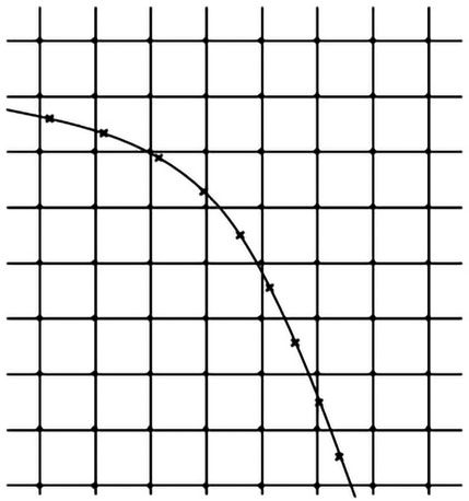
FIGURE 1. Configuration of the grids used in the IBM. Euler points (circles) represent the flow field and Lagrange points (crosses) represent the fluid–solid interface.

The calculation of the force density $\mathit{F}\left({\mathit{X}}_l,t\right)$ is the key problem in IBM, and it is usually determined by the no-slip condition on the boundary of the rigid particle. For the present momentum exchange-based IBM, the no-slip condition is implemented by the bounce-back rule. Firstly, the density distribution function $f_{\alpha }\left({\mathit{X}}_l,t\right)$ at Lagrange points is obtained by an interpolation method, i.e.,

$\begin{array}{c}{f}_{\alpha }\left({\mathit{X}}_l,t\right)={\displaystyle \sum }_{i,j}D\left({\mathit{x}}_i-{\mathit{X}}_l\right)f_{\alpha }\left({\mathit{x}}_i,t\right)h^2\end{array}.(9)$

Then, the new distribution function $f_{\alpha }^{new}\left({\mathit{X}}_l,t\right)$ could be solved according to the bounce-back rule:

$\begin{array}{c}{f}_{\alpha }^{new}\left({\mathit{X}}_l,t\right)=f_{-\alpha }\left({\mathit{X}}_l,t\right)-2{\omega }_{-\alpha }\rho \frac{e_{-\alpha }\cdot {\mathbf{U}}_B^d\left({\mathit{X}}_l,t\right)}{c_s^2}\end{array},(10)$

where ${\mathbf{U}}_B^d\left({\mathit{X}}_l,t\right)$ is the velocity at Lagrange point and $-\alpha$ is the opposite direction of $\alpha$. Next, the force density $\mathit{F}\left({\mathit{X}}_l,t\right)$ of the flow field acting on the boundary point is calculated as

$\begin{array}{c}\mathit{F}\left({\mathit{X}}_l,t\right)={\displaystyle \sum }_{\alpha }{\mathit{e}}_{\alpha }\left[f_{\alpha }^{new}\left({\mathit{X}}_l,t\right)-f_{\alpha }\left({\mathit{X}}_l,t\right)\right]\frac{h}{\text{Δ}t}\end{array}.(11)$

Furthermore, we define

$\begin{array}{c}\{\begin{array}{c}{\mathit{F}}_{pf}^{\prime }=-{\displaystyle \sum }_l\mathit{F}\left({\mathit{X}}_l,t\right)\text{Δ}{S}_l\\ {\mathit{T}}_{pf}^{\prime }=-{\displaystyle \sum }_l\left({\mathit{X}}_{\mathit{l}}-{\mathit{X}}_{\mathit{p}}\right)\times \mathit{F}\left({\mathit{X}}_l,t\right)\text{Δ}{S}_l \end{array}\end{array}.(12)$

The hydrodynamic force ${\mathit{F}}_{pf}$ and moment ${\mathit{T}}_{pf}$ acting on the solid particle can be obtained by removing the effect of internal mass

$\begin{array}{c}\{\begin{array}{c}{\mathit{F}}_{pf}={\mathit{F}}_{pf}^{\prime }+\frac{{\rho }_f}{{\rho }_p}{M}_p\frac{d{\mathit{U}}_p}{dt}\\ {\mathit{T}}_{pf}={\mathit{T}}_{pf}^{\prime }+\frac{{\rho }_f}{{\rho }_p}{I}_p\frac{d{\mathit{\omega }}_p}{dt}\end{array}\end{array},(13)$

where ${\mathit{X}}_{\mathit{p}}$ is the centroid of the solid particle, ${\rho }_p$ is the particle density, $M_p$ is the mass of particle, $I_p$ is the moment of inertia, ${\mathit{U}}_p$ is the translational velocity, and ${\mathit{\omega }}_p$ is the rotational velocity, respectively.

Immersed Interface Method for Magnetic Field Calculation

The magnetic field in the multimedia zone can be solved by the Maxwell equations with the interface conditions. As shown in Figure 2, we consider two types of methods to impose the magnetic field: one is the given external uniform magnetic field, and the other is the permanent magnetic field. The Maxwell equations without current are expressed as follows:

$\begin{array}{c}\{\begin{array}{c}\nabla \cdot \mathit{B}=0\\ \nabla \times \mathit{H}=0\end{array}\end{array},(14)$

where $\mathit{B}$ is magnetic induction and $\mathit{H}$ is magnetic field intensity. To solve the two Maxwell’s equations, the constitutive relationships between magnetic flux density and magnetic field (Eq. 15) are needed

$\begin{array}{c}\{\begin{array}{cc}\mathit{B}=\mathit{\mu }\mathit{H}& \mathrm{ }\\ \mathit{B}={\mathit{\mu }}_{\mathbf{0}}\left(\mathit{H}+\mathit{M}\right)& \left(\mathrm{for}\mathrm{permanent}\mathrm{magnet}\right)\end{array}\end{array},(15)$

where ${\mu }_0$ is permeability of vacuum, $\mu$ is relative permeability, and $\mathit{M}$ is the remanence of permanent magnet. At a current-free interface between two media, the following two continuity conditions are satisfied:

$\begin{array}{c}\{\begin{array}{c}{B}_{1\text{n}}=B_{2n}\\ H_{1\tau }=H_{2\tau }\end{array}\end{array},(16)$

where $\text{n}$ and $\tau$ are the normal and tangential directions, respectively. At the interface between permanent magnet and other media, the normal component of $\mathit{B}$ is still continuous across the interface. However, the tangential component of $\mathit{H}$ has a jump discontinuity.

$\begin{array}{c}\{\begin{array}{c}{B}_{1\text{n}}=B_{2n}\\ H_{1\tau }-H_{2\tau }=M_{2\tau }\end{array}\end{array}.(17)$

FIGURE 2

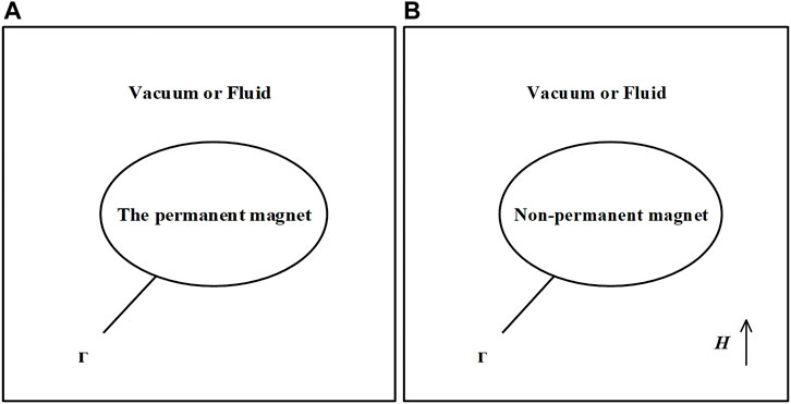
FIGURE 2. Interface problems of permanent magnetic field (A) and uniform magnetic field (B).

Due to the irrotationality condition of $\mathit{H}$ field, the scalar magnetic potential $V$ is introduced:

$\begin{array}{c}\mathit{H}=-\nabla V\end{array}.(18)$

The equations for solving the magnetic potential $V$ can be obtained:

$\begin{array}{c}\{\begin{array}{cc}\nabla \cdot \mu \left(-\nabla V\right)=0& \mathrm{ }\\ -\nabla \cdot {\mu }_0\left(\nabla V-\mathit{M}\right)=0& \left(\mathrm{for}\mathrm{permanent}\mathrm{magnet}\right)\end{array}\end{array}.(19)$

The interface conditions for $V$ could be obtained from Formula 19 as follows:

$\begin{array}{c}\{\begin{array}{c}\left[\left[\mu \nabla V\cdot \mathit{n}\right]\right]=0\\ \left[\left[\nabla V\cdot \mathit{\tau }\right]\right]=0\end{array}\left(\text{nonpermanent magnet}\right)\end{array},(20)$

$\begin{array}{c}\{\begin{array}{c}\left[\left[\nabla V\cdot \mathit{n}\right]\right]=\mathit{M}\cdot \mathit{n}\\ \left[\left[\nabla V\cdot \mathit{\tau }\right]\right]=\mathit{M}\cdot \mathit{\tau }\end{array}\left(\text{permanent magnet}\right)\end{array}.(21)$

In order to solve the magnetic field and compute magnetic force accurately, the IIM is used. The basic idea of IIM is to adopt the interface jump conditions to modify the finite difference scheme near the interface. As a result, second-order solutions can be achieved in the whole domain. A finite difference scheme for Poisson equation (Eq. 19) can be written as

$\begin{array}{c}{\displaystyle \sum }_k{\gamma }_k{V}_{i+i_k,j+j_k}=C_{ij}\end{array},(22)$

for use at the point $\left(x_i,y_j\right)$. To sum over k involves points (not more than six points selected near the interface) neighboring point $(x_i,y_j)$, so the value of each $i_k,j_k$ is set to $\left(-\mathrm{1,0,1}\right)$. The coefficients ${\gamma }_k$ and indices $i_k,j_k$ depend on $(i,j)$. The correction term $C_{ij}$ is nonzero only if the grid point is irregular. For more details, please refer to LeVeque et al. (1994).

The following formula is used to solve the magnetic field force.

$\begin{array}{c}{\mathit{F}}_m={\displaystyle \oint \mathit{n}\cdot {\mathbf{\sigma }}_{m}dS}\end{array}.(23)$

The Maxwell stress tensor is

$\begin{array}{c}{\mathbf{\sigma }}_m=-\frac{1}{2}{\text{μ}}_0{H}^2\mathit{I}+\mathit{B}\mathit{H}\end{array},(24)$

where $\mathit{I}$ is the identity operator. Moreover, the magnetic field force ${\mathit{F}}_m$ is solved by the following formula (Blūms et al., 1997):

$\begin{array}{l}{\mathit{F}}_m={\displaystyle \oint \left(-\frac{1}{2}{\mu }_0\mathit{n}\cdot H^2+\left(\mathit{n}\cdot \mathit{B}\right)\mathit{H}\right)dS},\\ \begin{array}{c}\approx {\displaystyle \sum }_l\left(-\frac{1}{2}{\mu }_0\mathit{n}\left({\mathit{X}}_{\mathit{l}}\right)\cdot H{\left({\mathit{X}}_{\mathit{l}}\right)}^2+\left(\mathit{n}\left({\mathit{X}}_{\mathit{l}}\right)\cdot \mathit{B}\left({\mathit{X}}_{\mathit{l}}\right)\right)\mathit{H}\left({\mathit{X}}_{\mathit{l}}\right)\right)\text{Δ}{S}_l\end{array},\end{array}(25)$

where $\mathit{n}$ is the normal vector. So, the magnetic field intensity at the interface needs to be determined.

Here, we introduce a six-point interpolation method to calculate from the correct side of the interface. In Figure 3, for the point P on the interface, we find the nearest point $\left(x_i,y_j\right)$ in the Cartesian grid. So, the stencil for six points is $\begin{array}{c}\left(x_{i-1},y_j\right),\left(x_i,y_j\right),\left(x_{i+1},y_j\right),\left(x_i,y_{j-1}\right),\left(x_i,y_{j+1}\right),\left(x_{i+i_0},y_{j+j_0}\right)\end{array}$, and they transform them into interface coordinates as follows. $\begin{array}{c}\left({\xi }_1,{\eta }_1\right),\left({\xi }_2,{\eta }_2\right),\left({\xi }_3,{\eta }_3\right),\left({\xi }_4,{\eta }_4\right),\left({\xi }_5,{\eta }_5\right),\left({\xi }_6,{\eta }_6\right).\end{array}$

FIGURE 3

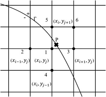
FIGURE 3. Selection of six points in the modified six-point method. Select the Euler point 1 closest to the Lagrange point (P), and the sixth point is the Euler point closest to the Lagrange point (P) except points 1 to 5.

Applying the Taylor expansion method for each point, we have

$\begin{array}{c}u\left({\xi }_k,{\eta }_k\right)=u^{\pm }+{\xi }_k{u}_{\xi }^{\pm }+{\eta }_k{u}_{\eta }^{\pm }+\frac{1}{2}{\xi }_k^2{u}_{\xi \xi }^{\pm }+{\xi }_k{\eta }_k{u}_{\xi \eta }^{\pm }+\frac{1}{2}{\eta }_k^2{u}_{\eta \eta }^{\pm }+O\left(h^3\right)\end{array}.(26)$

Ignoring the high order term $O\left(h^3\right)$, we can obtain a six-variable linear equation for.

$u^{\pm },u_{\xi }^{\pm },u_{\eta }^{\pm },u_{\xi \xi }^{\pm },u_{\xi \eta }^{\pm },u_{\eta \eta }^{\pm }$. Once $u^{\pm },u_{\xi }^{\pm },u_{\eta }^{\pm }$ are obtained, we can get $V^{\pm },H_{\xi }^{\pm },H_{\eta }^{\pm }$ at point P on the interface.

Particle Dynamics

In this study, the dynamics of particle adopts Newton’s equation of motion, and the equations controlling particle translation and rotation are as follows:

$\begin{array}{c}\{\begin{array}{c}\left(1-\frac{{\rho }_f}{{\rho }_p}\right)M_p\frac{d{\mathit{U}}_p}{dt}={\mathit{F}}_{pf}^{\prime }+{\mathit{F}}_m+{\mathit{F}}_g\\ \left(1-\frac{{\rho }_f}{{\rho }_p}\right)I_p\frac{d{\mathit{\omega }}_p}{dt}={\mathit{T}}_{pf}^{\prime }+{\mathit{T}}_m\end{array}\end{array},(27)$

$\begin{array}{c}\{\begin{array}{c}\frac{d{\mathit{X}}_p}{dt}={\mathit{U}}_p\\ \frac{d{\mathit{\theta }}_p}{dt}={\mathit{\omega }}_p\end{array}\end{array},(28)$

where ${\mathit{\theta }}_p$ is the rotation angle, ${\mathit{F}}_g$ is the gravity force, and ${\mathit{F}}_{pf}^{\prime }$ and ${\mathit{F}}_m$ are the hydrodynamics force and magnetic force acting on the particle. To avoid the numerical instability due to the low-density ratio, the following time-stepping scheme for Eq. 29 is utilized:

$\begin{array}{c}\{\begin{array}{c}{\mathit{U}}_p\left(t_{n+1}\right)=\left[b{\mathit{U}}_p\left(t_n\right)+c{\mathit{U}}_p\left(t_{n-1}\right)+\frac{\text{Δ}t\left({\mathit{F}}_{pf}^{\prime }+{\mathit{F}}_m+{\mathit{F}}_g\right)}{M_p}\right]/a\\ {\mathit{\omega }}_p\left(t_{n+1}\right)=\left[b{\mathit{\omega }}_p\left(t_n\right)+c{\mathit{\omega }}_p\left(t_{n-1}\right)+\frac{\text{Δ}t\left({\mathit{T}}_{pf}^{\prime }+{\mathit{T}}_m\right)}{I_p}\right]/a\end{array}\end{array},(29)$

where $a=3\left({\rho }_p/{\rho }_f-1\right)$, $b=2a-\left({\rho }_p/{\rho }_f-1\right)$, and $c=\left({\rho }_p/{\rho }_f-1\right)-a$ (Hu et al., 2015). We could easily obtain the center of mass ${\mathit{X}}_p\left(t_{n+1}\right)$, the rotation angle ${\mathit{\theta }}_p\left(t_{n+1}\right)$, the translational velocity ${\mathit{U}}_p\left(t_{n+1}\right)$, and the rotational velocity ${\mathit{\omega }}_p\left(t_{n+1}\right)$ of particle at time $t_{n+1}=t_n+\text{Δ}t$.

$\begin{array}{c}\{\begin{array}{c}{\mathit{X}}_p\left(t_{n+1}\right)={\mathit{X}}_p\left(t_n\right)+\frac{1}{2}\left[{\mathit{U}}_p\left(t_{n+1}\right)+{\mathit{U}}_p\left(t_n\right)\right]\text{Δ}t\\ {\mathit{\theta }}_p\left(t_{n+1}\right)={\mathit{\theta }}_p\left(t_n\right)+\frac{1}{2}\left[{\mathit{\omega }}_p\left(t_{n+1}\right)+{\mathit{\omega }}_p\left(t_n\right)\right]\text{Δ}t\end{array}\end{array}.(30)$

Then, the velocity ${\mathbf{U}}_B^d\left({\mathit{X}}_l\right)$ at the boundary point can be written as

$\begin{array}{c}{\mathbf{U}}_B^d\left({\mathit{X}}_l\right)={\mathit{U}}_p+{\mathit{\omega }}_p\times \left({\mathit{X}}_l-{\mathit{X}}_p\right)\end{array}.(31)$

Numerical Results and Discussion

In this section, the present IIM–IBM–LBM model is used to simulate several problems with fluid–particle–magnetic interaction.

Numerical Method Validation

Particle Dynamics Verification of IB–LBM

In order to examine the accuracy of the present IB–LBM, the free settlement of a single particle is simulated, which has been used by some scholars as a benchmark problem (Glowinski et al., 2001; Hu et al., 2015). In Figure 4A, we use a fluid domain with a width of 2 cm and a height of 6 cm, where the fluid density is ${\rho }_f=1.0g/c{m}^2$. A circular particle with a diameter of 0.25 cm falls freely from the position of 1 cm and 4 cm under the effect of gravity. The particle density is set as ${\rho }_p=1.25g/c{m}^2\text{ and }1.5g/c{m}^2$, and the corresponding kinematic viscosity is $\nu =0.1c{m}^2/s\text{ and }0.01c{m}^2/s$, respectively.

FIGURE 4

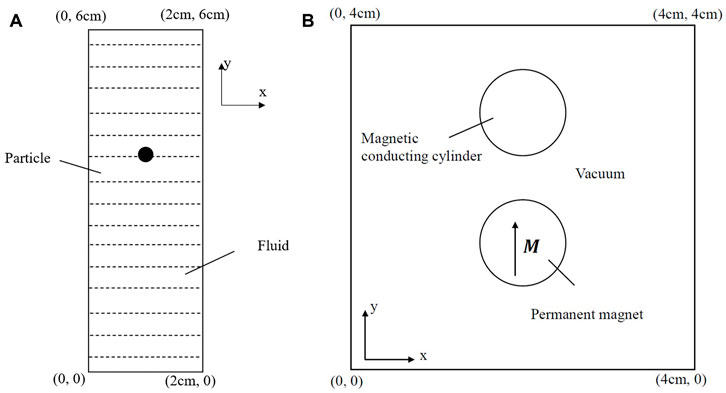
FIGURE 4. Model of free settlement of a single particle (A). Model of permanent magnet attracting magnetic conducting cylinder (B).

A $200\times 600$ grid is used for the numerical simulation. Figures 5A,B show the variations in vertical position and velocity of the particle center with time when ${\rho }_p=1.25g/c{m}^2$ and $\nu =0.1c{m}^2/s$, respectively. Obviously, the particle quickly reaches the terminal velocity, and the velocity becomes small when the particle is close to the bottom wall at about $t=0.8s$. The results are in good agreement with those of Hu et al. (Hu et al., 2015) and Glowinski et al. (Glowinski et al., 2001). Similarly, we simulate the case with ${\rho }_p=1.5g/c{m}^2$ and $\nu =0.01c{m}^2/s$. As shown in Figures 5C,D, the desired results are obtained.

FIGURE 5

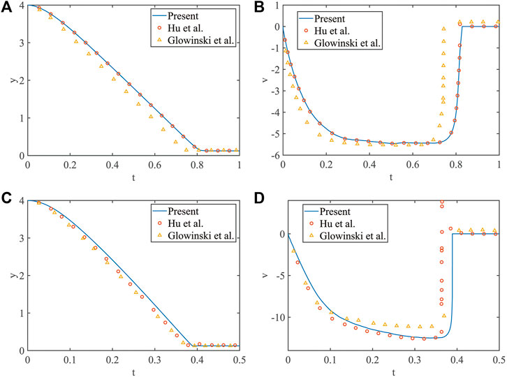
FIGURE 5. The position of the center of the particle for ${\rho }_p=1.25g/c{m}^2$, $\nu =0.1c{m}^2/s$ (A); ${\rho }_p=1.5g/c{m}^2$, $\nu =0.01c{m}^2/s$ (C), and the velocity of that for ${\rho }_p=1.25g/c{m}^2$, $\nu =0.1c{m}^2/s$ (B); ${\rho }_p=1.5g/c{m}^2$, $\nu =0.01c{m}^2/s$ (D).

Verification of Magnetic Field Calculation of IIM

To test the accuracy of IIM in terms of calculation of magnetic field, the problem of a permanent magnet attracting a magnetic conducting cylinder is studied. The results obtained are compared with those calculated by COMSOL in which the body-fitted mesh is used. As shown in Figures 4A,B, a circular permanent magnet with remanence $\mathit{M}=\left(\mathrm{0,75000}\text{A}/\text{m}\right)$ and a circular magnetic conducting object with ${\mu }_r=2.0$ are centered at (2 cm, 1.5 cm) and (2 cm, 3 cm), respectively. Both circular solids are 0.8 cm in diameter. The computational domain is a square with a side length of 4 cm.

This numerical simulation is carried out in a $400\times 400$ grid. Figure 6 displays the distribution of magnetic potential $V$, and it can be seen clearly that the jump of the magnetic field is in the normal direction across the interface. Figure 7 shows the magnetic field distribution. It could be observed that the closer the permanent magnet, the stronger the magnetic field intensity. Also, the contours of $\left|\mathbf{H}\right|$ across magnetic conducting cylinder interface have a jump. We can see that the present results agree well with those of COMSOL (Figure 7). The horizontal and vertical components of magnetic stress $f_m$ along the interface are plotted in Figure 8, and the symmetrical distribution of them can be found. The numerical results of the total magnetic force acting on the magnetic conducting cylinder are shown in Table 1. As expected, compared with the results obtained by the diffusion interface method, IIM based on the non-body–fitted grid technology can obtain the calculation accuracy similar to that of COMSOL based on the body-fitted grid technology.

FIGURE 6

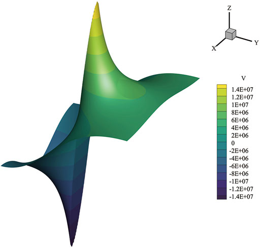
FIGURE 6. The magnetic potential $V$ of the permanent magnet attracting the particle model is obtained by the IIM method.

FIGURE 7

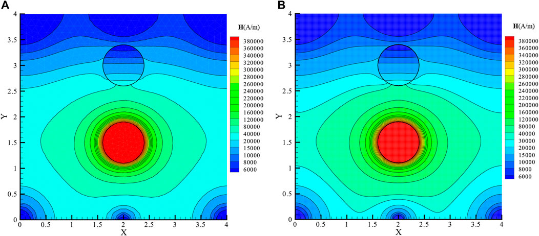
FIGURE 7. The permanent magnet attracts the magnetic field of the magnetic conducting cylinder model, which is calculated by COMSOL (A) and IIM (B).

FIGURE 8

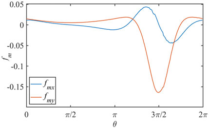
FIGURE 8. Magnetic stress $f_m$ along the interface of the circular conducting magnet.

TABLE 1

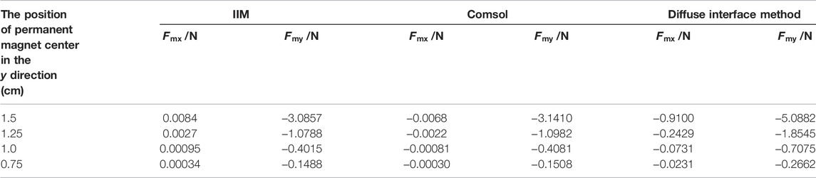
TABLE 1. The magnetic force on the magnetic conducting cylinder.

Particle Sedimentation Under Permanent Magnetic Field

The diagram of particle sedimentation under a permanent magnetic field is shown in Figure 9. The computational domain for the magnetic field is 8 cm wide and 8 cm high. The computational domain for the flow field is 2 cm wide and 6 cm high. The circular particle with ${\mu }_{rp}=2.0$ and diameter of 0.25 cm is located (4 cm, 6 cm), and the circular permanent magnet with diameter of 0.8 cm is located (4 cm, 1 cm). The remanence of the permanent magnet is $\mathit{M}=\left(\mathrm{0,75000}\text{A}/\text{m}\right)$. In this study, the relative permeability ${\mu }_{rf}$ of the flow field is set to 1.0.

FIGURE 9

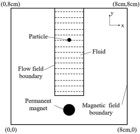
FIGURE 9. Model of particle sedimentation under the action of permanent magnet.

A $800\times 800$ grid is used for the present numerical simulation. The flow field simulation is carried out on a $200\times 600$ grid. Figure 10 shows the variations in vertical position and velocity of the particle center with time when ${\rho }_p=1.25g/c{m}^2$ and $\nu =0.1c{m}^2/s$, respectively. Due to the coexistence of magnetic force and gravity force, the particle settling velocity becomes larger compared with that without the effect of a permanent magnet. The closer the particle is to the permanent magnet, the greater the magnetic force and the faster the particle velocity. When $t=0.5s$, the acceleration effect of magnetic force on particles is dominant. Figure 11 displays the variety of magnetic stress at the particle interface at $t=0.4s, 0.5s, 0.6s$. Similarly, we also study the case with ${\rho }_p=1.5g/c{m}^2$ and $\nu =0.01c{m}^2/s$ and reached similar conclusions (as shown in Figure 12).

FIGURE 10

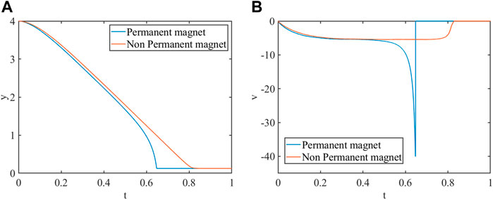
FIGURE 10. Position (A) and velocity (B) of the center of the particle for ${\rho }_p=1.25g/c{m}^2$ and $\nu =0.1c{m}^2/s$.

FIGURE 11

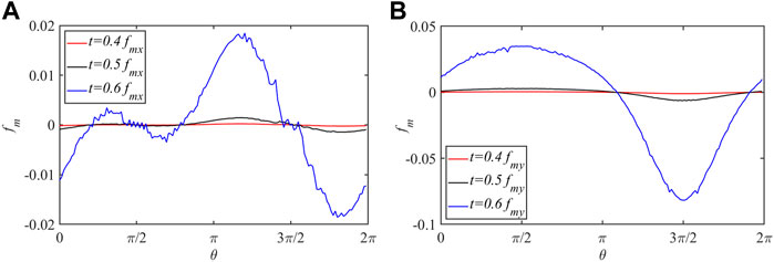
FIGURE 11. The magnetic stress $f_m$ in x-direction (A) and in y-direction (B) on the particle interface at $t=0.4s, 0.5s, 0.6s$.

FIGURE 12

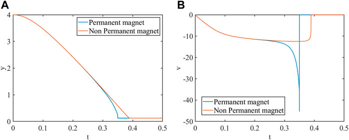
FIGURE 12. Position (A) and velocity (B) of the center of the particle for ${\rho }_p=1.5g/c{m}^2$ and $\nu =0.01c{m}^2/s$.

Shear Viscosity of Suspension Containing Elliptical Particles Under the Magnetic Field

It should be pointed out that the point–dipole model is suitable for spherical-like particles. We also consider an ellipsoidal particle immersed in the two-dimensional shear flows, as shown in Figure 13. In order to verify the reliability of the numerical method, we calculate an example of an elliptic particle rotating in a simple shear flow when Reynolds number $Re=1$ and the ratio of major axis to minor axis of ellipse $\alpha =2$. The curve of angular velocity changing with angular rotation is obtained in Figure 14 and compared with the exact solution calculated by Jeffery (Jeffery, 1922). The simulation results of this paper agree well with Jeffery’s exact solution.

FIGURE 13

FIGURE 13. An ellipsoidal particle in the two-dimensional shear flows under uniform magnetic field.

FIGURE 14

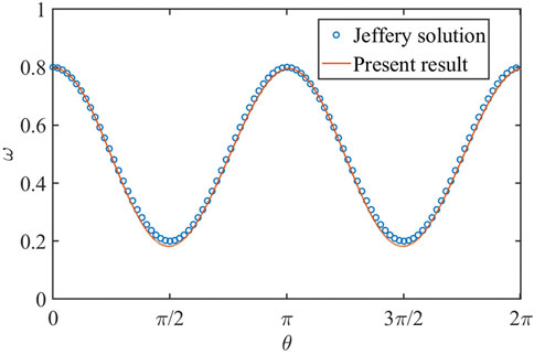
FIGURE 14. Comparison of Jeffery solution (Jeffery, 1922) and the present simulation result.

The relation between angular velocity $\omega$ and angle $\theta$ of the elliptic particle in shear flow obtained by Jeffery (Jeffery, 1922) is as follows:

$\begin{array}{c}\omega =\frac{G}{m^2+n^2}\left(m^2{\cos }^2\theta +n^2{\sin }^2\theta \right)\end{array},(32)$

where the fluid shear rate $G=2U_0/h_f$ and $m,n$ are the length of long and short half axle.

Then, we study the shear viscosity of suspension containing elliptical particles under the magnetic field. The computational domain is 2 cm long and 1 cm wide, in which the velocities of the upper and lower planes are $U_0=0.1cm/s$ and $-U_0$, respectively. The elliptical particle with length–width ratio $AR=2.0$ and relative permeability ${\mu }_{rp}=2.0$ is located at the center of the computational domain. Under an external uniform magnetic field ${\mathit{H}}_{\mathit{b}}=(0,H_0)$, the force acting on the paramagnetic ellipsoid particle is zero, but the torque is not zero.

The shear stress at the fluid node is calculated as

$\begin{array}{c}{\sigma }_{xy}=-\left(1-\frac{1}{2\tau }\right){\displaystyle \sum }_{\alpha =0}^8\left(f_{\alpha }-f_{\alpha }^{eq}\right)e_{\alpha x}{e}_{\alpha y}\end{array}.(33)$

To study the simple rheological properties of a suspension containing elliptical particles under the external magnetic field, the effective viscosity of the suspension is calculated:

$\begin{array}{c}{\nu }_e={\overline{\sigma }}_{xy}{h}_0/\left(\rho U_0\right)\end{array},(34)$

where $h_0$ is the distance between two plates and $U_0$ is the speed of the top plate. ${\overline{\sigma }}_{xy}$ is the average shear force acting on the moving plane wall (Huang et al., 2012).

A grid of $200\times 100$ is used for the calculation domain, and the left and right boundaries are subjected to the periodic boundary conditions. We set the initial deflection angle of the ellipse particle ${\theta }_e$ to $pi/4$. When the flow field becomes steady state, the effective shear viscosity ${\nu }_e$ of the suspension containing the elliptical particle under the magnetic field can be obtained. Through the present direct numerical simulation, the effective shear viscosities under different magnetic field strength ${\mathit{H}}_0$, Reynolds number $Re$, and volume fraction $\phi$ of elliptical particles in suspension are compared, as shown in Figure 15. Obviously, the effective kinematic viscosity ${\nu }_e$ increases with an increase in Reynolds number $Re$ and decreases with an increase in volume fraction $\phi$. Moreover, the effective kinematic viscosity ${\nu }_e$ increases with the increase of magnetic field strength $H_0$.

FIGURE 15

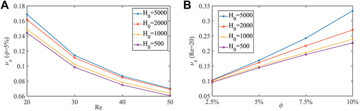
FIGURE 15. Variation of effective kinematic viscosity ${\nu }_e$ of suspension with Reynolds number in different magnetic field strength ${\text{H}}_0$ when $\phi$ is 5% (A). Variation of effective kinematic viscosity ${\nu }_e$ of suspension with volume fraction in different magnetic field strength ${\text{H}}_0$ when $Re$ is 20 (B).

Conclusion

The fluid–particle–magnetic interactions are modeled using the IIM–IBM–LBM coupling method. The fluid flow simulations are handled by the simple and efficient LBM. The particle motion and the hydrodynamics interaction between the particle and the flow field are computed by the momentum exchange-based IBM. Especially, we use the IIM to solve the magnetic field and calculate the magnetic force with the aid of the interface jump conditions. Unlike the point-source model or point dipole model, the hydrodynamics and magnetic forces acting on the particle are calculated using an integration method, in which the flow details and magnetic distribution around the particle are considered. Two numerical examples are simulated to verify the numerical accuracy of the present full-scale model. Moreover, particle sedimentation under a permanent magnetic field and shear viscosity of suspension containing elliptical particles under the magnetic field are also studied by the present model. The obtained results indicate that the present model has the potential to treat the complex fluid–particle–magnetic interactions.

Data Availability Statement

The original contributions presented in the study are included in the article/supplementary material; further inquiries can be directed to the corresponding author.

Author Contributions

All authors listed have made a substantial, direct, and intellectual contribution to the work and approved it for publication.

Funding

This work was supported by the National Natural Science Foundation of China (grant nos. 12172039, 12102228, and 11802159) and Fundamental Research Funds for the Central Universities (grant no. 2020RC201).

Conflict of Interest

The authors declare that the research was conducted in the absence of any commercial or financial relationships that could be construed as a potential conflict of interest.

Publisher’s Note

All claims expressed in this article are solely those of the authors and do not necessarily represent those of their affiliated organizations or those of the publisher, the editors, and the reviewers. Any product that may be evaluated in this article, or claim that may be made by its manufacturer, is not guaranteed or endorsed by the publisher.

References

Blūms, E., T͡Sebers, A. O., Cebers, A. O., and Maiorov, M. M. (1997). Magnetic Fluids. Berlin, Germany: Walter de Gruyter.

Google Scholar

Cao, Q., Han, X., and Li, L. (2014). Configurations and Control of Magnetic Fields for Manipulating Magnetic Particles in Microfluidic Applications: Magnet Systems and Manipulation Mechanisms. Lab. Chip 14 (15), 2762–2777. doi:10.1039/c4lc00367e

PubMed Abstract | CrossRef Full Text | Google Scholar

Chen, S., and Doolen, G. D. (1998). Lattice Boltzmann Method for Fluid Flows. Annu. Rev. Fluid Mech. 30 (1), 329–364. doi:10.1146/annurev.fluid.30.1.329

CrossRef Full Text | Google Scholar

Chiesa, M., Mathiesen, V., Melheim, J. A., and Halvorsen, B. (2005). Numerical Simulation of Particulate Flow by the Eulerian-Lagrangian and the Eulerian-Eulerian Approach with Application to a Fluidized Bed. Comput. Chem. Eng. 29 (2), 291–304. doi:10.1016/j.compchemeng.2004.09.002

CrossRef Full Text | Google Scholar

Climent, E., Maxey, M. R., and Karniadakis, G. E. (2004). Dynamics of Self-Assembled Chaining in Magnetorheological Fluids. Langmuir 20 (2), 507–513. doi:10.1021/la035540z

PubMed Abstract | CrossRef Full Text | Google Scholar

Glowinski, R., Pan, T. W., Hesla, T. I., Joseph, D. D., and Périaux, J. (2001). A Fictitious Domain Approach to the Direct Numerical Simulation of Incompressible Viscous Flow Past Moving Rigid Bodies: Application to Particulate Flow. J. Comput. Phys. 169 (2), 363–426. doi:10.1006/jcph.2000.6542

CrossRef Full Text | Google Scholar

Hu, Y., Li, D., Shu, S., and Niu, X. (2015). Modified Momentum Exchange Method for Fluid-Particle Interactions in the Lattice Boltzmann Method. Phys. Rev. E Stat. Nonlin Soft Matter Phys. 91 (3), 033301. doi:10.1103/PhysRevE.91.033301

PubMed Abstract | CrossRef Full Text | Google Scholar

Hu, Y., Li, D., Niu, X., and Shu, S. (2018). Fully Resolved Simulation of Particulate Flows with Heat Transfer by Smoothed Profile-Lattice Boltzmann Method. Int. J. Heat Mass Transf. 126, 1164–1167. doi:10.1016/j.ijheatmasstransfer.2018.05.137

CrossRef Full Text | Google Scholar

Huang, H., Yang, X., Krafczyk, M., and Lu, X.-Y. (2012). Rotation of Spheroidal Particles in Couette Flows. J. Fluid Mech. 692, 369–394. doi:10.1017/jfm.2011.519

CrossRef Full Text | Google Scholar

Jeffery, G. B. (1922). The Motion of Ellipsoidal Particles Immersed in a Viscous Fluid. Proc. R. Soc. Lond. Ser. A Contain. Pap. Math. Phys. Character 102 (715), 161–179. doi:10.1098/rspa.1922.0078

CrossRef Full Text | Google Scholar

Kang, S., and Suh, Y. K. (2011). An Immersed-Boundary Finite-Volume Method for Direct Simulation of Flows with Suspended Paramagnetic Particles. Int. J. Numer. Meth. Fluids 67 (1), 58–73. doi:10.1002/fld.2336

CrossRef Full Text | Google Scholar

Kang, S., and Suh, Y. K. (2011). Direct Simulation of Flows with Suspended Paramagnetic Particles Using One-Stage Smoothed Profile Method. J. Fluids Struct. 27 (2), 266–282. doi:10.1016/j.jfluidstructs.2010.11.002

CrossRef Full Text | Google Scholar

Kang, T. G., Hulsen, M. A., den Toonder, J. M. J., Anderson, P. D., and Meijer, H. E. H. (2008). A Direct Simulation Method for Flows with Suspended Paramagnetic Particles. J. Comput. Phys. 227 (9), 4441–4458. doi:10.1016/j.jcp.2008.01.005

CrossRef Full Text | Google Scholar

Ke, C.-H., Shu, S., Zhang, H., and Yuan, H.-Z. (2017). LBM-IBM-DEM Modelling of Magnetic Particles in a Fluid. Powder Technol. 314, 264–280. doi:10.1016/j.powtec.2016.08.008

CrossRef Full Text | Google Scholar

Kim, Y. S., and Park, I. H. (2010). FE Analysis of Magnetic Particle Dynamics on Fixed Mesh with Level Set Function. IEEE Trans. Magn. 46 (8), 3225–3228. doi:10.1109/tmag.2010.2045747

CrossRef Full Text | Google Scholar

Ku, J., Chen, H., He, K., and Yan, Q. (2015). Simulation and Observation of Magnetic Mineral Particles Aggregating into Chains in a Uniform Magnetic Field. Miner. Eng. 79, 10–16. doi:10.1016/j.mineng.2015.05.002

CrossRef Full Text | Google Scholar

LeVeque, R. J., and Li, Z. (1994). The Immersed Interface Method for Elliptic Equations with Discontinuous Coefficients and Singular Sources. SIAM J. Numer. Anal. 31 (4), 1019–1044. doi:10.1137/0731054

CrossRef Full Text | Google Scholar

Luo, K., Wang, Z., Fan, J., and Cen, K. (2007). Full-Scale Solutions to Particle-Laden Flows: Multidirect Forcing and Immersed Boundary Method. Phys. Rev. E Stat. Nonlin Soft Matter Phys. 76 (6), 066709. doi:10.1103/PhysRevE.76.066709

PubMed Abstract | CrossRef Full Text | Google Scholar

Niu, X. D., Shu, C., Chew, Y. T., and Peng, Y. (2006). A Momentum Exchange-Based Immersed Boundary-Lattice Boltzmann Method for Simulating Incompressible Viscous Flows. Phys. Lett. A 354 (3), 173–182. doi:10.1016/j.physleta.2006.01.060

CrossRef Full Text | Google Scholar

Patel, R. G., Desjardins, O., Kong, B., Capecelatro, J., and Fox, R. O. (2017). Verification of Eulerian-Eulerian and Eulerian-Lagrangian Simulations for Turbulent Fluid-Particle Flows. AIChE J. 63 (12), 5396–5412. doi:10.1002/aic.15949

CrossRef Full Text | Google Scholar

Peskin, C. S. (2002). The Immersed Boundary Method. Acta Numer. 11, 479–517. doi:10.1017/s0962492902000077

CrossRef Full Text | Google Scholar

Sand, A., Stener, J. F., Toivakka, M. O., Carlson, J. E., and Pålsson, B. I. (2016). A Stokesian Dynamics Approach for Simulation of Magnetic Particle Suspensions. Miner. Eng. 90, 70–76. doi:10.1016/j.mineng.2015.10.015

CrossRef Full Text | Google Scholar