Stainless steel selection tool for water application: pitting engineering diagrams

1 Introduction

Stainless steel is one of the most resistant materials to chloride environments and is an important material for water applications. Selecting a suitable stainless steel grade for water applications requires information not only about the stainless steel grades but also about the environment to which they are exposed. The limiting conditions for the corrosion resistance of stainless steel depend mainly on the alloying composition of the steel and the surrounding environment (Olsson, 1995; Fernández-Domene et al., 2014). The Pitting Resistance Equivalent Number (PREN) is often utilized to correlate the chemical composition of stainless steel to its resistance to pitting corrosion. Nevertheless, the chloride level, temperature, and the water system’s oxidation potential would also influence the risk of pit initiation and pitting corrosion (Meguid et al., 1998; Mameng and Pettersson, 2011). Oxidizing species such as chlorine, which is typically used for water disinfection processes, are a significant factor leading to the ennoblement of the water system’s redox potential. The redox potential increases with increasing chlorine levels and is typically in the range of 300–700 mV vs. saturated calomel electrode (SCE) for slightly chlorinated water systems (Leckie and Uhlig, 1966; Mameng and Pettersson, 2011). This oxidizing effect of chlorine may have detrimental consequences, and even though stainless steel is regarded as a corrosion-resistant material, it may suffer from localized corrosion if an inappropriate grade is used.

Potentiodynamic and potentiostatic electrochemical techniques are commonly used to determine the critical pitting temperature (CPT) of stainless steel as a measure of its susceptibility to pitting corrosion in the laboratory (Fielder and Johns, 1989; Mameng et al., 2014; Mameng et al., 2017; Johansson and Mameng, 2014; ASTM G150-18, 2018). Using the potentiodynamic polarization technique (Fielder and Johns, 1989; Mameng et al., 2014; Mameng et al., 2017), polarization curves for stainless steel in a specific environment at different temperatures can be obtained. Accordingly, the limit of pitting corrosion is evaluated based on the breakdown potential for each specified environment at different temperatures. The disadvantage of the potentiodynamic technique however is the high number of specimens, typically 8 to 12, needed to determine CPT relatively accurately. Therefore, this technique has been superseded by the potentiostatic critical pitting temperature measurement (commonly known as CPT measurement), which requires fewer specimens and a much shorter time compared to the potentiodynamic technique to obtain the result. The obtained data from both potentiodynamic and potentiostatic CPT have been previously processed to construct pitting engineering diagrams (Fielder and Johns, 1989; Mameng et al., 2014; Mameng et al., 2017). Such pitting engineering diagrams are beneficial for material selection if the system’s redox potential is well-known a priori. A pitting engineering diagram can also serve as a basis for assessing corrosion risks in service, particularly if the effect of additional environmental components can be considered. However, it is important to consider how accurately the results would be able to predict the actual application limits of the materials. To address this, point a systematic investigation is required.

This work systematically investigates the impact of chloride levels, temperatures, and the water system’s oxidative power on the pitting corrosion performance of stainless steels in pH-neutral environments. Two test programs were set to: a) develop a robust method for constructing the pitting engineering diagrams and b) construct the pitting engineering diagrams based on the most reliable method from the first test program. The various electrochemical procedures were selected to permit and understand factors that affect the corrosion behavior of stainless steel, which define the borderlines in the diagrams (the so-called pitting limit). Extensive testing has been performed with a combination of short-term electrochemical measurements and long-term immersion tests.

2 Materials and methods

2.1 Materials

Austenitic and duplex stainless steels with 3 mm thickness have been used in the current work. The type, EN designations, and typical chemical composition of the steels are given in Table 1. The corresponding PREN (%Cr+3.3x%Mo+16x%N) is also included to provide a rough ranking of their relative resistance to localized corrosion. All the steels were taken from standard commercial production at Outokumpu, either in Sweden or Finland. All steels had typical microstructures with very low levels of non-metallic inclusions.

Table 1

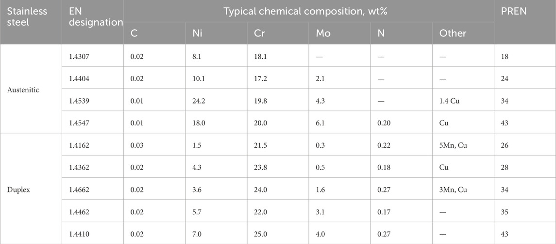
Table 1. Typical chemical compositions of the stainless steels investigated (wt%). The alloys are given in order of increasing PREN (%Cr+3.3x%Mo+16x%N) within each group.

2.2 Electrochemical pitting corrosion testing

The results from five electrochemical methods were investigated to develop a robust method for constructing pitting engineering diagrams:

Method 1: Potentiodynamic polarization technique (Pitting potential measurements, E_pit) at a constant temperature.

Method 2: Potentiostatic critical pitting temperature (CPT).

Method 3: Potentiostatic measurement at a constant temperature for 2 h.

Method 4: Sweep potential (from E_OCP to E_app) followed by potentiostatic polarization at constant temperature for 2 h.

Method 5: Sweep potential (from E_OCP to E_app) followed by potentiostatic polarization at constant temperature for 30 days.

In method 5, two selected potentials (E_app) were set for defining the pitting no pitting boundaries in this study: 1) 150 mV vs. SCE for simulating sterile tap water and 2) 400 mV vs. SCE for simulating slightly chlorinated water or water with some bacterial activity (Mameng et al., 2017; Outokumpu, 2023). Measurements 2–4 were performed at 400 mV vs. SCE.

2.2.1 Test parameters

The electrochemical measurements were performed in sodium chloride solutions (NaCl) with chloride ion concentrations between 10 and 100,000 ppm (mg/L) at different temperatures ranging from 10°C ± 1°C to 80°C ± 1°C. Methods 1–4 were performed in the Avesta cell (ASTM G61-86, 2018; ASTM G150-18, 2018) when the chloride content was 1,000 ppm or higher, as shown in Figure 1A. For the tests performed in chloride concentrations below 1,000 ppm, a hydrophobic washer (silicone-based dental putty; Provo Novil Putty-Soft fast set, Heraeus†) with Teflon spray (Cargo-Oil) was used to cover the crevice area of the specimen. The Avesta cell has been designed to avoid the formation of microcrevices and to eliminate their consequences. This is achieved by letting distilled water replace the chloride solution in the microcrevice between the specimen and the specimen holder (Ovarfort, 1988). Method 5’s long-term measurement was performed in an electrochemical cell, which was set up from glass cylindrical reaction vessels with an O-ring flange and glass lid with five necks, as shown in Figure 1B. An external heating unit was used to perform the measurements at the desired temperature.

Figure 1

Figure 1. The experimental setup, (A) Avesta Cell and (B) Cylindrical reaction vessel.

Before exposure to the test solution, the specimens’ exposed surfaces and edges were wet ground using SiC paper to 320 and 500 grit, respectively. After the grinding, the specimens were left in the air to passivate for at least 18 h before testing. For Method 5, the specimens were soldered with an electric cable using a rivet, which was then covered with MS Polymer™† “modified silicone” (i.e., the entire sample was not covered) and left in air for at least 24 h before testing. Immediately before the experiment, the specimens were cleaned with ethanol. The working electrode’s potential versus a SCE reference electrode was measured. The auxiliary electrode was a platinum (Pt) mesh. Dissolved oxygen was kept low by bubbling nitrogen through the sodium chloride solution during the experiment, except in Method 5. The test parameters used for the five different test methods are summarized in Table 2.

Table 2

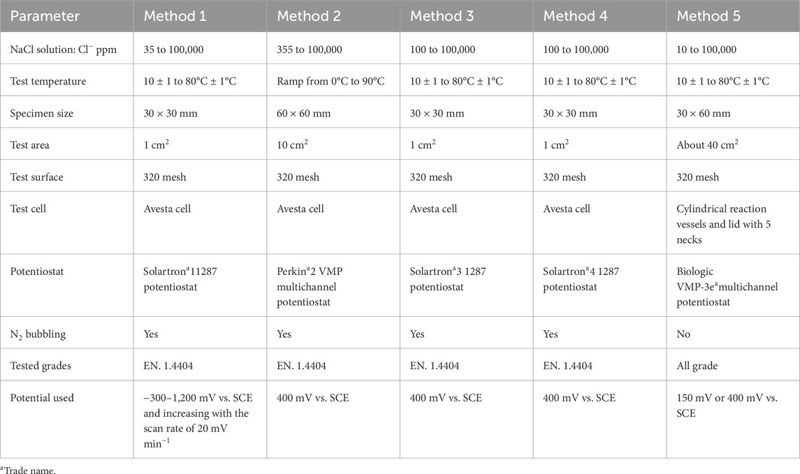
Table 2. The test parameter and tested grade.

2.2.2 Method 1: potentiodynamic polarization (pitting potential measurements, E_pit)

Before each polarization measurement, the open circuit potential (E_OCP) was measured for 10 min in the test solution. The polarization started at −300 mV vs. SCE, and the potential was thereafter increased at a scan rate of 20 mV·min⁻¹. E_pit was defined as the potential where the current exceeds 100 μA·cm⁻² and remains above this level for at least 1 min (Fielder and Johns, 1989; Mameng et al., 2014; Mameng et al., 2017), as shown in Figure 2A. In case no breakdown potential was observed, the polarization was ended at 1,200 mV vs. SCE. Triplicate samples were tested in most cases, with a maximum difference of <100 mV in the obtained E_pit. If more significant differences were observed, additional measurements were made.

Figure 2

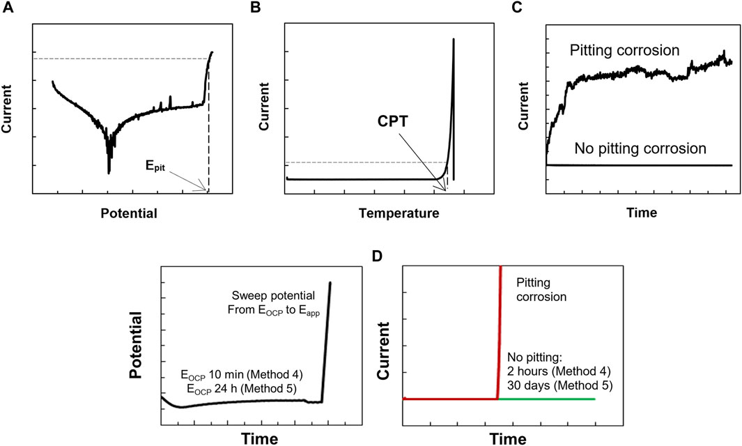
Figure 2. Schematic curves obtained from 5 different methods. (A) method 1, (B) method 2, (C) method 3, (D) methods 4 and 5.

2.2.3 Method 2: potentiostatic critical pitting potential (CPT)

The E_OCP was measured at 0°C for 10 min before each measurement. From the initial temperature of 0°C, the temperature of the test solution was heated at a rate of 1°C·min⁻¹ while the potential was held constant (at 400 mV vs. SCE). The current was monitored during the whole test, see Figure 2B. Triplicate specimens were used to determine the CPT.

2.2.4 Method 3: potentiostatic measurement at a constant temperature

The E_OCP was measured at the desired temperature for 10 min before each measurement. Then, a constant potential (400 mV vs. SCE) was applied. The current was monitored for a test period of 2 h. Triplicate specimens were tested to confirm the absence of pitting corrosion whereas only one test was sufficient to confirm the pitting corrosion (see Figure 2C).

2.2.5 Method 4: sweeping the potential (from E_OCP to E_app) followed by potentiostatic polarization at a constant temperature for 2 h

The electrochemical procedure for Method 4 was set up in three different steps. The first step was the E_OCP measurement for 10 min at the desired temperature. The second step was to sweep the potential (scan rate 20 mV·min⁻¹), starting from the E_OCP to the set potential (400 mV vs. SCE). The third step was to keep the constant potential (400 mV vs. SCE) and monitor the current during the 2-h test period, as shown in Figure 2D. Triplicate specimens were tested to confirm the absence of pitting corrosion whereas only one test was sufficient to confirm the pitting corrosion.

2.2.6 Method 5: sweeping the potential (from E_OCP to E_app) followed potentiostatic polarization at a constant temperature for 30 days

The electrochemical procedure for Method 5 was also set up in three different steps. The first step was the E_OCP measurement for 24 h. The second step was to sweep the potential (scan rate 20 mV·min⁻¹), starting from the E_OCP to the set potential (either 150 or 400 mV vs. SCE). The third step was to keep the potential constant at either 150 or 400 mV vs. SCE. The current was monitored during the 30-day test period, as shown in Figure 2D. Only one specimen was sufficient to determine whether pitting corrosion was present or not.

Pitting on the surface and the absence of crevice corrosion were confirmed after the tests (Methods 1–5) using a microscope at ×20 magnification. In the case of the observation of crevice corrosion (methods 1–4) or edge corrosion (method 5), the corresponding tests were discarded. The criterion for pit initiation in all 5 methods used here is the current exceeding 100 μA cm⁻².

3 Results

3.1 Pitting diagrams based on pitting potential (E_pit) data–method 1

Potentiodynamic anodic polarization curves were used to determine the E_pit for EN 1.4404 at different chloride concentrations and temperatures. The typical curve for the evaluation of E_pit is illustrated in Figure 2A. E_pit was defined at the point where the current exceeds 100 μA·cm². The reason for using this current density and not 10 μA·cm⁻² is that the so-called metastable pits could also result in current peaks above 10 μA·cm⁻². Hence, clear identification of stable pitting required a higher threshold (Mameng et al., 2017). Figure 3 shows the effect of chloride concentration and temperature on E_pit and illustrates that the E_pit decreases when the chloride concentration and/or temperature increase. The breakdown potential plot vs. a wide range of temperatures is typically observed as a reversed S-shaped curve (Meguid et al., 1998; Mameng et al., 2017). As can be seen from this figure, at the lowest chloride level investigated the breakdown potential is high (above 1,200 mV vs. SCE). The electrochemical reaction taking place here is transpassive corrosion and not pitting corrosion. At higher chloride concentrations and temperatures, the breakthrough potential is the result of pitting corrosion.

Figure 3

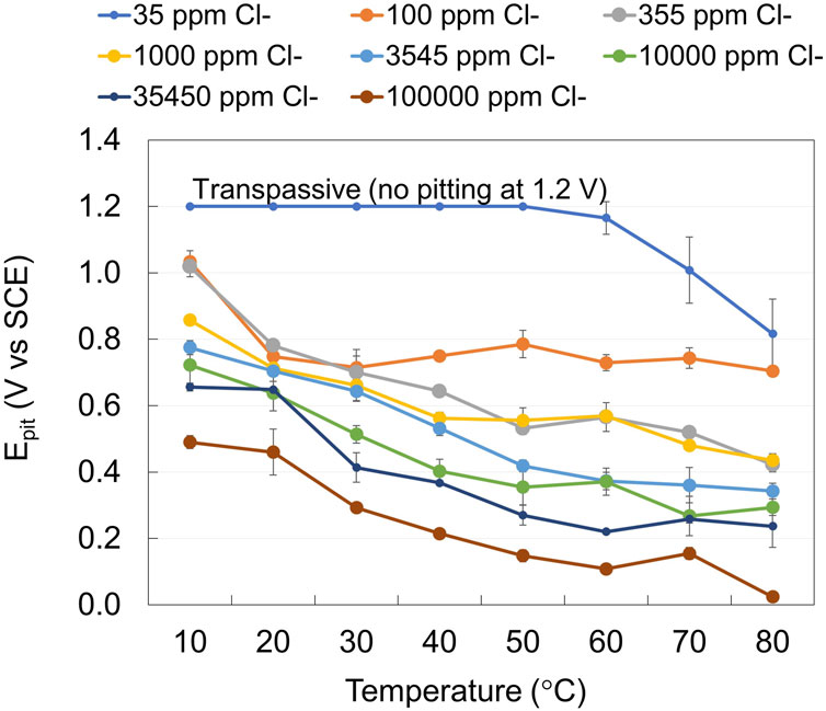
Figure 3. Effect of chloride concentration and temperature on E_pit for EN 1.4404.

The E_pit results obtained from the potentiodynamic polarization curves were used to define the limits in terms of chloride concentration and temperature where the risk for pitting corrosion exists. The idea of pitting engineering diagrams based on E_pit measurements has been presented earlier (Fielder and Johns, 1989; Lu et al., 1993; Laycock and Newman, 1998). In the present study, the diagrams were obtained by mapping the regions where pitting occurs at selected potentials, as shown in Figure 4. The solid points indicate that E_pit is equal to or lower than 400 mV vs. SCE, whereas open points indicate E_pit at higher potentials. The results in Figure 4 show that E_pit data gives sufficiently small standard deviations for evaluating a broad range of chloride concentrations and temperatures. The pitting diagram obtained from Method 1 could potentially be useful for material selection in slightly chlorinated water or the presence of biofilm in the water system. It can also serve as a basis for assessing corrosion risks in service, particularly if the effect of additional environmental components can be considered.

Figure 4

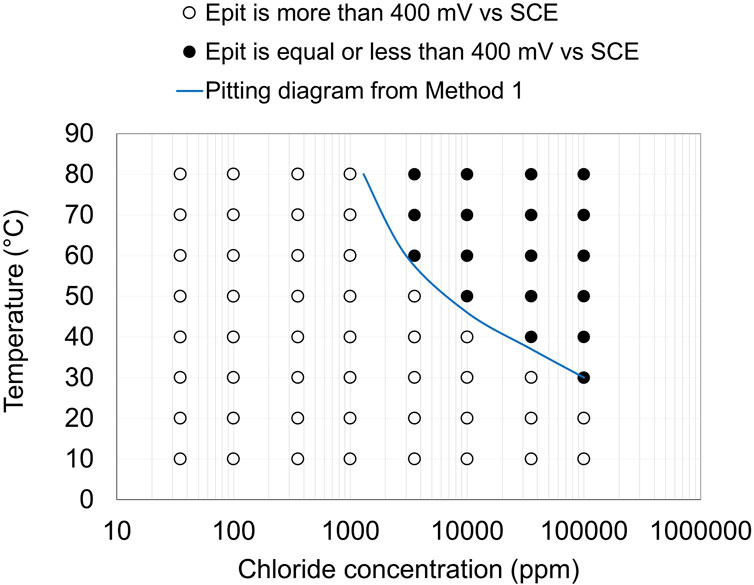
Figure 4. Pitting engineering diagram based on E_pit data (Method 1) for EN 1.4404.

3.2 Pitting diagram based on critical pitting temperature (CPT)–method 2

Raising the temperature at a constant potential to determine the critical pitting temperature (CPT) is well established and included in the standard test method ASTM G150 (ASTM G150-18, 2018). The pitting engineering diagram for EN 1.4404 was constructed using the CPT results. Method 2 follows the ASTM G150 standard except that the measurements were performed at 400 mV rather than 700 mV vs. SCE level described in the standard. Moreover, NaCl concentrations other than 1 M were used to construct the pitting diagram based on method 2. The current density vs. temperature curve and the corresponding pitting engineering diagram constructed based on the CPT data at the applied potential of 400 mV vs. SCE for EN 1.4404 are illustrated in Figure 5. The results show that CPT data give sufficiently small standard deviations for tests performed at 1,000 ppm or higher chloride concentrations. Method 2 has experimental challenges at low chloride concentrations (<1,000 ppm Cl⁻), as unwanted crevice corrosion is easily initiated, especially for the low alloyed stainless steel tested grade.

Figure 5

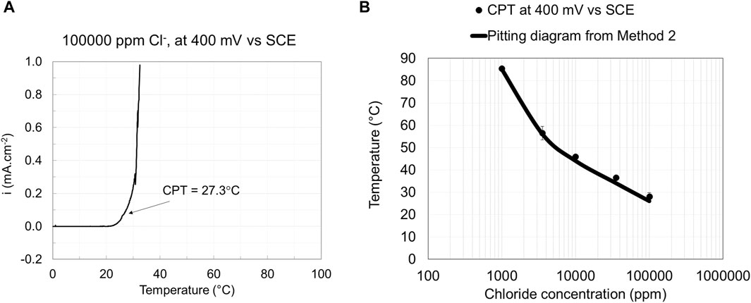
Figure 5. Current vs. temperature curve (A) and pitting engineering diagrams (B) based on data obtained from Method 2.

3.3 Pitting diagram based on potentiostatic polarizations at constant temperature for 2 h–method 3

In method 3 a constant potential (400 mV vs. SCE) was applied to the specimen, and the solution was kept at a constant desired temperature. The current density was monitored as a function of time during the whole experiment. The test was repeated for solutions with different chloride ion concentrations, temperatures, and steel grades, as seen in Figure 6A and the corresponding pitting engineering diagram was obtained (Figure 6B). The advantage of this method compared to method 2 is that it can also be used at low chloride levels (<1,000 ppm Cl⁻).

Figure 6

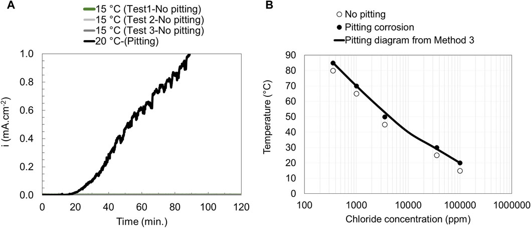
Figure 6. Current vs. time curves (A) and pitting engineering diagrams (B) based on data obtained from method 3 for EN 1.4404.

3.4 Pitting diagram based on potential sweep (from E_OCP to E_app) followed by potentiostatic polarization at constant temperature for 2 h–method 4

Method 4 is the modified version of Method 3 in which the potential is swept slowly from the E_OCP to 400 mV vs. SCE after which the potential is kept unchanged for 2 h. The current density is monitored as a function of time during the whole experiment. The potentiostatic polarization curves obtained from Method 4 and the corresponding pitting engineering diagrams are shown in Figure 7.

Figure 7

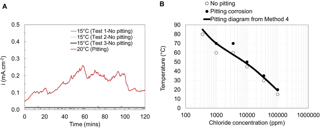
Figure 7. Current vs. time curves (A) and pitting engineering diagrams (B) based on data obtained from method 4 for EN 1.4404.

3.5 Pitting diagram based on potential sweep (from E_OCP to E_app) followed by potentiostatic polarization at constant temperature for 30 days–method 5

The test procedure of Method 5 is similar to Method 4, but there is a difference in the testing duration during which the potential is kept constant at either 150 mV or 400 mV vs. SCE for 30 days. Figures 8A–C show the current vs. time curves obtained from Method 5 tested in 100 ppm Cl⁻ at different temperatures for EN 1.4404. The occurrence of pitting corrosion is seen as an increase in the current density, as illustrated in Figures 8B, C. The tests showed an increase in current density after about 230 and 65 h, respectively. In contrast to the tests at higher temperatures, no corrosion was seen at 60°C, maintaining a low current density throughout the test. The pitting engineering diagrams based on Method 5 is shown in Figure 8D. After testing, the visual and microscopy examination indeed confirmed that pitting had occurred at 70°C and 80°C (Figures 9B, C), whereas the sample tested at 60°C (Figure 9A) shows no pitting corrosion attack. Figure 9C indicates some pitting close to the edge. Nevertheless, examination of the pit initiation region (using a needle) indicated that the pit indeed was initiated from the surface.

Figure 8

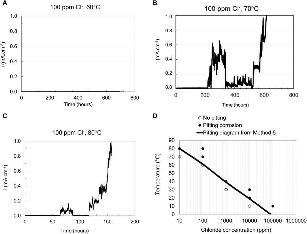
Figure 8. Obtained current vs. time curves from Method 5 (A–C) tested in 100 ppm chloride ion concentration at different temperatures and Pitting engineering diagrams based on data from Method 5 (D).

Figure 9

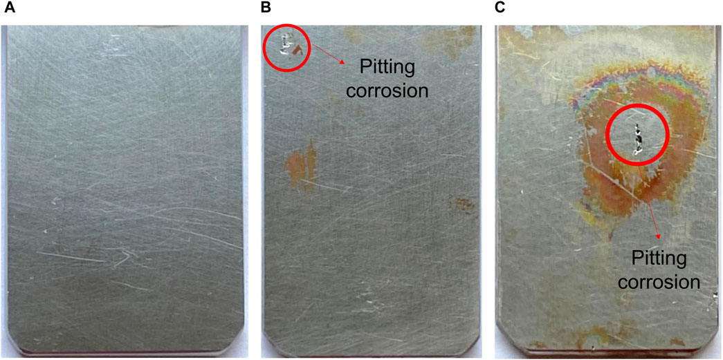
Figure 9. The appearance of EN 1.4404 and micro photo of corrosion attacked on EN 1.4404 after testing under Method 5. The sample dimensions are 60 × 30 × 3 mm. (A) tested at 60°C, (B) tested at 70°C, and (C) tested at 80°C.

A summary of the results for EN 1.4404 stainless steel based on Methods 1–5 at different chloride concentrations is shown in Table 3.

Table 3

Table 3. Results based on Methods 1–5 for EN 1.4404.

3.6 Pitting diagrams at two oxidation potentials of the water system

To assess the relevance of the pitting engineering diagrams to long-term service performance, long-term laboratory testing (Method 5) was performed on a wide range of stainless steel grades to simulate the corrosive environments. In these tests, two oxidation potentials of the water system were selected based on those presented earlier (Fielder and Johns, 1989; Mameng et al., 2014; Mameng et al., 2017). In the current work, a primary consideration was that 150 mV vs. SCE corresponds to simulating sterile tap water. In comparison, 400 mV vs. SCE corresponds to slightly chlorinated water or water with some biological activity. Nine different stainless steel grades were tested in different chloride ion concentrations and temperatures at two oxidation potentials of the water system.

The long-term test results on austenitic and duplex grade stainless steels are summarized in Tables 4, 5, respectively. Samples were examined after exposure to the chloride solutions with different temperatures for 30 days. For each test condition and material, it is investigated whether the material suffered pitting corrosion on the tested surface. The pitting corrosion on the edges of the tested specimens was disregarded. Where corrosion occurs, the cells are filled red (X); whereas no corrosion is indicated as green cells (O).

Table 4

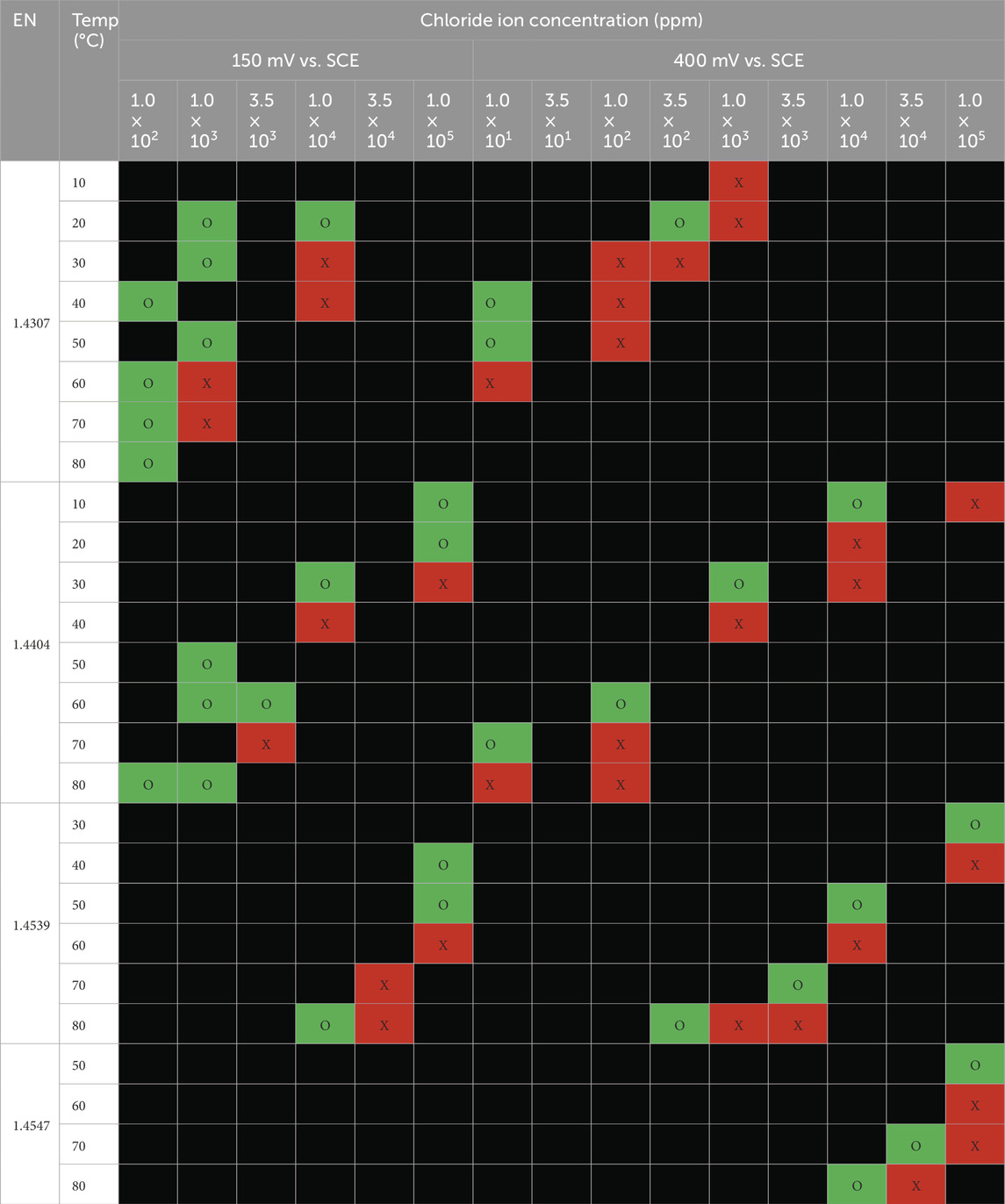
Table 4. Summary of visible pitting corrosion for austenitic stainless steel grades (X-Red cells = pitting corrosion and the pit depth ≥25 microns, O-Green cell = no corrosion and Black cell = not tested).

Table 5

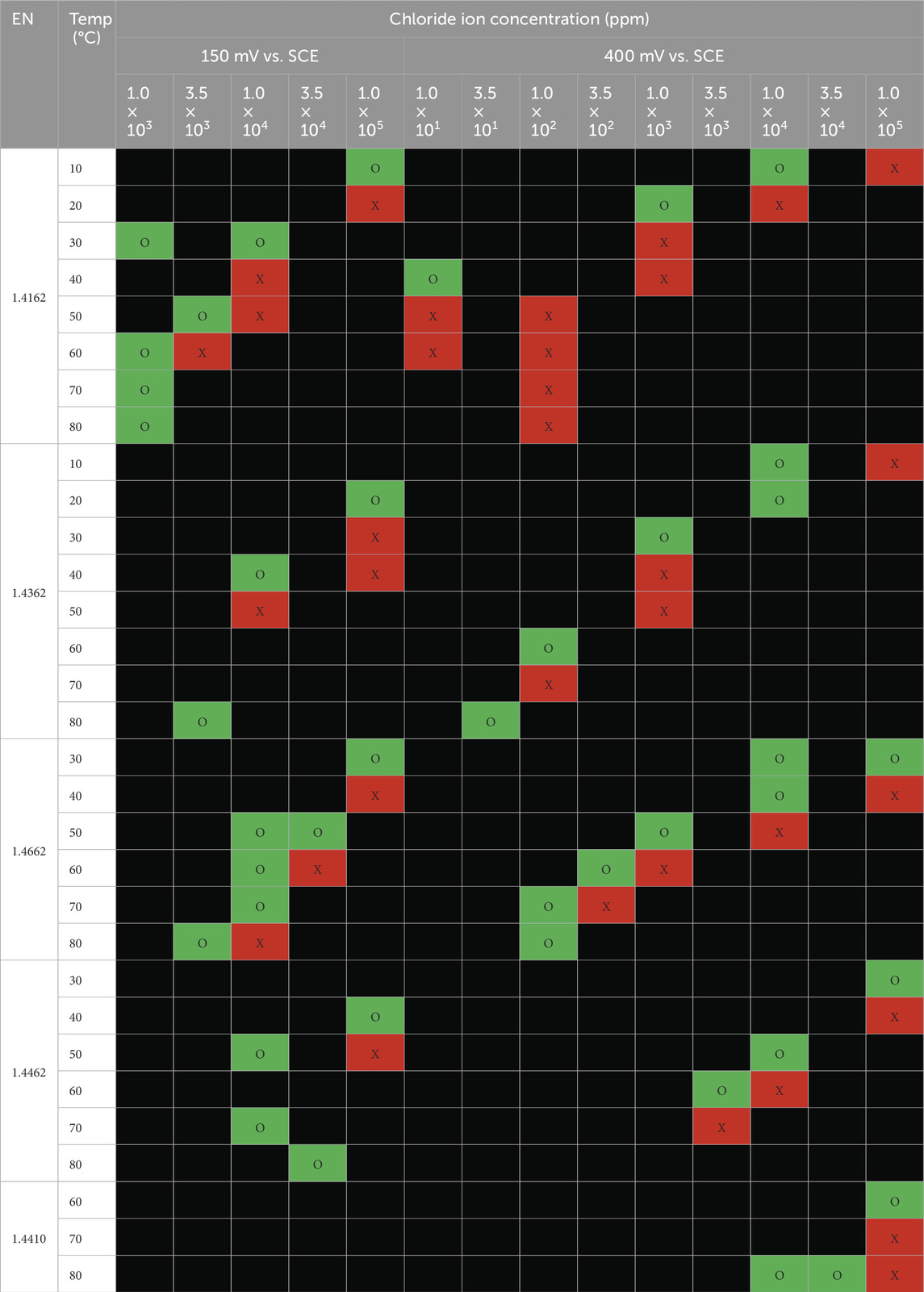
Table 5. Summary of visible pitting corrosion for duplex stainless steel grades (X-red cells = pitting corrosion and the pit depth ≥25 microns, O-green cell = no corrosion and Black cell = not tested).

4 Discussion

4.1 Comparison to electrochemical measurements

Based on the result, the obtained pitting engineering diagrams from different test methods show similarities and differences regarding the limiting condition for pitting corrosion (i.e., the border for pitting and no pitting) of stainless steel. Five electrochemical methods were performed on samples of the same materials in identical test solutions to construct and assess the diagrams’ accuracy. The most notable feature from the diagrams obtained from the five methods is the curve-shaped form (see Figure 10) compared with the straight lines or S-shape curves usually seen in other studies (Mameng et al., 2017; Mameng and Pettersson, 2014). The fundamental trends are very similar for the five methods. An explanation for the curved shape boundary between pitting and no pitting regions in the engineering diagrams, shown in Figures 10–12, is that the pitting initiation process is impeded by the lower availability of chloride ions at sufficiently low chloride contents. An increase in temperature is to be expected to have several impacts on pitting initiation and growth. Firstly, the rate of chemical reactions, including metal dissolution increases with temperature, as does the pit growth rate (Sedriks, 1986). Additional effects of temperature include faster diffusion of various species through the oxide film as well as into and out of the pit (Leckie and Uhlig, 1966; Sedriks, 1986; Moayed et al., 2003). Once the critical level of chloride ion and temperature is exceeded, the fast dissolution rate will occur, leading to pitting initiation and propagation (ASTM G61-86, 2018; ASTM G150-18, 2018).

Figure 10

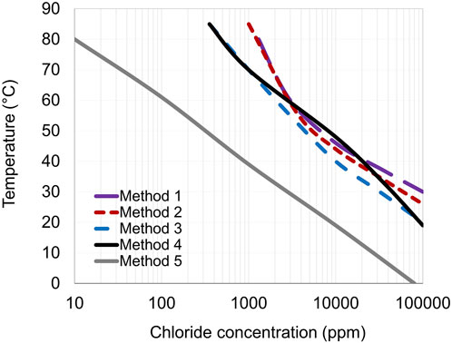
Figure 10. Pitting engineering diagrams from five different methods for EN 1.4404.

Figure 11

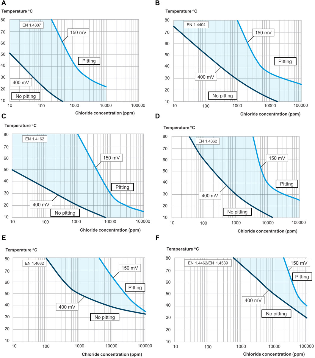
Figure 11. Pitting engineering diagrams for different grades of stainless steel (A–F) indicating the maximum temperatures and chloride concentrations allowed for two different kinds of water system. 150 mV vs. SCE simulates sterile tap water, and 400 mV vs. SCE simulates slightly chlorinated water or water with some biological activity. The light blue area between the lines indicates the uncertainty of the borders between pitting and no pitting.

Figure 12

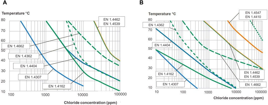
Figure 12. Pitting engineering diagrams indicating the maximum temperatures and chloride concentrations allowed for two different water systems. (A) 150 mV vs. SCE simulates sterile tap water and (B) 400 mV vs. SCE simulating slightly chlorinated water or water with some biological activity.

Even though the different methods result in a similar shape of the borderlines between pitting and no pitting regions, it is evident that they provide quite different results (see Figure 10). The borderlines (pitting limit) obtained from methods 1–5 differ due to the protocols of the electrochemical method used; i.e., the procedure used for applied potential and incubation time (testing duration). These parameters may affect the passive film’s stability and performance (Olsson and Landolt, 2003; Wegrelius and Olefjord, 1993). It is well known that the passive film breakdown depends on the induction time for pit initiation. It appears that the existence of an incubation time means that the relatively high rate of potential change (dE/dt) for the potentiodynamic technique at constant temperature (Method 1) shifts the E_pit to higher values compared to an applied constant potential at a given temperature (Methods 3, 4, and 5). Accordingly, Method 1 seems to give too optimistic data due to the high sweep rate (20 mV/min) of the potential (almost no induction time), and it is very time-consuming as it requires many tests and specimens.

In the case of CPT measurements (Method 2), the time for the temperature to reach CPT gives the passive film a chance to adjust its properties. The passive film is modified during the time spent at temperatures below the CPT. Hence, the trend is a more stable passive layer that breaks down at higher temperatures than those obtained in Methods 3 and 4. Nevertheless, the relatively fast rate of the temperature change most probably increases the CPT to slightly higher values. The diagram obtained from Method 2 seems to give data that is too optimistic due to the high-temperature ramp rate (almost no induction time). Comparing the border lines between Method 1 and Method 2 (Figure 10) shows a general agreement between the results of the two tests for grade EN 1.4404. Nevertheless, there is less than a 5°C difference between Method 1 and Method 2 (see Table 3). As described earlier, the advantage of the potentiostatic CPT (Method 2) is that it gives results in a short period and with a limited number of tests.

The results obtained from Methods 3 and 4 give more conservative data than Methods 1 and 2 and can be utilized even at low chloride concentrations (<1,000 ppm Cl⁻). There is a relatively good agreement between the boundary lines developed from Methods 3 and 4. The diagrams from Method 3 are slightly more conservative than Method 4, as the specimens from Method 4 are subject to a gradual potential increase from the E_OCP to E_app (with a scan rate of 20 mV·min⁻¹). This sweep potential procedure strengthens the passive film compared to Method 3. Hence, the breakdown of a more stable passive layer (formed in Method 4) occurs at higher temperatures than that in Method 3. However, for EN 1.4404, the borderline from Method 3 was quite similar to Method 4 at tested low and high chloride levels. At the intermediate chloride levels, the borderline was similar to Methods 1 or 2. Comparing the borderline between Method 5 and other Methods confirms the general agreement between these methods, but as seen in Figure 10, the most conservative borderline is obtained from Method 5. Method 5 clearly shows the importance of an induction time for pit initiation (more than 2 h), giving the most conservative yet most realistic data. Even though Method 5 is time-consuming, it provides more confidence when predicting in-service corrosion performance.

4.2 Pitting engineering diagrams for two different water systems

A long-term electrochemical method was used to determine the pitting corrosion resistance of a range of stainless steels in aqueous solutions. It represents a matrix of the critical environmental parameters that strongly influence pitting corrosion performance, i.e., the system’s chloride ion concentration, temperature, and oxidizing power of the medium. The data generated by this method have been used to construct pitting engineering diagrams (see Figures 11, 12). The idea of engineering diagrams based on long-term laboratory testing has been presented earlier (Fielder and Johns, 1989; Mameng et al., 2014; Mameng et al., 2017). The result from the two potentials is included in the same diagram, one for each stainless steel grade, as shown in Figure 11. The diagrams show a significant relationship between pitting corrosion behavior, environmental conditions, and material parameters. The dashed area between the lines indicates the uncertainty of the borders between pitting and no pitting. The differences in the borderline of the different oxidizing potentials of the water system are noticeable (Figure 11). The lines in the diagrams for 400 mV vs. SCE have a similar trend to 150 mV_SCE but are more conservative. The borderline (pitting limit) differs due to the oxidizing effect in these parameters, which may affect the passive film’s stability and performance (Bardwell et al., 1992; Wegrelius and Olefjord, 1993; Olsson and Landolt, 2003; Fredriksson et al., 2010). In Figure 12, the results obtained on all investigated stainless steel grades are shown in the same diagram, but only one potential per diagram. Stainless steel grades EN 1.4547 and EN 1.4410 are only represented in Figure 12B, as they are too corrosion-resistant at a lower potential of 150 mV vs. SCE (i.e., Figure 12A). It is seen that the alloying composition of the different stainless steels affects the limits for the pitting corrosion resistance. Two types of pitting engineering diagrams have been constructed based on the water system’s oxidation potential (E_OCP). As was mentioned earlier, 150 mV vs. SCE corresponds to the upper limit of the potential exerted on stainless steel when exposed to sterile tap water. In comparison, whereas 400 mV vs. SCE represents slightly chlorinated water or water with some biological activity. In practice, The maximum potential is typically in the range 200–250 mV vs. SCE for a drinking water system (Mameng and Pettersson, 2014; Mameng and Pettersson, 2011) and about 300 mV vs. SCE for a water heater system (Johansson and Mameng, 2014). For chlorinated water, the potential of the system depends on the chlorine level: it has been reported that the maximum potential is about 400 mV vs. SCE for 0.2 ppm chlorine and about 500 mV vs. SCE for 0.5 ppm chlorine (Larché et al., 2013; Mameng and Alfonsson, 2012). However, the main point to consider when using the diagrams is that the oxidation potential of the water system may not always be known. It should be noted that these diagrams only give approximate guidance as to the suitability of stainless steel. The final choice of stainless steel, however, will depend on several other factors, such as different surface conditions and the presence of other environmental species or crevice design or weld. It is important to remember that the actual service conditions may differ considerably from those used to design the diagram. One example is if crevices or weld oxides are present in the construction. Crevice corrosion typically initiates more easily than pitting corrosion, so the lines in the diagram are shifted towards more conservative values. Another example is if some contaminants are present in the water, as certain substances could activate, and others could inhibit the corrosion process. The extension of engineering diagrams in which these factors are considered is out of the scope of this work but is ongoing in our laboratory.

5 Conclusion

The aim of this work was to develop a practical tool which can be used for the selection of stainless steel at a wide range of temperature and chloride ion concentrations. The alloying composition of stainless steel, chloride ion, temperature, and the water system’s oxidation potential are important parameters affecting the stainless steel pitting resistance. Two sets of potentials, 150 mV and 400 mV vs. SCE were selected to represent the common scenarios in sterile tap water and slightly chlorinated water or water with some biological activity, respectively. The pitting engineering diagram was constructed based on an extensive electrochemical laboratory testing matrix. All the electrochemical methods used in this study adequately construct pitting engineering diagrams showing the boundaries between pitting and no pitting in terms of chloride concentration, temperature, and the water system’s oxidation potential. All test methods could potentially be used for ranking purposes. Nevertheless, identifying the most appropriate testing method, which closely corresponds to real application, was put in the focus. The comparison between the results obtained from different methods indicated that long-term electrochemical method (identified as method 5, which allows a longer incubation period) was most successful in constructing pitting diagrams showing the boundaries between pitting and no pitting in terms of chloride concentration, temperature, and the water system’s oxidation potential. These results will enable reliable material selection for different applications of stainless steel where it is exposed to chloride-containing media at different temperatures and concentrations. Although the pitting engineering diagrams are a very useful tool to aid material selection, it is important to realize that additional factors, such as different surface conditions and the presence of other environmental species or crevice design or weld, will affect the exact position of the boundaries.

Data availability statement

The raw data supporting the conclusion of this article will be made available by the authors, without undue reservation.

Author contributions

SuH: Conceptualization, Data curation, Formal Analysis, Methodology, Visualization, Writing–original draft, Writing–review and editing. LW: Resources, Supervision, Writing–review and editing. SaH: Investigation, Supervision, Validation, Visualization, Writing–review and editing.

Funding

The author(s) declare that no financial support was received for the research, authorship, and/or publication of this article.

Acknowledgments

The authors wish to thank Outokumpu Stainless Steel AB. Björn Helmersson and Elisabeth Johansson are acknowledged for valuable discussions. Jochen Muller, Christian Stankewitz, Annika Almén, and Maria Almén are thanked for performing the electrochemical test and sample preparation.

Conflict of interest

Authors SuH and LW were employed by Outokumpu Stainless Steel AB. Author SaH was employed by Outokumpu Nirosta GmbH.

The handling editor TK declared past co-authorship with the authors SuH and LW.

Publisher’s note

All claims expressed in this article are solely those of the authors and do not necessarily represent those of their affiliated organizations, or those of the publisher, the editors and the reviewers. Any product that may be evaluated in this article, or claim that may be made by its manufacturer, is not guaranteed or endorsed by the publisher.

References

ASTM G150-18 (2018). Standard test method for electrochemical critical pitting temperature testing of stainless steels and related alloys. West Conshohocken: ASTM.

Google Scholar

ASTM G61-86 (2018). Standard test method for conducting cyclic potentiodynamic polarization measurements for localized corrosion susceptibility of iron-, nickel-, or cobalt-based alloys. West Conshohocken: ASTM.

Google Scholar

Bardwell, J. A., Sproule, G. I., MacDougall, B., Graham, M. J., Davenport, A. J., and Isaacs, H. S. (1992). In situ XANES detection of Cr(VI) in the passive film on Fe-26Cr. J. Electrochem Soc. 139 (2), 371–373. doi:10.1149/1.2069224

CrossRef Full Text | Google Scholar

Fernández-Domene, R. M., Blasco-Tamarit, E., García-García, D. M., and García-Antón, J. (2014). Effect of alloying elements on the electronic properties of thin passive films formed on carbon steel, ferritic and austenitic stainless steels in a highly concentrated LiBr solution. Thin Solid Films 558, 252–258. doi:10.1016/j.tsf.2014.03.042

CrossRef Full Text | Google Scholar

Fielder, J. W., and Johns, D. R. (1989). Pitting corrosion engineering diagrams for stainless steels. Br. Steel Tech., 9–14.

Google Scholar

Fredriksson, W., Edström, K., and Olsson, C.-O. A. (2010). XPS analysis of manganese in stainless steel passive films on 1.4432 and the lean duplex 1.4162. Corros. Sci. 52 (7), 2505–2510. doi:10.1016/j.corsci.2010.03.014

CrossRef Full Text | Google Scholar

Johansson, E., and Mameng, S. H. (2014). Long-term corrosion test of stainless steel for water heater applications.

Google Scholar

Larché, N., Thierry, D., Labelleur, C., Wijesingue, S. L., and Zixi, T. (2013). Evaluation of corrosion risks with the use of high alloy stainless steels in seawater applications–effect of service conditions on corrosion potential and cathodic efficiency. Maastricht: Stainless Steel World.

Google Scholar

Laycock, N. J., and Newman, R. C. (1998). Temperature dependence of pitting potentials for austenitic stainless steels above their critical pitting temperature. Corros. Sci. 40 (6), 887–902. doi:10.1016/s0010-938x(98)00020-1

CrossRef Full Text | Google Scholar

Leckie, H. P., and Uhlig, H. H. (1966). Environmental factors affecting the critical potential for pitting in 18–8 stainless steel. J. Electrochem Soc. 113 (12), 1262. doi:10.1149/1.2423801

CrossRef Full Text | Google Scholar

Lu, Y. C., Ives, M. B., and Clayton, C. R. (1993). Synergism of alloying elements and pitting corrosion resistance of stainless steels. Corros. Sci. 35 (1), 89–96. doi:10.1016/0010-938x(93)90137-6

CrossRef Full Text | Google Scholar

Mameng, S., and Pettersson, R. (2011). “Localized corrosion of stainless steel depending on chlorine dosage in chlorinated water,” in Proceedings Eurocorr 2011, Stockholm, Sweden, 4-8 September 2011 (Maastricht: Eurocorr).

Google Scholar

Mameng, S. H., and Alfonsson, E. (2012). Possibilities and limitations of austenitic and duplex stainless steels in chlorinated water systems. Nucl. Exch. Mag.

Google Scholar

Mameng, S. H., Bergquist, A., and Johansson, E. (2014). Corrosion of stainless steel in sodium chloride brine solutions. Corrosion.

Google Scholar

Mameng, S. H., and Pettersson, R. (2014). “Limiting conditions of pitting corrosion for lean duplex stainless steel as a substitute for standard austenitic grades,” in Proceedings EUROCORR Conference, Pisa, Italy, 8-12 September 2014 (Pisa: EUROCORR).

Google Scholar

Mameng, S. H., Pettersson, R., and Jonson, J. Y. (2017). Limiting conditions for pitting corrosion of stainless steel EN 1.4404 (316L) in terms of temperature, potential and chloride concentration. Mater. Corros. 68 (3), 272–283. doi:10.1002/maco.201609061

CrossRef Full Text | Google Scholar

Meguid, E., Mahmoud, N. A., and Gouda, V. K. (1998). Pitting corrosion behaviour of AISI 316L steel in chloride containing solutions. Br. Corros. J. 33 (1), 42–48. doi:10.1179/bcj.1998.33.1.42

CrossRef Full Text | Google Scholar

Moayed, M. H., Laycock, N. J., and Newman, R. C. (2003). Dependence of the critical pitting temperature on surface roughness. Corros. Sci. 45 (6), 1203–1216. doi:10.1016/s0010-938x(02)00215-9

CrossRef Full Text | Google Scholar

Olsson, C.-O. A. (1995). The influence of nitrogen and molybdenum on passive films formed on the austenoferritic stainless steel 2205 studied by AES and XPS. Corros. Sci. 37 (3), 467–479. doi:10.1016/0010-938x(94)00148-y

CrossRef Full Text | Google Scholar

Olsson, C.-O. A., and Landolt, D. (2003). Passive films on stainless steels—chemistry, structure and growth. Electrochim Acta 48 (9), 1093–1104. doi:10.1016/s0013-4686(02)00841-1

CrossRef Full Text | Google Scholar

Outokumpu (2023). Outokumpu corrosion handbook. 12th ed. Helsinki: Outokumpu.

Google Scholar

Ovarfort, R. (1988). New electrochemical cell for pitting corrosion testing. Corros. Sci. 28 (2), 135–140. doi:10.1016/0010-938X(88)90090-X

CrossRef Full Text | Google Scholar

Sedriks, A. J. (1986). <i>Plenary lecture—1986:</i>Effects of alloy composition and microstructure on the passivity of stainless steels. Corrosion 42, 376–389. doi:10.5006/1.3584918

CrossRef Full Text | Google Scholar

Wegrelius, L., and Olefjord, I. (1993). Passivation of High Alloyed Stainless Steel in HCl at 22°C and 65°C. 12th Int. Corrosion 1993, paper no. 3887 (Houston, TX: NACE).

Google Scholar