A framework for computer-aided high performance titanium alloy design based on machine learning

1 Introduction

The application of titanium-containing alloys, such as titanium alloy, titanium-niobium alloy, and high entropy alloy, has been extensively observed in the fields of aerospace, navigation, and medicine (Cheng et al., 2021; Cheng et al., 2022; Guo et al., 2023; Liu et al., 2023; Kang et al., 2024; Shen et al., 2024). Among these alloys, titanium alloy stands out due to its exceptional specific strength, corrosion resistance, low-temperature tolerance, high-temperature endurance, and remarkable biocompatibility. In the aerospace field, titanium alloy has been mainly used in aircraft structural components, lips, tubes, fasteners, satellite shells, rocket tubes, and rocket engine shells, etc., especially, the proportion of titanium alloy in the structure of the fifth-generation advanced fighter F-22 in the United States has reached 41% (Boyer, 1995; Liu et al., 2015; Liu et al., 2020). In the field of navigation, titanium alloy has been used in ship structural parts, submarine shells, marine water pipelines, etc. (Chen et al., 2005; Song et al., 2020). Moreover, in the medical field, titanium alloy serves as a crucial material for artificial substitutes or implants including joints, craniofacial structures, and dental implants (Hanawa, 2019; Lourenço et al., 2020; Sarraf et al., 2022). The demand for new high-performance titanium alloys is increasing due to wide-ranging applications, particularly in the aerospace field where high strength and toughness are emphasized, the marine field where corrosion resistance is prioritized, and the biomedical field where a high elastic modulus is sought after.

There are two approaches in traditional material design, namely, manual design and structural search. Manual design involves the intuitive creation of new materials based on expert knowledge and experience, while structural search entails designing novel materials through structure and calculation methods such as combination experiments, phase diagram calculations (CALPHAD), and density functional theory (DFT) (Ji et al., 2014; Mao et al., 2017; Rao et al., 2022a; Tian et al., 2022; Song et al., 2023). However, these traditional methods require extensive calculations and experimental trial-and-error processes with high demands for expertise from material designers, resulting in elevated development costs and low efficiency.

In the era of rapid advances in data-driven and artificial intelligence technologies, computer-aided design (CAD) of novel materials has become feasible (Ren et al., 2018; Yu et al., 2019; Deng et al., 2020; Wahl et al., 2021; Rao et al., 2022b; Giles et al., 2022; Jiang et al., 2022; Kandavalli et al., 2023; Li et al., 2023; Sasidhar et al., 2023; Wei et al., 2023), particularly in the realm of high-performance alloys. Lei et al. employed a performance-oriented machine learning design strategy to swiftly discover a new aluminum alloy that exhibits ductility and toughness indexes comparable to the state-of-the-art AA7136 aluminum alloy (Jiang et al., 2022). Giles et al. (2022) expedited the exploration of high-entropy alloys with exceptional high-temperature yield strength through an intelligent machine learning model for searching such alloys. Deng et al. (2020) have promptly identified Cu-Al alloys with tensile strength exceeding 350 MPa by employing six different machine learning algorithms. These breakthroughs challenge traditional design concepts as they eliminate the need for extensive knowledge, experience, calculations, and trial-and-error experiments while effectively enhancing design efficiency and reducing costs. This approach represents a novel alternative to traditional material design methods in CAD for high-performance alloy materials where model performance is paramount. It relies on careful selection and extraction of relevant alloy feature parameters, sample size considerations, and choice of appropriate machine learning algorithms; however, it also confronts several challenges. In terms of feature parameter selection and extraction, it mainly focuses on alloy composition with complex descriptors, such as atomic size mismatch or enthalpy of mixing in the design of high-entropy alloys (Giles et al., 2022). While these complex descriptors can enhance model performance significantly, their universal applicability remains limited due to computational complexities involved. Furthermore, there still exists a scarcity of samples available for analysis, and even an excellent model achieving R² value as high as 0.94 was trained using only 177 samples (Jiang et al., 2022). In machine learning algorithms, the primary focus lies in algorithm selection, which needs to improve the performance of algorithms for specific application scenarios. In computer-aided design of titanium alloys, it becomes applicable to extract the composition characteristics of alloys and establish models through algorithm screening. However, challenges exist in obtaining descriptor characteristic parameters of titanium alloys, acquiring a larger sample size of titanium alloys, and selecting superior machine learning algorithms specifically tailored for titanium alloys. The research primarily emphasizes fatigue damage analysis and life prediction, low-modulus titanium alloy prediction, manufacturing defect identification, etc. (Wu et al., 2021; Zhan et al., 2021; Fotovvati and Chou, 2022; Wu et al., 2022; Wang et al., 2023). This study specifically focuses on the demand for high-strength titanium alloys in the aerospace industry, with limited prior reports on computer-aided such alloys design based on machine learning.

In this study, elemental essential properties is extracted to achieve complex alloy descriptors effectively while simplifying the extraction process and enhancing versatility. Furthermore, the influence of heat treatment is considered on alloy properties by extracting characteristic parameters related to heat treatment. This establishes a novel approach for selecting and extracting characteristic parameters based on alloy elements, essential properties as well as heat treatment systems. Regarding sample size, data sets of significant magnitudes were constructed by comprehensively reviewing a substantial body of literature. In terms of machine learning algorithms, six classical models were adopted, namely, support vector machine, Gaussian process, neural network, CART, boosting tree and random forest regression. These algorithms were further optimized through hyperparameter tuning to enhance model performance. To systematically evaluate the regression model and facilitate model selection, which is conducted using five metrics: root mean squared error (RMSE), mean absolute error (MAE), mean squared error (MSE), coefficient of determination(R²) and training time. Consequently, a comprehensive model framework was established. Moreover, an intelligent search space encompassing 18 elements such as Ti, Al, Sn, Mo, V, Mn, Zr, Ni, Si, Nd, B, Cu, Fe, Nb, C, Cr, Y, W was formulated. Accordingly, the second section presents the construction of the dataset, algorithmic model, optimization process, and model evaluation method. The third section provides the results of the model algorithm and selects the optimal model based on thorough evaluation. Furthermore, model verification is conducted using a test set. Finally, a comprehensive framework for the complete model is presented. The fourth section provides a general discussion.

2 Material and methods

In this study, the framework comprises three sections: feature engineering based on titanium alloy, machine learning algorithm model, and the evaluation and selection of models. Specifically, feature engineering involves the extraction of meaningful features from raw data.

2.1 Feature engineering based on titanium alloy

2.1.1 Collection of original data

Original data consists of two aspects: one aspect is the national standard “Designation and composition of titanium and titanium alloys” (GB/T 3620.1-2016), which provides information on titanium alloy grades and their chemical composition. The other aspect involves extensive literature, where 66 relevant sources are carefully selected, primarily focusing on forged or rolled bars. The data comprises 60 titanium alloys, encompassing 18 elements, as shown in Supplementary Appendix SA1. To represent these alloys effectively, the proportion of each element is considered as a feature set consisting of 18 dimensions.

Meanwhile, heat treatment has a significant effect on the microstructure and properties of titanium alloys. In this study, two heat treatment systems are retained from selected literature, encompassing parameters such as initial heat treatment temperature and duration, subsequent heat treatment temperature and duration. The employed heat treatment system encompasses solution, aging, and all their possible combinations. Consequently, a total of four distinct dimensions are considered in this analysis. In cases where no heat treatment or only one type of heat treatment is applied, data points without any corresponding treatments are assigned a value of zero.

The original dataset comprised a total of 397 samples across 22 dimensions. In this study, the model predicts the ultimate strength as the performance indicator for titanium alloy, and the corresponding ultimate strength values were collected for each sample.

2.1.2 Process of feature design

The essential properties of the elements in the alloy play a crucial role in determining its performance, thus highlighting their significance. In this study, feature engineering is employed to design the fundamental characteristics of titanium alloy, encompassing parameters such as melting point, density, atomic weight, atomic number, electronegativity, and atomic radius. However, considering that there are 18 elements in the dataset and each element corresponds to six essential characteristics, this leads to a total of 108 features or dimensions, resulting in a dimensional challenge for the dataset. To address this issue effectively while preserving relevant information integrity, a weighted summation method is adopted to reduce these 108 dimensions down to six dimensions. Consequently, each titanium alloy is associated with a set of essential features comprising weighted values for key attributes including melting point (Tm), density (ρ), atomic weight (u), atomic number (Z), electronegativity (X), and atomic radius (R). These weighted values are calculated using Formulas 1–5 through 6.

$\text{Tm}={\displaystyle {\sum }_{\mathrm{i}=1}^{\mathrm{n}}}\left(\mathrm{T}{\mathrm{m}}_{\mathrm{i}}\times {\mathrm{w}}_{\mathrm{i}}\right)(1)$

$\mathrm{\rho }={\displaystyle {\sum }_{\mathrm{i}=1}^{\mathrm{n}}}\left({\mathrm{\rho }}_{\mathrm{i}}\times {\mathrm{w}}_{\mathrm{i}}\right)(2)$

$\mathrm{u}={\displaystyle {\sum }_{\mathrm{i}=1}^{\mathrm{n}}}\left({\mathrm{u}}_{\mathrm{i}}\times {\mathrm{w}}_{\mathrm{i}}\right)(3)$

$\mathrm{Z}={\displaystyle {\sum }_{\mathrm{i}=1}^{\mathrm{n}}}\left({\mathrm{Z}}_{\mathrm{i}}\times {\mathrm{w}}_{\mathrm{i}}\right)(4)$

$\mathrm{X}={\displaystyle {\sum }_{\mathrm{i}=1}^{\mathrm{n}}}\left({\mathrm{X}}_{\mathrm{i}}\times {\mathrm{w}}_{\mathrm{i}}\right)(5)$

$\mathrm{R}={\displaystyle {\sum }_{\mathrm{i}=1}^{\mathrm{n}}}\left({\mathrm{r}}_{\mathrm{i}}\times {\mathrm{w}}_{\mathrm{i}}\right)(6)$

Where $\mathrm{T}{\mathrm{m}}_{\mathrm{i}}$ represents the melting point value of the ith element, and ${\mathrm{w}}_{\mathrm{i}}$ represents the weight of the melting point for that specific element. The value denotes the content proportion of each element in titanium alloy, with a total of 18 elements (n = 18). Similar formulations are used for others. Figure 1 presents the distribution of physical property constants in titanium alloy. The values of constants are presented in Supplementary Appendix AS2.

Figure 1

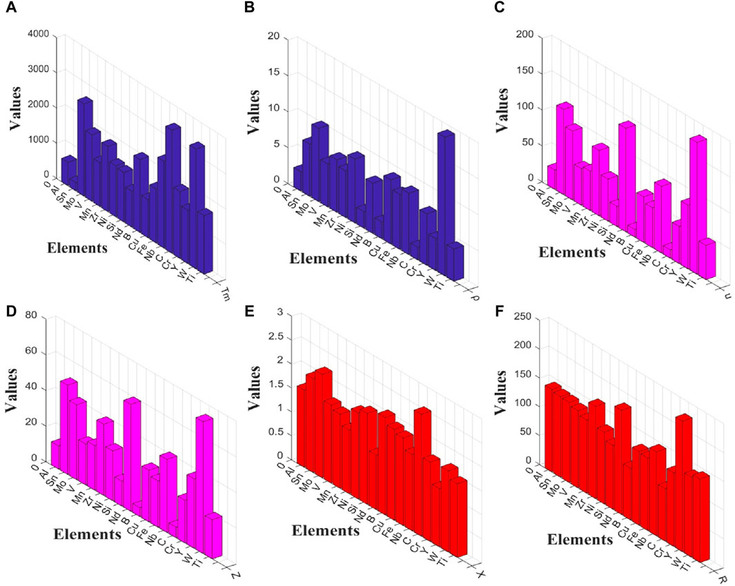
Figure 1. Distribution of physical property constants in titanium alloy: (A) Tm; (B) $\mathrm{\rho }$; (C) u; (D) Z; (E) X; (F) R.

Through the process of original data collection and feature design, the dataset consists of a total of 28 features, that is, 28-dimensional. The detailed information about these features is presented in Table 1.

Table 1

Table 1. Dataset features.

2.1.3 Process of feature selection

In this study, feature selection encompasses both supervised and unsupervised analysis. Within the realm of unsupervised analysis, feature correlation analysis is employed to calculate the correlation coefficients between any given features X and Y, as depicted in Formula 7.

${\mathrm{r}}_{\mathrm{X},\mathrm{Y}}=\frac{\text{Cov}\left(\mathrm{X},\mathrm{Y}\right)}{\sqrt{\mathrm{D}\left(\mathrm{X}\right)}\times \sqrt{\mathrm{D}\left(\mathrm{Y}\right)}}(7)$

Where Cov (X,Y) denotes the covariance between features X and Y, D(X) represents the variance of feature X, and D(Y) represents the variance of feature Y.

In the supervised analysis, the Minimum Redundancy Maximum Relevance (MRMR) algorithm is employed to compute the mutual information between the feature set and ultimate strength, quantifying feature correlation and ranking them accordingly (Peng et al., 2005). For comprehensive selection in the final feature choice, both supervised and unsupervised analysis outcomes are utilized with model accuracy as the target.

2.1.4 Standardization of data

Features originate from diverse scales and encompass multiple dimensions in the dataset. To mitigate the influence of dimensionality, data necessitates processing. Data processing techniques are commonly categorized into normalization and standardization. In engineering applications, standardization is typically preferred. Within this dataset, the data without heat treatment is imputed with zeros. When normalization is performed [0,1], the feature with heat treatment would be skewed towards extreme values of 1 and 0, failing to accurately represent the overall distribution of samples in the data set. Henceforth, standardization is selected as a data processing approach, such as employing Formula 8, which centers the dataset around a mean value of 0 while maintaining a normal distribution with a standard deviation of 1.

$\mathrm{Z}=\frac{\mathrm{C}-\mathrm{\mu }}{\mathrm{\sigma }}(8)$

The feature vector Z is represented as the standardized version of the original arbitrary feature vector C, where μ represents the mean value of feature vector C, and σ represents its standard deviation.

2.1.5 Partitioning of the dataset

The dataset in this research is divided into three parts: the training set, the validation set, and the test set. The training set is utilized for model training, while the validation set serves the purpose of model evaluation, hyperparameter tuning, and mitigating overfitting risks. On the other hand, the test set is exclusively employed for model evaluation and testing.

2.2 Machine learning algorithm model

The model was constructed using six machine learning algorithms in this study, namely, support vector machine regression, Gaussian process regression, neural network regression, CART tree regression, boosting tree regression, and random forest regression.

2.2.1 Support vector machine regression

Support vector machine regression (SVR) is a classic machine learning algorithm for regression proposed by Drucker et al., in 1997 (Drucker et al., 1997), and further developed by Smola et al., in 2004, where the theoretical framework and implementation of SVR was presented (Smola and Schölkopf, 2004). Similar to the SVM classification algorithm, the hyperplane used for classification often cannot completely divide the sample space, which can lead to overfitting even if it is possible to achieve complete division. In SVR, an error tolerance interval band ε is defined, and samples within this band are considered correct predictions without loss calculation. By partitioning the sample space D = {(x₁,y₁), (x₂,y₂),… (x_n,y_n)}, SVR aims to find an optimal hyperplane that minimizes the discrepancy between f(x) and y, as shown in Formula 9.

$\mathrm{f}\left(\mathrm{x}\right)={\mathrm{w}}^{\mathrm{T}}\mathrm{x}+\mathrm{b}(9)$

Where w represents the normal vector indicating the direction of the obtained hyperplane, and b denotes the displacement term representing the distance from the original point of the hyperplane, SVR computes the loss between f(x) and y outside the interval band. The regression problem is formulated in Eq. 10.

$\begin{array}{c}\min \\ \mathrm{w},\mathrm{b}\end{array}\frac{1}{2}{‖\mathrm{w}‖}^2+\mathrm{C}{\displaystyle {\sum }_{\mathrm{i}=1}^{\mathrm{n}}}{\mathrm{l}}_{\mathrm{\epsilon }}\left(\mathrm{f}\left({\mathrm{x}}_{\mathrm{i}}\right)-{\mathrm{y}}_{\mathrm{i}}\right)(10)$

The regularization constant C > 0 is utilized to balance the minimization of the normal vector with the minimization of the error, while ${\mathrm{l}}_{\mathrm{\epsilon }}$ denotes the error tolerant interval incorporating ε insensitive loss function as defined in Formula 11.

${\mathrm{l}}_{\mathrm{\epsilon }}\left(\mathrm{z}\right)=\left\{\begin{array}{l}0,\text{if\hspace{0.17em}}\left|\mathrm{z}\right|\le \mathrm{\epsilon }\\ \left|\mathrm{z}\right|-\mathrm{\epsilon },\text{otherwise}\end{array}\right.(11)$

By incorporating relaxation variables, the Lagrange multiplier method, and kernel functions, SVR can be mathematically formulated as Eq. 12.

$\mathrm{f}\left(\mathrm{x}\right)={\displaystyle {\sum }_{\mathrm{i}=1}^{\mathrm{n}}}\left({\widehat{\mathrm{\alpha }}}_{\mathrm{i}}-{\mathrm{\alpha }}_{\mathrm{i}}\right)\mathrm{k}\left({\mathrm{x}}_i,{\mathrm{x}}_{\mathrm{j}}\right)+\mathrm{b}(12)$

Where ${\mathrm{\alpha }}_{\mathrm{i}}$ represents the Lagrange multiplier, the estimate of ${\mathrm{\alpha }}_{\mathrm{i}}$ is denoted as ${\widehat{\mathrm{\alpha }}}_{\mathrm{i}}$, $\mathrm{k}\left({\mathrm{x}}_i,{\mathrm{x}}_{\mathrm{j}}\right)$ denotes the kernel function, which is a fundamental technique in SVR, and refers to the transformation that maps the indivisible features of the original space to a higher-dimensional divisible space. Since the kernel function implicitly defines the feature space, the specific form of feature mapping remains unknown for a given sample space. Therefore, selecting different kernel functions often yields varying performance outcomes for regression models within specific sample spaces; an inappropriate selection may lead to reduced model performance.

The kernel function is considered as a crucial hyperparameter in this research, and the model is optimized by tuning this hyperparameter. Several commonly used kernel functions are selected, including linear, Gaussian, quadratic, and cubic kernels defined in Formulas 13–16. By adjusting these kernel functions, the optimal SVR regression model is identified.

$\mathrm{k}\left({\mathrm{x}}_{\mathrm{i}},{\mathrm{x}}_{\mathrm{j}}\right)={\mathrm{x}}_{\mathrm{i}}^{\mathrm{T}}{\mathrm{x}}_{\mathrm{j}}(13)$

$\mathrm{k}\left({\mathrm{x}}_{\mathrm{i}},{\mathrm{x}}_{\mathrm{j}}\right)=\exp \left(-\frac{{‖{\mathrm{x}}_{\mathrm{i}}-{\mathrm{x}}_{\mathrm{j}}‖}^2}{2{\mathrm{\sigma }}^2}\right)(14)$

$\mathrm{k}\left({\mathrm{x}}_{\mathrm{i}},{\mathrm{x}}_{\mathrm{j}}\right)={\left({\mathrm{x}}_{\mathrm{i}}^{\mathrm{T}}{\mathrm{x}}_{\mathrm{j}}\right)}^2(15)$

$\mathrm{k}\left({\mathrm{x}}_{\mathrm{i}},{\mathrm{x}}_{\mathrm{j}}\right)={\left({\mathrm{x}}_{\mathrm{i}}^{\mathrm{T}}{\mathrm{x}}_{\mathrm{j}}\right)}^3(16)$

2.2.2 Gaussian process regression

Gaussian process regression (GPR) is a Bayesian non-parametric probabilistic regression model that utilizes a kernel function. The application of Gaussian processes for data fitting was first introduced by O’Hagan in 1978 (OHagan, 1978). Rasmussen et al. (2005) provided a comprehensive theoretical framework for the Gaussian process regression model in machine learning in 2006. The problem of nonlinear Gaussian regression is formulated using Eq. 17.

$\mathrm{y}=\mathrm{f}\left(\mathrm{x}\right)+\mathrm{\epsilon }(17)$

Where ε represents the additive noise term, ε ∼ (0, ${\mathrm{\sigma }}^2$), where ${\mathrm{\sigma }}^2$ can be estimated from the sample data. The variable y denotes the predicted value corrupted by noise, while f(x) follows a Gaussian distribution as described in Eq. 18.

$\mathrm{f}\left(\mathrm{x}\right)\sim \text{GP}\left(\mathrm{m}\left(\mathrm{x}\right),\mathrm{k}\left(\mathrm{x},{\mathrm{x}}^{\prime }\right)\right)(18)$

Where m(x) represents the mean function and takes the value 0. The covariance function k(x,x’) captures the relationship between two features x and x’. In this regression model, Bayesian and maximum likelihood estimation methods are employed to solve for optimal parameters.

The covariance function, denoted as k(x,x’), plays a pivotal role in the model and significantly influences its performance. It is also referred to as the kernel function k(x,x’). In this study, the kernel function is treat as a hyperparameter and optimize the model by adjusting five different types of kernels: quadratic rational (Formula 19), square exponent (Formula 20), Matern 5/2 (Formula 21), Matern 3/2 (Formula 22), and exponent (Formula 23).

$\mathrm{k}\left(\mathrm{x},{\mathrm{x}}^{\prime }\right)={\mathrm{\sigma }}_{\mathrm{f}}^2\left[1+{\left(\frac{{\left(\mathrm{x}-{\mathrm{x}}^{\prime }\right)}^{\mathrm{T}}\left(\mathrm{x}-{\mathrm{x}}^{\prime }\right)}{2\mathrm{\alpha }{\mathrm{l}}^2}\right)}^{-\mathrm{\alpha }}\right](19)$

The symbol α denotes the scaling coefficient, ${\mathrm{\sigma }}_{\mathrm{f}}$ represents the standard deviation of the sample, and l signifies the size of the feature length.

$\mathrm{k}\left(\mathrm{x},{\mathrm{x}}^{\prime }\right)={\mathrm{\sigma }}_{\mathrm{f}}^2\exp \left[-\frac{1}{2}\frac{{\left(\mathrm{x}-{\mathrm{x}}^{\prime }\right)}^{\mathrm{T}}\left(\mathrm{x}-{\mathrm{x}}^{\prime }\right)}{{\mathrm{l}}^2}\right](20)$

$\begin{array}{l}\mathrm{k}\left(\mathrm{x},{\mathrm{x}}^{\prime }\right)={\mathrm{\sigma }}_{\mathrm{f}}^2\left(1+\frac{\sqrt{5{\left(\mathrm{x}-{\mathrm{x}}^{\prime }\right)}^{\mathrm{T}}\left(\mathrm{x}-{\mathrm{x}}^{\prime }\right)}}{\mathrm{l}}+\frac{{5\left(\mathrm{x}-{\mathrm{x}}^{\prime }\right)}^{\mathrm{T}}\left(\mathrm{x}-{\mathrm{x}}^{\prime }\right)}{3{\mathrm{l}}^2}\right)\\ \hfill \exp \left(-\frac{\sqrt{5{\left(\mathrm{x}-{\mathrm{x}}^{\prime }\right)}^{\mathrm{T}}\left(\mathrm{x}-{\mathrm{x}}^{\prime }\right)}}{\mathrm{l}}\right)\left(21\right)\hfill \end{array}$

$\mathrm{k}\left(\mathrm{x},{\mathrm{x}}^{\prime }\right)={\mathrm{\sigma }}_{\mathrm{f}}^2\left(1+\frac{\sqrt{3{\left(\mathrm{x}-{\mathrm{x}}^{\prime }\right)}^{\mathrm{T}}\left(\mathrm{x}-{\mathrm{x}}^{\prime }\right)}}{\mathrm{l}}\right)\exp \left(-\frac{\sqrt{3{\left(\mathrm{x}-{\mathrm{x}}^{\prime }\right)}^{\mathrm{T}}\left(\mathrm{x}-{\mathrm{x}}^{\prime }\right)}}{\mathrm{l}}\right)(22)$

$\mathrm{k}\left(\mathrm{x},{\mathrm{x}}^{\prime }\right)={\mathrm{\sigma }}_{\mathrm{f}}^2\exp \left[-\frac{\sqrt{{\left(\mathrm{x}-{\mathrm{x}}^{\prime }\right)}^{\mathrm{T}}\left(\mathrm{x}-{\mathrm{x}}^{\prime }\right)}}{\mathrm{l}}\right](23)$

2.2.3 Neural network regression

The artificial neural network is a network formed by connecting artificial neurons according to a specific topology, which originated from the MP model proposed by McCulloch et al., in 1943 (McCulloch and Pitts, 1943), as well as the perceptron neural network model introduced by Rosenblatt in 1958 (Rosenblatt, 1958). These models marked the beginning of the development boom for artificial neural networks. However, it was proven in 1969 that perceptrons were incapable of solving higher-order predicates, such as the XOR problem (Minsky et al., 1969). Consequently, the field of artificial neural networks experienced a decline until Hopfield’s proposal of the Hopfield neural network model in 1982 and Rumelhart et al.’s introduction of the BP algorithm in 1986 (Hopfield, 1982; Mcclelland et al., 1986; Rumelhart et al., 1986), which sparked a research upsurge. In this study, a backpropagation (BP) neural network is employed for regression (NNR), where each neuron’s threshold was set as θ = (θ₁, θ₂,… θ_m). Here, m represents the number of non-input layer neurons within the neural network structure. The current output Y_j of neuron j is expressed using Formula 24.

${\mathrm{Y}}_{\mathrm{j}}=\mathrm{f}\left({\displaystyle {\sum }_{\mathrm{i}=1}^{\mathrm{k}}}{\mathrm{w}}_{\text{ij}}{\mathrm{X}}_{\mathrm{i}}-{\mathrm{\theta }}_{\mathrm{j}}\right)(24)$

Where f is the activation function, i=(1,2, … k), j=(1,2, … ,m). The value of k corresponds to the number of neurons located above the current neuron j. The weight w_ij denotes the synaptic connection strength from the ith neuron in the preceding layer to the jth neuron, X_i represents the output value of the ith neuron in the preceding layer, and θ_j signifies the activation threshold of the current neuron.

The weights and thresholds of the BP neural network are iteratively calculated and updated using the gradient descent strategy, leading to the attainment of optimal model values. In this study, the neural network regression model is empirically defined as depicted in Figure 2A, comprising one input layer, one output layer, and three hidden layers. The input layer consists of 28 neurons, while the output layer comprises a single neuron; each hidden layer encompasses 10 neurons.

Figure 2

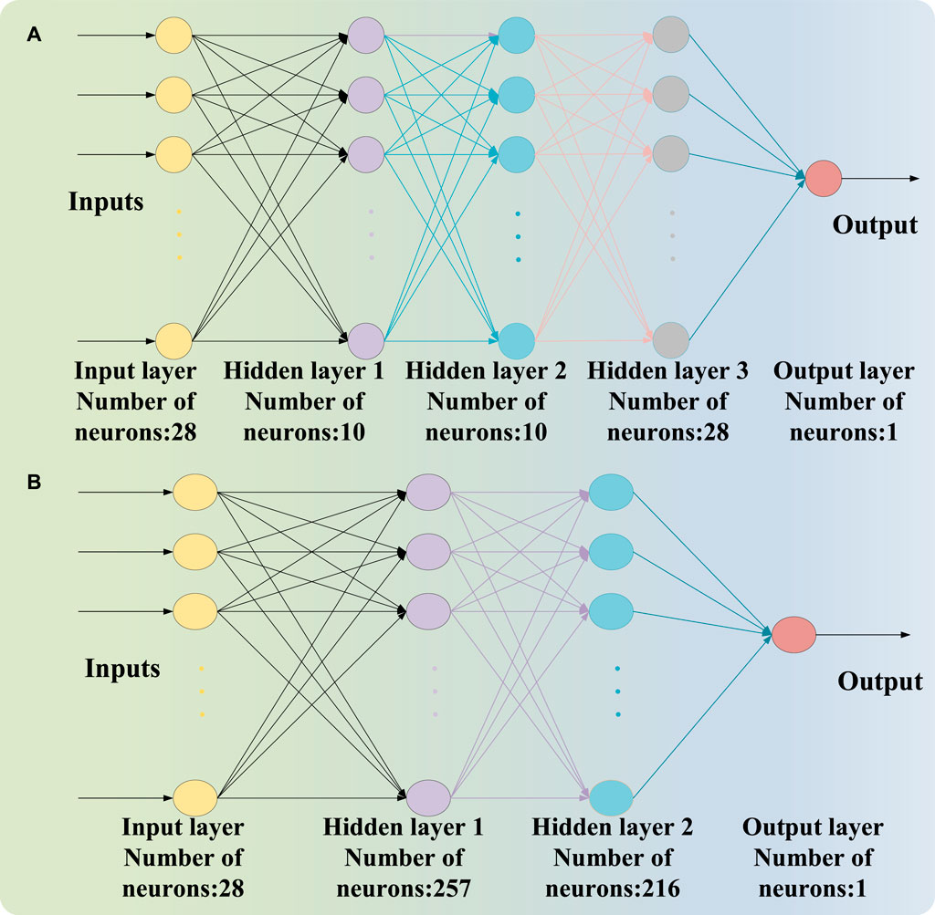
Figure 2. The neural network regression model structure: (A) the neural network regression model based on experience; (B) the neural network regression model based on hyperparameter optimization.

The neural network regression model encompasses numerous crucial hyperparameters, which are devised based on empirical knowledge that may not be deemed as ideal or relatively optimal. Hence, the optimal hyperparameters are fine-tuned by adjusting the parameters of the neural network model and iterating through Bayesian optimization to minimize mean squared error. The range for parameter adjustment is presented in Table 2. The regularization intensity value of 378 corresponds to the aggregate number of training and validation samples.

Table 2

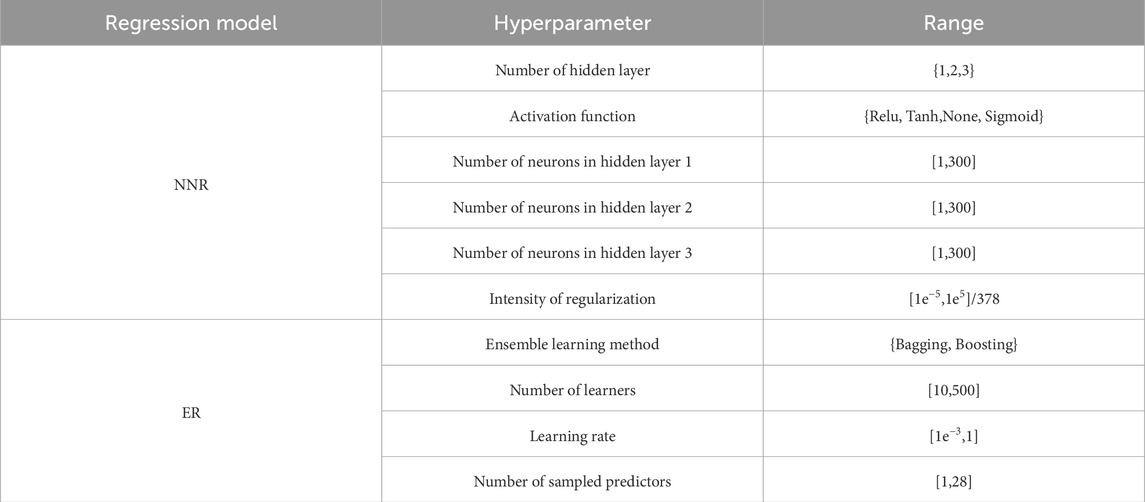
Table 2. The range of hyperparameter optimization.

2.2.4 CART regression

The CART algorithm, proposed by Breiman et al., in 1984 (Breiman et al., 1984), is a classic machine learning algorithm. It comprises two processes: the generation of decision trees and the pruning of decision trees. In the sample feature space, the data is divided into M units (R₁, R₂, … R_M), where each unit i has an output value defined as c_i. The regression tree model is represented by Formula 25.

$\mathrm{f}\left(\mathrm{x}\right)={\displaystyle {\sum }_{\mathrm{i}=1}^{\mathrm{M}}}{\mathrm{c}}_{\mathrm{i}}\mathrm{I}\left(\mathrm{x}\in {\mathrm{R}}_{\mathrm{i}}\right)(25)$

Where I(x∈R_i) represents the adaptation function for spatial feature partitioning, which is optimized by minimizing the square error and determining the optimal output value of each partition unit as the average of all observed values. The optimal feature j and segmentation point s on the partitioned feature are solved using Formula 26.

$\underset{\mathrm{j},\mathrm{s}}{\min }\left[\underset{{\mathrm{c}}_1}{\min }{\displaystyle {\sum }_{{\mathrm{x}}_{\mathrm{i}}\in {\mathrm{R}}_1\left(\mathrm{j},\mathrm{s}\right)}}{\left({\mathrm{y}}_{\mathrm{i}}-{\mathrm{c}}_1\right)}^2+\underset{{\mathrm{c}}_2}{\min }{\displaystyle {\sum }_{{\mathrm{x}}_2\in {\mathrm{R}}_2\left(\mathrm{j},\mathrm{s}\right)}}{\left({\mathrm{y}}_{\mathrm{i}}-{\mathrm{c}}_2\right)}^2\right](26)$

The optimal value of c₁ in R₁ is indicated by Formula 27, while the optimal value of c₂ in R₂ is denoted by Formula 28.

${\widehat{\mathrm{c}}}_1=\text{ave}\left({\mathrm{y}}_{\mathrm{i}}|{\mathrm{x}}_{\mathrm{i}}\in {\mathrm{R}}_1\left(\mathrm{j},\mathrm{s}\right)\right)(27)$

${\widehat{\mathrm{c}}}_2=\text{ave}\left({\mathrm{y}}_{\mathrm{i}}|{\mathrm{x}}_{\mathrm{i}}\in {\mathrm{R}}_2\left(\mathrm{j},\mathrm{s}\right)\right)(28)$

By evaluating the loss function, pruning is performed iteratively from the leaf nodes to the root node of the generated decision tree. The pruned subtree, denoted as {T₀,T₁, … T_k}, is determined based on a calculated subtree loss function using Formula 29.

${\mathrm{C}}_{\mathrm{\alpha }}\left(\mathrm{T}\right)=\mathrm{C}\left(\mathrm{T}\right)+\mathrm{\alpha }\left|\mathrm{T}\right|(29)$

The cost of pruning, denoted as C(T), is the square error associated with any subtree T, while |T| represents the complexity of the model in terms of the number of leaf nodes. Here, α is a weight parameter that balances model fitting and complexity, ultimately determining the generalization ability of the model.

In this study, the termination condition of the CART algorithm was defined as the minimum leaf size, which represents the number of samples in a leaf node. Initially, this value is set to 12 based on empirical knowledge for model regression. However, it is important to note that this initial setting may not be optimal or ideal. The hyperparameter for the minimum leaf size of the CART regression model was adjusted accordingly. Bayesian optimization and iterative processes were employed to optimize the hyperparameter based on minimizing mean squared error. Consequently, the minimum leaf size was set to [1,378/2].

2.2.5 Ensemble tree regression

The Boosting tree algorithm, proposed by Friedman et al., in 2000 (Friedman et al., 2000), is considered one of the most high-performing ensemble learning algorithms. Boosting tree is an ensemble algorithm based on decision trees and utilizes a boosting technique that employs additive models and forward distribution algorithms, following a sequential approach. The weak learners are combined into strong learners by linearly combining basis functions with weights. In this boosting tree regression model, which uses the CART algorithm as the basis function, which is defined by Formula 30.

${\mathrm{f}}_{\mathrm{M}}\left(\mathrm{x}\right)={\displaystyle {\sum }_{\mathrm{m}=1}^{\mathrm{M}}}\mathrm{T}\left(\mathrm{x},{\mathrm{\Theta }}_{\mathrm{m}}\right)(30)$

Where T(x,Θ) is the decision tree generated by CART algorithm. M represents the number of decision trees and Θ_m represents the weight of the mth decision tree. The current model of the boosting tree is defined as f_(m-1)(x), and thus, Formula 31 illustrates the weight of the mth decision tree.

${\widehat{\mathrm{\Theta }}}_{\mathrm{m}}=\arg \underset{{\mathrm{\Theta }}_{\mathrm{m}}}{\min }{\displaystyle {\sum }_{\mathrm{i}=1}^{\mathrm{N}}}\mathrm{L}\left({\mathrm{y}}_{\mathrm{i}},\mathrm{\eta }\left({\mathrm{f}}_{\mathrm{m}-1}\left({\mathrm{x}}_{\mathrm{i}}\right)+\mathrm{T}\left({\mathrm{x}}_{\mathrm{i}};{\mathrm{\Theta }}_{\mathrm{m}}\right)\right)\right)(31)$

The loss function is defined as the mean squared error, and the optimal weight corresponds to the weight that minimizes the mean squared error. Here, η denotes the learning rate. The boosting tree model involves several crucial hyperparameters. Based on empirical knowledge, the minimum leaf node is set to be 8, with a total of 30 learners and a learning rate of 0.1 for boosting tree regression.

Random forest, proposed by Breiman in 2001 (Breiman, 2001), is a bagging ensemble algorithm based on decision trees. Bagging involves generating multiple decision trees by randomly selecting and replacing feature and sample sets, and the predicted values of all decision trees are averaged during prediction, thereby parallelly combining the basis functions. In this random forest regression model, the CART algorithm is employed as the basis function and consider several important hyperparameters. Based on empirical knowledge, the minimum leaf node hyperparameter is set to 8 and use 30 learners for random forest regression.

However, the empirical values in the regression models of the boosting tree and random forest may not be inherently optimal or ideal. The hyperparameters of the model were adjusted and iterated using Bayesian optimization to optimize the optimal hyperparameters, based on the minimum mean squared error. The range of hyperparameter adjustments is presented in Table 2.

2.3 Model evaluation

In this study, five methods were employed to assess the machine learning regression model: root mean squared error (RMSE), mean absolute error (MAE), coefficient of determination (R²), mean squared error (MSE), and training time (T).

2.3.1 Root mean squared error

The root mean squared error is a widely used metric for evaluating regression models, which quantifies the average degree of deviation between predicted and true values as expressed in Formula 32.

$\text{RMSE}=\sqrt{\frac{{\displaystyle {\sum }_{\mathrm{i}=1}^{\mathrm{n}}}{\left({\mathrm{y}}_{\mathrm{i}}-{\widehat{\mathrm{y}}}_{\mathrm{i}}\right)}^2}{\mathrm{n}}}(32)$

Where n denotes the number of samples, y_i represents the ith true value to be predicted, and ${\widehat{\mathrm{y}}}_{\mathrm{i}}$ denotes the ith predicted value. The formula reveals that a smaller RMSE value indicates a closer proximity between the predicted and true values, thereby signifying an enhanced fitting degree and performance of the regression model.

2.3.2 Mean absolute error

The mean absolute error is a commonly employed metric for evaluating regression models, quantifying the mean discrepancy between predicted and true values as defined in Eq. 33.

$\text{MAE}=\frac{{\displaystyle {\sum }_{\mathrm{i}=1}^{\mathrm{n}}}\left|{\mathrm{y}}_{\mathrm{i}}-{\widehat{\mathrm{y}}}_{\mathrm{i}}\right|}{\mathrm{n}}(33)$

The formula reveals that a smaller MAE value corresponds to a narrower discrepancy between the predicted and true values, indicating an enhanced level of fitting and performance for the regression model.

2.3.3 Coefficient of determination

The coefficient of determination, a crucial evaluation index of regression models, quantifies the correlation between dependent and independent variables while representing the explanatory power of the regression model for the dependent variable. The calculation is presented in Formula 34.

${\mathrm{R}}^2=1-\frac{\text{SSE}}{\text{SST}}=1-\frac{{\displaystyle {\sum }_{\mathrm{i}=1}^{\mathrm{n}}}{\left({\mathrm{y}}_{\mathrm{i}}-{\widehat{\mathrm{y}}}_{\mathrm{i}}\right)}^2}{{\displaystyle {\sum }_{\mathrm{i}=1}^{\mathrm{n}}}{\left({\mathrm{y}}_{\mathrm{i}}-\mathrm{\mu }\right)}^2}(34)$

The sum of squares of error (SSE) represents the discrepancy between the predicted values and the true values in the model. On the other hand, the total sum of squares (SST) represents the overall deviation between all predicted true values and their mean value. Here, μ denotes the average value of all true values. It is evident from this formula that R² typically ranges between 0 and 1, indicating a prediction error lower than that of mean reference. As R² approaches 1, it signifies a higher goodness-of-fit for the regression model, implying superior performance. Conversely, when R² is negative, it suggests poor predictive ability and greater prediction errors compared to mean reference.

2.3.4 Mean squared error

The mean squared error is a widely used metric for evaluating regression models, quantifying the discrepancy between predicted and true values as computed in Formula 35.

$\text{MSE}=\frac{{\displaystyle {\sum }_{\mathrm{i}=1}^{\mathrm{n}}}{\left({\mathrm{y}}_{\mathrm{i}}-{\widehat{\mathrm{y}}}_{\mathrm{i}}\right)}^2}{\mathrm{n}}(35)$

The formula reveals that a smaller MSE value corresponds to a closer proximity between the predicted and true values, indicating an enhanced level of fitting and performance for the regression model.

2.3.5 Training time

The training time reflects the model’s complexity and encompasses the time taken from the initiation to completion of training. On a consistent hardware platform, shorter training times indicate higher efficiency in model learning. For models with substantial time requirements, the training time serves as a crucial evaluation metric.

2.4 Model selection

Given this emphasis on model prediction accuracy, the training time serves as a mere reference, while the optimal model is selected based on various hyperparameter optimized models using RMSE, MAE, R², and MSE.

3 Results and discussion

The experiment was conducted using MATLAB software. To enhance the model’s generalization ability, the training set and validation set were obtained through a ten-fold cross-validation approach, where 5% of the dataset (19 samples) was randomly selected for testing purposes while the remaining 95% (378 samples) was divided into training and validation sets.

3.1 Feature engineering based on titanium alloys

3.1.1 Feature selection

The unsupervised feature correlation coefficient results are presented in Figure 3A. It is evident that features Z and u, as well as X and Cr, exhibit a relatively high degree of correlation with correlation coefficients exceeding 0.9, which is a correlation threshold of experience.

Figure 3

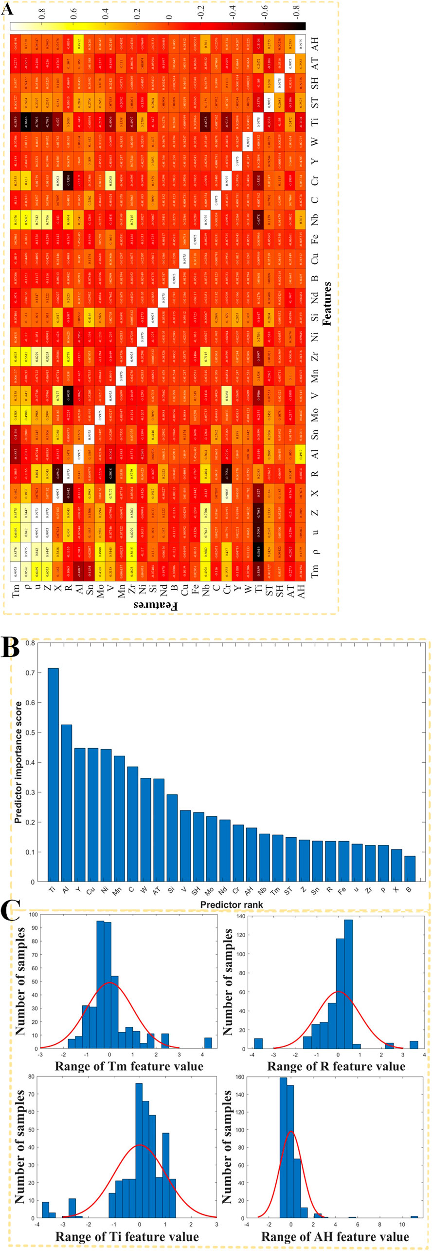
Figure 3. Feature engineering based on titanium alloys: (A) heat map of unsupervised feature correlation coefficients; (B) ranking of feature correlation under supervision; (C) histogram of normalized features.

The ranking results of feature correlation based on the supervised MRMR algorithm are presented in Figures 3A, B comprehensive analysis is conducted by considering the features associated with the supervised comparison. Specifically, Z exhibits a feature correlation score of 0.1395, u has a score of 0.1270, X is assigned a score of 0.1083, and Cr demonstrates a score of 0.1899. These features are all evaluated as significant contributors to the model’s performance. In order to construct a high-precision prediction model, all 28 features are retained without any exclusion.

3.1.2 Standardization of data

After standardization, the data for each of the 28 features conforms to a normal distribution with a mean value of 0 and a standard deviation of 1, a random selection of 4 features was made to construct the histogram, as illustrated in Figure 3C.

3.2 Machine learning algorithm model

3.2.1 Support vector machine regression

In the support vector machine regression model, the hyperparameters were optimized to include linear, Gaussian, quadratic and cubic kernel functions. The resulting performance metrics including RMSE, MAE, R² and MSE as well as training time T are presented in Table 3.

Table 3

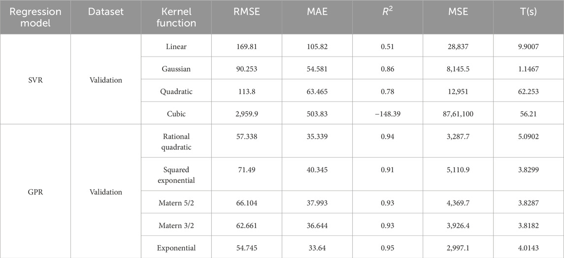
Table 3. Optimization outcomes of hyperparameters for SVR and GPR models.

The optimal hyperparameter of the model is determined to be the Gaussian kernel function, as evidenced by the smallest values of RMSE, MAE, and MSE, along with an R² value of 0.86 (Table 3). The model performance is unsatisfactory when the hyperparameter selects the cubic kernel function, as indicated by an R² value of −148.39, which exceeds the mean reference error and indicates poor prediction accuracy. Figure 4A illustrates the comparison between real and predicted values for this particular response.

Figure 4

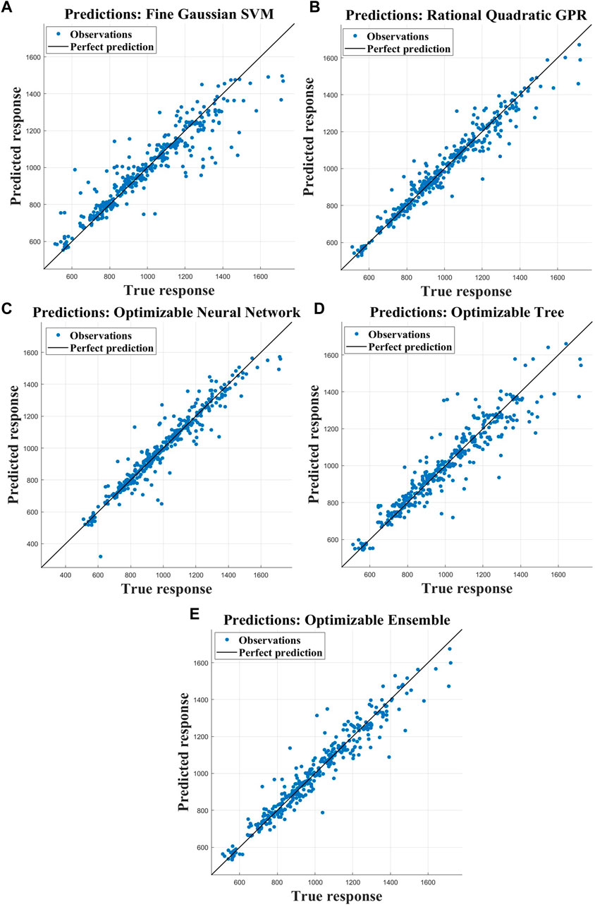
Figure 4. The response of the true value and predicted value of the model following hyperparameter optimization: (A) SVR; (B) GPR; (C) NNR; (D) CART; (E) ER.

3.2.2 Gaussian process regression

In the Gaussian process regression model, the hyperparameters of the model were adjusted to incorporate rational quadratic, squared exponential, Matern 5/2, Matern 3/2, and exponential kernel functions. The performance metrics including RMSE, MAE, R², MSE, and training time T were presented in Table 3.

The optimal hyperparameter of the model is determined to be the exponential kernel function, as evidenced by the smallest values of RMSE, MAE, and MSE, along with an impressive R² value of 0.95 (Table 3). The corresponding responses between real and predicted values are visually depicted in Figure 4B.

3.2.3 Neural network regression

The results of the neural network regression, including RMSE, MAE, R², MSE, and training time T, are presented in Table 4. Additionally, Figure 5A illustrates the iterative outcomes of the hyperparameter optimization algorithm. It is evident from the figure that convergence occurs during the third iteration and yields optimized hyperparameters as follows: two hidden layers with a Tanh activation function; 257 neurons in hidden layer 1 and 216 neurons in hidden layer 2; Intensity of regularization set at 0.2791. The optimized neural network regression model is depicted in Figure 2B.

Table 4

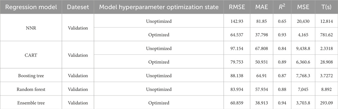
Table 4. Optimization outcomes of hyperparameters for NNR, CART, Boosting tree, Random forest and Ensemble tree models.

Figure 5

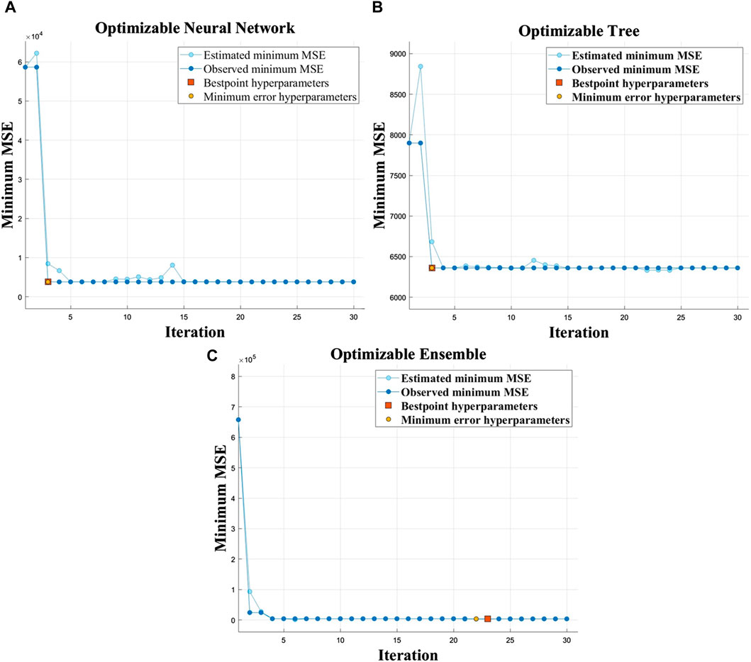
Figure 5. Iteration for optimizing model hyperparameters: (A) NNR; (B) CART; (C) ER.

The optimized NNR model has exhibited significant performance enhancement, as evident from the results presented in Table 4. Notably, there has been a substantial reduction in the values of RMSE, MAE, and MSE, while R² has increased from 0.65 to 0.93. Figure 4C illustrates the comparison between actual and predicted values.

3.2.4 CART regression

The performance evaluation of CART tree regression models, including RMSE, MAE, R², MSE and training time T, is presented in Table 4. The iterative results of the hyperparameter optimization algorithm are illustrated in Figure 5B. It can be observed from the figure that the algorithm achieves convergence after three iterations with optimized hyperparameters: a minimum leaf size of 2.

The optimization of the model has led to a noticeable improvement in performance, as evident from the data presented in Table 4. Specifically, there has been a reduction in RMSE, MAE, and MSE values, indicating enhanced accuracy. Moreover, the R² value has increased significantly from 0.84 to 0.89. Figure 4D illustrates the correlation between actual and predicted values.

3.2.5 Ensemble tree regression

The performance metrics, including RMSE, MAE, R², MSE, and training time T of the boosting tree and random forest regression models in the ensemble tree regression approach are presented in Table 4. The iterative results of the hyperparameter optimization algorithm are illustrated in Figure 5C. It can be observed from the figure that the algorithm converges at the 23rd iteration with optimized hyperparameters as follows: Boosting algorithm is employed for ensemble learning method with a total of 497 learners, minimum leaf size set to 7, learning rate set to 0.0675, and number of sampled predictors limited to 5.

The performance of the empirically defined random forest regression model is superior to that of the boosting tree regression model, as evident from Table 4 prior to hyperparameter optimization. Moreover, the random forest regression model exhibits smaller values for RMSE, MAE, and MSE compared to the boosting tree regression model. Additionally, the R² value of the random forest regression model surpasses that of the boosting tree regression model by 0.01. Subsequent optimization resulted in decreased RMSE, MAE, and MSE values along with an increased R² value of 0.94, leading to a more refined and optimized model. Figure 4E illustrates the comparison between real and predicted values.

3.3 Model selection

The optimized Gaussian regression model with exponential hyperparameter exhibits superior performance compared to all other models, as evident from the results presented in Tables 3, 4. It achieves a lower RMSE of 54.745, MAE of 33.64, and MSE of 2997.1, outperforming the other optimized models. Additionally, it attains an impressive R² value of 0.95 surpasses existing literature benchmarks (refer to Table 5 for detailed comparisons). This enhancement can be primarily attributed to this meticulous feature engineering and comprehensive model optimization based on titanium alloys.

Table 5

Table 5. The comparison of model R².

In order to validate this model, model verification was conducted on the test set. The RMSE of the model on the test set was 68.53, with an MAE of 42.239, MSE of 4696.3, and R² value of 0.93, indicating excellent performance. Table 6 presents the prediction results obtained from the optimized Gaussian regression model applied to the test set. Figure 6A illustrates both true and predicted responses, while Figure 6B displays the residuals.

Table 6

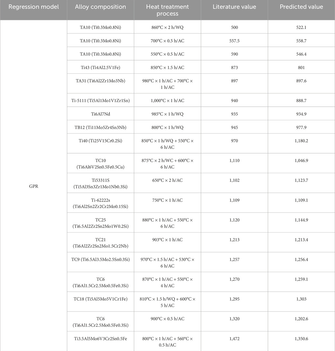
Table 6. Comparison of predicted and literature values on the test set.

Figure 6

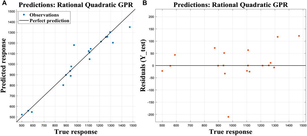
Figure 6. Predict results on the test set: (A) response of true value and predicted value; (B) residual of true value.

3.4 Comprehensive model framework

The present study introduces a comprehensive computer-aided design framework for high-performance titanium alloys based on machine learning, as depicted in Figure 7. This framework comprises three main components: feature engineering based on titanium alloys, machine learning algorithm model, and model evaluation and selection. By utilizing the proposed model, it becomes possible to generate any titanium alloy sequence based on the input of titanium and predict its ultimate strength using the established model architecture. Consequently, the output will provide the optimal titanium alloy sequence with superior ultimate strength properties, thereby facilitating the design process of high-performance titanium alloys. Moreover, this model also demonstrates capability in predicting the properties of heat-treated titanium alloys. In theory, the proposed model has unlimited potential to predict ultimate strength properties for all conceivable combinations of titanium based on 18 elements. From a broader perspective, this represents an inexhaustible search for novel materials in the field of titanium alloy design. For the purpose of this illustration the designed Ti6Al4Vx₁Six₂Mox₃Snx₄Nd series titanium alloy was subjected to computer aided high-performance design using the proposed framework, with x₁, x₂, x₃, and x₄ limited to a value range of [0.1,5] and a step size of 0.1. A total of 6250,000 combinations were generated. Among all combinations, Ti6Al4V0.3Si5Mo2.3Sn0.1Nd exhibited the most optimal performance with an ultimate strength of 1,139.9 MPa.

Figure 7

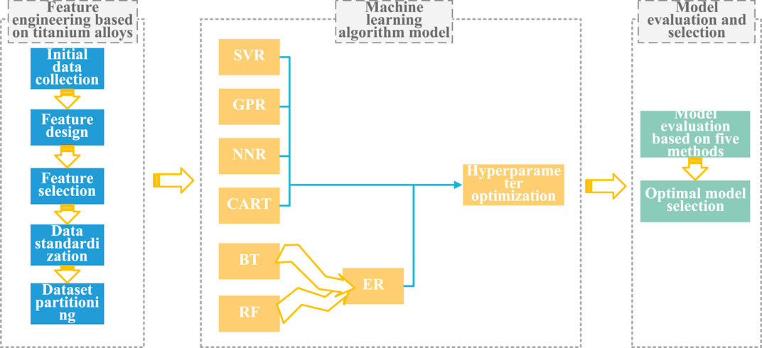
Figure 7. Comprehensive model framework.

4 Conclusion

In this study, a computer-aided framework for designing high-performance titanium alloys based on machine learning techniques and an intelligent search space driven by data to facilitate the design process have been proposed. The main results are summarized as follows:

(1) In the feature engineering based on titanium alloy, the data are sourced exclusively from literature, ensuring an open and comprehensive data acquisition process. This approach enables a more universal and accessible dataset. Six essential properties of titanium alloy were meticulously designed to avoid any dimensionality issues. For feature selection, both supervised and unsupervised analysis was conducted, resulting in the establishment of a proprietary dataset for titanium alloy comprising 397 data samples and 28 features.

(2) The machine learning algorithm model incorporates six classical regression algorithms to construct the model, and hyperparameter optimization is employed to enhance its performance.

(3) The model evaluation and selection process involved the utilization of five regression model evaluation methods, ultimately leading to the identification of the optimal Gaussian regression model with an impressive R² value of 0.95. This achievement signifies a higher level of technical proficiency. Furthermore, the performance of the model on an independent test set has been validated, which yielded a satisfactory prediction result with an R² value of 0.93.

(4) A comprehensive machine learning framework has been proposed, and a model for high-performance titanium alloys has been established. In essence, this model represents an exhaustive intelligent search capable of exploring titanium alloys that incorporate any combination of the remaining 18 elements. Furthermore, the proposed framework is utilized to present a predictive model for a novel titanium alloy, Ti6Al4V0.3Si5Mo2.3Sn0.1Nd, with an ultimate strength of 1,139.9 MPa.

In future research, the investigation on laser powder bed fusion additive manufacturing of high performance titanium alloys with the proposed framework was conducted, encompassing the examination of printing process parameters and heat treatment effects on microstructure and mechanical properties.

Data availability statement

The raw data supporting the conclusion of this article will be made available by the authors, without undue reservation.

Author contributions

SA: Investigation, Methodology, Writing–original draft, Writing–review and editing. KL: Writing–original draft. LZ: Investigation, Writing–review and editing. HL: Investigation, Writing–review and editing. RM: Investigation, Writing–review and editing. RL: Investigation, Methodology, Writing–review and editing. LM: Investigation, Methodology, Writing–review and editing.

Funding

The author(s) declare that no financial support was received for the research, authorship, and/or publication of this article.

Acknowledgments

The authors gratefully acknowledge all the researchers and labs to provide the experimental facilities. KL acknowledges the support from National Natural Science Foundation of China (52201105), Natural Science Foundation of Chongqing (CSTB2022NSCQ-MSX0992), Innovation Support Program for Overseas Returnees in Chongqing (cx2023061), Research, Natural Science Foundation of Sichuan Province (2023NSFSC0407).

Conflict of interest

Author SA was employed by AVIC Guizhou Aircraft Corporation LTD.

The remaining authors declare that the research was conducted in the absence of any commercial or financial relationships that could be construed as a potential conflict of interest.

Publisher’s note

All claims expressed in this article are solely those of the authors and do not necessarily represent those of their affiliated organizations, or those of the publisher, the editors and the reviewers. Any product that may be evaluated in this article, or claim that may be made by its manufacturer, is not guaranteed or endorsed by the publisher.

Supplementary material

The Supplementary Material for this article can be found online at: https://www.frontiersin.org/articles/10.3389/fmats.2024.1364572/full#supplementary-material

References

Boyer, R. R. (1995). Titanium for aerospace: rationale and applications. Adv. Perform. Mater. 2, 349–368. doi:10.1007/bf00705316

CrossRef Full Text | Google Scholar

Breiman, L. (2001). Random forests. Mach. Learn. 45, 5–32. doi:10.1023/a:1010933404324

CrossRef Full Text | Google Scholar

Breiman, L., Friedman, J. H., Olshen, R. A., and Stone, C. J. (1984). Classification and regression trees. Boca Raton, FL, USA: Chapman and Hall/CRC.

Google Scholar

Chen, L., and Guantao, L. (2005). The characteristics and application of titanium alloys in ship. Ship Sci. Technol. 27, 13–15.

Google Scholar

Cheng, J., Li, J., Yu, S., Du, Z., Zhang, X., Zhang, W., et al. (2021). Influence of isothermal ω transitional phase-assisted phase transition from β to α on room-temperature mechanical performance of a meta-stable β titanium alloy Ti−10Mo−6Zr−4Sn−3Nb (Ti-B12) for medical application. Front. Bioeng. Biotechnol. 8, 626665. doi:10.3389/fbioe.2020.626665

PubMed Abstract | CrossRef Full Text | Google Scholar

Cheng, J., Yu, S., Li, J., Gai, J., Du, Z., Dong, F., et al. (2022). Precipitation behavior and microstructural evolution of α phase during hot deformation in a novel β-air-cooled metastable β-type Ti-B12 alloy. Metals 12, 770. doi:10.3390/met12050770

CrossRef Full Text | Google Scholar

Deng, Z. H., Yin, H. q., Jiang, X., Zhang, C., Zhang, G. f., Xu, B., et al. (2020). Machine-learning-assisted prediction of the mechanical properties of Cu–Al alloy. Int. J. Minerals. Metallurgy Mater. 3, 362–373. doi:10.1007/s12613-019-1894-6

CrossRef Full Text | Google Scholar

Drucker, H., Burges, C. J. C., Kaufman, L., Kaufman, B. L., Smola, A., Vapnik, V., et al. (1997). “Support vector regression machines,” in Advances in neural information processing systems 9(NIPS) (Cambridge, MA, USA: MIT Press), 155–161.

Google Scholar

Fotovvati, B., and Chou, K. (2022). Build surface study of single-layer raster scanning in selective laser melting: surface roughness prediction using deep learning. Manuf. Lett. 33, 701–711. doi:10.1016/j.mfglet.2022.07.088

CrossRef Full Text | Google Scholar

Friedman, J., Tibshirani, R., and Hastie, T. (2000). Additive logistic regression: a statistical view of boosting (With discussion and a rejoinder by the authors). Ann. Statistics 28, 337–407. doi:10.1214/aos/1016120463

CrossRef Full Text | Google Scholar

Giles, S. A., Sengupta, D., Broderick, S. R., and Rajan, K. (2022). Machine-learning-based intelligent framework for discovering refractory high-entropy alloys with improved high-temperature yield strength. npj Comput. Mater. 8, 235. doi:10.1038/s41524-022-00926-0

CrossRef Full Text | Google Scholar

Guo, Z., Shen, X., Liu, F., Guan, J., Zhang, Y., Dong, F., et al. (2023). Microstructure and mechanical properties of Alx(TiZrTa0.7NbMo) refractory high-entropy alloys. J. Alloys Compd. 960, 170739. doi:10.1016/j.jallcom.2023.170739

CrossRef Full Text | Google Scholar

Hanawa, T. (2019). Overview of metals and applications. Metals for biomedical devices. New Delhi, India: Woodhead Publishing, 3–24.

CrossRef Full Text | Google Scholar

Hopfield, J. J. (1982). Neural networks and physical systems with emergent collective computational abilities. Proc. Natl. Acad. Sci. 79, 2554–2558. doi:10.1073/pnas.79.8.2554

PubMed Abstract | CrossRef Full Text | Google Scholar

Ji, Y. Z., Issa, A., Heo, T., Saal, J., Wolverton, C., and Chen, L. Q. (2014). Predicting β′ precipitate morphology and evolution in Mg–RE alloys using a combination of first-principles calculations and phase-field modeling. Acta Mater. 76, 259–271. doi:10.1016/j.actamat.2014.05.002

CrossRef Full Text | Google Scholar

Jiang, L., Wang, C., Fu, H., Shen, J., Zhang, Z., and Xie, J. (2022). Discovery of aluminum alloys with ultra-strength and high-toughness via a property-oriented design strategy. J. Mater. Sci. Technol. 3, 33–43.

CrossRef Full Text | Google Scholar

Kandavalli, M., Agarwal, A., Poonia, A., Kishor, M., and Ayyagari, K. P. R. (2023). Design of high bulk moduli high entropy alloys using machine learning. Sci. Rep. 13, 20504. doi:10.1038/s41598-023-47181-x

PubMed Abstract | CrossRef Full Text | Google Scholar

Kang, X. D., Du, Z., Wang, Z., Yue, Z., Wang, S., Li, J., et al. (2024). Efficient access to ultrafine crystalline metastable-β titanium alloy via dual-phase recrystallization competition. J. Mater. Res. Technol. 29, 335–343. doi:10.1016/j.jmrt.2024.01.101

CrossRef Full Text | Google Scholar

Li, K., Ma, R., Qin, Y., Gong, N., Wu, J., Wen, P., et al. (2023). A review of the multi-dimensional application of machine learning to improve the integrated intelligence of laser powder bed fusion. J. Mater. Process. Technol. 318, 118032. doi:10.1016/j.jmatprotec.2023.118032

CrossRef Full Text | Google Scholar

Liu, H., Wang, Z., Cheng, J., Li, N., Liang, S. X., Zhang, L., et al. (2023). Nb-content-dependent passivation behavior of Ti–Nb alloys for biomedical applications. J. Mater. Res. Technol. 27, 7882–7894. doi:10.1016/j.jmrt.2023.11.203

CrossRef Full Text | Google Scholar

Liu, Q., Zhang, Z., Liu, S., and Yang, H. (2015). Application and development of titanium alloy in aerospace and military hardware. J. Iron Steel Res. 27, 1–4.

Google Scholar

Liu, S., Song, X., Xue, T., Ma, N., Wang, Y., and Wang, L. (2020). Application and development of titanium alloy and titanium matrix composites in aerospace field. J. Aeronautical Mater. 40, 77–94.

Google Scholar

Lourenço, M. L., Cardoso, G. C., Sousa, K. d. S. J., Donato, T. A. G., Pontes, F. M. L., and Grandini, C. R. (2020). Development of novel Ti-Mo-Mn alloys for biomedical applications. Sci. Rep. 10, 6298–8. doi:10.1038/s41598-020-62865-4

PubMed Abstract | CrossRef Full Text | Google Scholar

Mao, H. H., Chen, H. L., and Chen, Q. (2017). TCHEA1: a thermodynamic database not limited for “high entropy” alloys. J. Phase Equilibria Diffusion 4, 353–368. doi:10.1007/s11669-017-0570-7

CrossRef Full Text | Google Scholar

McClelland, J. L., and Rumelhart, D. E.the PDP Research Group (1986). Parallel distributed processing: explorations in the microstructure of cognition. Psychol. Biol. Models 2.

Google Scholar

McCulloch, W. S., and Pitts, W. (1943). A logical calculus of the ideas immanent in nervous activity. Bull. Math. Biophysics 5, 115–133. doi:10.1007/bf02478259

CrossRef Full Text | Google Scholar

Minsky, M. L., Papert, M., and Seymour, (1969). Perceptrons: an introduction to computational geometry. Cambridge, MA, USA: The MIT Press.

Google Scholar

OHagan, A. (1978). Curve fitting and optimal design for prediction. J. R. Stat. Soc. Ser. B Methodol. 40, 1–24. doi:10.1111/j.2517-6161.1978.tb01643.x

CrossRef Full Text | Google Scholar

Peng, H. C., Fuhui Long, , and Ding, C. (2005). Feature selection based on mutual information: criteria of max-dependency, max-relevance, and min-redundancy. IEEE Trans. Pattern Analysis Mach. Intell. 27, 1226–1238. doi:10.1109/tpami.2005.159

PubMed Abstract | CrossRef Full Text | Google Scholar

Rao, Z. Y., Springer, H., Ponge, D., and Li, Z. (2022a). Combinatorial development of multicomponent invar alloys via rapid alloy prototyping. Materialia 21, 101326. doi:10.1016/j.mtla.2022.101326

CrossRef Full Text | Google Scholar

Rao, Z. Y., Tung, P. Y., Xie, R., Wei, Y., Zhang, H., Ferrari, A., et al. (2022b). Machine learning–enabled high-entropy alloy discovery. Science 378, 78–85. doi:10.1126/science.abo4940

PubMed Abstract | CrossRef Full Text | Google Scholar

Rasmussen, C. E., and Williams, C. K. I. (2005). Gaussian processes for machine learning. Cambridge, MA, USA: MIT Press.

Google Scholar

Ren, F., Ward, L., Williams, T., Laws, K. J., Wolverton, C., Hattrick-Simpers, J., et al. (2018). Accelerated discovery of metallic glasses through iteration of machine learning and high-throughput experiments. Sci. Adv. 4, eaaq1566. doi:10.1126/sciadv.aaq1566

PubMed Abstract | CrossRef Full Text | Google Scholar

Rosenblatt, F. (1958). The perceptron: a probabilistic model for information storage and organization in the brain. Psychol. Rev. 65, 386–408. doi:10.1037/h0042519

PubMed Abstract | CrossRef Full Text | Google Scholar

Rumelhart, D., Hinton, G. E., and Williams, R. J. (1986). Learning representations by back-propagating errors. Nature 323, 533–536. doi:10.1038/323533a0

CrossRef Full Text | Google Scholar

Sarraf, M., Rezvani Ghomi, E., Alipour, S., Ramakrishna, S., and Liana Sukiman, N. (2022). A state-of-the-art review of the fabrication and characteristics of titanium and its alloys for biomedical applications. Bio-design Manuf. 5, 371–395. doi:10.1007/s42242-021-00170-3

CrossRef Full Text | Google Scholar

Sasidhar, K. N., Siboni, N. H., Mianroodi, J. R., Rohwerder, M., Neugebauer, J., and Raabe, D. (2023). Enhancing corrosion-resistant alloy design through natural language processing and deep learning. Sci. Adv. 9, eadg7992. doi:10.1126/sciadv.adg7992

PubMed Abstract | CrossRef Full Text | Google Scholar

Shen, X. Y., Liu, F., Guan, J., Dong, F., Zhang, Y., Guo, Z., et al. (2024). Effect of hydrogen on thermal deformation behavior and microstructure evolution of MoNbHfZrTi refractory high-entropy alloy. Intermetallics. 166, 108193. doi:10.1016/j.intermet.2024.108193

CrossRef Full Text | Google Scholar

Smola, A. J., and Schölkopf, B. (2004). A tutorial on support vector regression. Statistics Comput. 14, 199–222. doi:10.1023/b:stco.0000035301.49549.88

CrossRef Full Text | Google Scholar

Song, D., Niu, L., and Yang, S. (2020). Research on application technology of titanium alloy in marine pipeline. Rare Metal Mater. Eng. 49, 1100–1104.

Google Scholar

Song, X. L., Fu, X., and Wang, M. (2023). First-principles study of β′ phase in Mg-RE alloys. Int. J. Mech. Sci. 243, 108045. doi:10.1016/j.ijmecsci.2022.108045

CrossRef Full Text | Google Scholar

Tian, X. H., Zhou, L., Zhang, K., Zhao, Q., Li, H., Shi, D., et al. (2022). Screening for shape memory alloys with narrow thermal hysteresis using combined XGBoost and DFT calculation. Comput. Mater. Sci. 211, 111519. doi:10.1016/j.commatsci.2022.111519

CrossRef Full Text | Google Scholar

Wahl, C. B., Aykol, M., Swisher, J. H., Montoya, J. H., Suram, S. K., and Mirkin, C. A. (2021). Machine learning–accelerated design and synthesis of polyelemental heterostructures. Sci. Adv. 7, eabj5505. doi:10.1126/sciadv.abj5505

PubMed Abstract | CrossRef Full Text | Google Scholar

Wang, Y. J., Zhu, Z., Sha, A., and Hao, W. (2023). Low cycle fatigue life prediction of titanium alloy using genetic algorithm-optimized BP artificial neural network. Int. J. Fatigue 172, 107609. doi:10.1016/j.ijfatigue.2023.107609

CrossRef Full Text | Google Scholar

Wei, Q., Cao, B., Yuan, H., Chen, Y., You, K., Yu, S., et al. (2023). Divide and conquer: machine learning accelerated design of lead-free solder alloys with high strength and high ductility. npj Comput. Mater. 9, 201. doi:10.1038/s41524-023-01150-0

CrossRef Full Text | Google Scholar

Wu, B., Zhou, J., Yang, H., Huang, Z., Ji, X., Peng, D., et al. (2021). An ameliorated deep dense convolutional neural network for accurate recognition of casting defects in X-ray images. Knowledge-Based Syst. 226, 107096. doi:10.1016/j.knosys.2021.107096

CrossRef Full Text | Google Scholar

Wu, C. T., Lin, P. H., Huang, S. Y., Tseng, Y. J., Chang, H. T., Li, S. Y., et al. (2022). Revisiting alloy design of low-modulus biomedical β-Ti alloys using an artificial neural network. Materialia 21, 101313. doi:10.1016/j.mtla.2021.101313

CrossRef Full Text | Google Scholar

Yu, J. X., Guo, S., Chen, Y., Han, J., Lu, Y., Jiang, Q., et al. (2019). A two-stage predicting model for γ' solvus temperature of L1₂-strengthened Co-base superalloys based on machine learning. Intermetallics 110, 106466. doi:10.1016/j.intermet.2019.04.009

CrossRef Full Text | Google Scholar

Zhan, Z. X., Hu, W., and Meng, Q. (2021). Data-driven fatigue life prediction in additive manufactured titanium alloy: a damage mechanics based machine learning framework. Eng. Fract. Mech. 252, 107850. doi:10.1016/j.engfracmech.2021.107850

CrossRef Full Text | Google Scholar