Pulsatile Non-Newtonian Fluid Flows in a Model Aneurysm with Oscillating Wall

1. Introduction

Atherosclerosis, an arterial disease, is defined as a focal, inflammatory fibro proliferative response to multiple forms of endothelial injury (George and Johnson, 2010). In atherosclerosis, deposits and accumulation of lipid compounds and cholesterol, as well as a generation of connective tissues, originate a partial decrease in the arterial cross-sectional area; which is called stenosis. On the other hand, an aneurysm is illustrated as circumscribed dilation of an artery emerging from a procured or congenital debility of the arterial wall. Moreover, an abdominal aortic aneurysm (AAA) is observed when an abnormal ballooning occurs in the abdominal aorta (Deplano et al., 2007). Atherosclerotic lesions essentially are seen in arterial segments with high curvature or bifurcations and junctions initiating notable alterations in flow structure (Berger and Jou, 2000). Although the actual reasons behind this phenomenon are still not fully uncovered, it has been confirmed that once a mild stenosis forms, the resulting flow disturbance plays a vital role in the further evolution of the disease (Moayeri and Zendehbudi, 2003). However, the seriousness of the disease has been taken into account with importance since it has increased the rate of mortality in the developed countries during the last few decades.

The degree of constriction highly influences the flow pattern through the diseased artery, and many researchers have studied this phenomenon. Tu et al. (1992) performed a finite element numerical simulation considering steady and pulsatile blood flow for various constriction levels and Reynolds numbers in the artery with a rigid wall. Reducing the arterial area by 25, 50, and 75% and taking physiological inlet condition of the blood flow into consideration, Long et al. (2001) performed a numerical simulation of pulsatile blood flow in straight tube stenosis models. Again, comparison of numerical results for simple pulsatile and physiologically pulsatile flow through a 61% stenosed artery was made by Zendehbudi and Moayeri (1999) in an axisymmetric rigid tube.

Tu and Deville (1996) performed finite element simulations considering physiological pulsatile flow through a severe stenosis where they used Herschel–Bulkley model and considered the non-Newtonian property of blood. They illustrated the results for both steady and pulsatile flow conditions in terms of velocity profiles, formation and propagation of recirculation zones, pressure distribution in the stent, wall shear stress and the vorticity contours. Comparison between various viscosity models along with the Newtonian model was carried out by Razavi et al. (2011). They concluded that if the degree of stenosis increases, the flow becomes more disturbed in the downstream of the stenosis and WSS development becomes remarkable at the stenosis throat. An analytical study of the unsteady and incompressible flow of micropolar non-Newtonian fluid in a stenosed artery was investigated by Ellahi et al. (2014) where they found that increasing stenosis height causes the flow impedance to increase. Upadhyay et al. (2012) also presented a mathematical model of two-phase blood flow in arteries remote from the heart. They transformed the Campbell-Pitcher two phase model into biofluid mechanical setup. They also measured the rate at which the wall pressure decreases along the stenosis.

Karimi et al. (2013) developed a 3D model of a common carotid artery with axisymmetric stenosis and illustrated comparisons of the simulation results with the experimental data to study hemodynamic characteristics of the flow. They used Carreau and Modified Power-law model, as well as a Newtonian model to realize the hemodynamical differences of 2D axisymmetric and 3D models in pulsatile blood flow. They found a nonsymmetric flow in the post-stenosis region due to the presence of extensive secondary flows particularly at diastole that can only be detected in 3D modeling. However, Harloff et al. (2013) also made a 4D imaging to study the flow velocity inside a stenosed artery. Moreover, some researchers, including Saleem et al. (2014), have made a notable contribution in the field of blood flow simulation in stenosed arteries in recent years.

Similarly, many researchers paid attention studying the hemodynamics in aneurysms, another cardiovascular disease, and made successful contributions. The numerical simulation of an arterial aneurysm was initially done by Perktold (1986) who examined the pulsatile blood flow by incorporating the paths of single particles in an axisymmetric aneurysm. The simulation provided visualization of the progress, transition, and disappearance of vortices. Later, Kumar and Naidu (1996) numerically analyzed the nonlinear axisymmetric pulsatile blood flow dynamics in rigid vessels with varying degrees of an aneurysm. Then, Kumar and Naidu (1996) numerically examined the pulsatile blood flow in a rigid vessel with several degrees of axisymmetric aneurysms. They observed unsteady recirculation zones that may degrade the blood cells. High shear stresses were also observed near the ends of the aneurysm that might be a reason for the generation of stents in the downstream regions of the aneurysm. Egelhoff et al. (1999) experimented the pulsatile flow in AAAs of both axisymmetric and asymmetric geometries, whereas Yip and Yu (2001) investigated the transition to turbulence in pulsatile AAA flows.

Volokh and Vorp (2008) were the first researchers to develop a mathematical model that coupled both the development and the rupture of the AAA where they provided reasonable qualitative results showing possible AAA ruptures. Zhang et al. (2009) studied the hemodynamics of internal carotid artery vessels with an aneurysm and created a 3-dimensional mathematical model based on Computed Tomography Angiography (CTA). They used lattice BGK model to study the hemodynamics of a partially dilated internal carotid artery. Paramasivam et al. (2010) developed a code to facilitate the diagnosis and treatment of AAAs.

Many investigations have been done unveiling various new aspects including the hemodynamic parameters in dilated vessels by many researchers during past few years. Various hemodynamic factors have been examined under pulsatile Newtonian flow condition in an asymmetrically shaped aneurysm by Shupti et al. (2013). Otani et al. (2013) done simulation and investigated hemodynamics in differently positioned aneurysms coiled at various packing densities to determine the flow stagnation. Berg et al. (2014) conducted an interesting research comparing the efficiency of CFD and 4D magnetic resonance imaging technique to visualize the hemodynamics of a two aneurysm model and concluded that CFD could predict accurately intracranial velocities for practically used geometries when boundary conditions are given.

Blood flow through a stenosed artery may show unusual flow behaviors and generate forces on the plaque surface and arterial walls as well. Tian et al. (2013) numerically simulated pulsatile flow of non-Newtonian models past a stenosed artery with several degrees of severity. Disturbances in the flow domain like the atherosclerotic diseases affected the magnitudes of WSS, wall shear stress gradient (WSSG), etc., on both walls but the lower wall was found to experience substantially greater WSSG. Again, Su et al. (2014) modeled blood flows in normal and diseased arterial branches and compared results to illustrate the blood flow behaviors regarding different hemodynamic parameters. Only significant stenosis (≥75% area reduction) altered the pressure fields and flow rate in the branches and at each bifurcation.

Rabby et al. (2014) studied the Newtonian laminar fluid flow in an axisymmetric stenosis for the Reynolds number Re = 300 with a mild oscillating wall. Later on, Shupti et al. (2015) have investigated the non-Newtonian fluid flow behavior through a single stenosis of maximum 60% area reduction with moving wall. In the presence of a single stenosis, for the higher Reynolds number, the flow becomes asymmetric that leads them to do further studies couples with stenosis and aneurysm.

The aim of this paper is to study the hemodynamic scenario inside a diseased artery where a 100% dilated aneurysm takes place at the downstream location of a constriction. The viscous effects of various viscosity models are first compared regarding wall pressure, wall shear stress, and streamlines. Later, a comparative discussion is made to demonstrate the laminar and laminar to turbulent flow transition considering Cross model of viscosity.

2. Mathematical Formulations

Physiological pulsatile flow condition is provided at the inlet, and the simulation is done for a range of Reynolds numbers, Re = 300, 500, and 750. The channel wall is assumed to be moving sinusoidally in the cross-stream direction and blood is modeled both as isothermal Newtonian and non-Newtonian fluids for the flow field computation. The governing momentum equations for laminar-to-transitional time dependent pulsatile incompressible flows are as (Tu and Deville, 1996):

$\frac{\mathrm{\partial }u}{\mathrm{\partial }x}+\frac{\mathrm{\partial }v}{\mathrm{\partial }y}=0$ (1)

$\rho \left(\frac{\mathrm{\partial }u}{\mathrm{\partial }t}+u\frac{\mathrm{\partial }u}{\mathrm{\partial }x}+v\frac{\mathrm{\partial }u}{\mathrm{\partial }y}\right)=-\frac{\mathrm{\partial }p}{\mathrm{\partial }x}+\frac{\partial }{\mathrm{\partial }x}\left(2\mu \left(\left|\dot{\mathrm{\gamma }}\right|\right)\frac{\mathrm{\partial }u}{\mathrm{\partial }x}\right)+\frac{\partial }{\mathrm{\partial }y}\left(\mu \left(\left|\dot{\mathrm{\gamma }}\right|\right)\frac{\mathrm{\partial }u}{\mathrm{\partial }y}\right)+\frac{\partial }{\mathrm{\partial }y}\left(\mu \left(\left|\dot{\mathrm{\gamma }}\right|\right)\frac{\mathrm{\partial }v}{\mathrm{\partial }x}\right)$ (2)

$\rho \left(\frac{\mathrm{\partial }v}{\mathrm{\partial }t}+u\frac{\mathrm{\partial }v}{\mathrm{\partial }x}+v\frac{\mathrm{\partial }v}{\mathrm{\partial }y}\right)=-\frac{\mathrm{\partial }p}{\mathrm{\partial }y}+\frac{\partial }{\mathrm{\partial }x}\left(\mu \left(\left|\dot{\mathrm{\gamma }}\right|\right)\frac{\mathrm{\partial }v}{\mathrm{\partial }x}\right)+\frac{\partial }{\mathrm{\partial }y}\left(2\mu \left(\left|\dot{\mathrm{\gamma }}\right|\right)\frac{\mathrm{\partial }v}{\mathrm{\partial }y}\right)+\frac{\partial }{\mathrm{\partial }x}\left(\mu \left(\left|\dot{\mathrm{\gamma }}\right|\right)\frac{\mathrm{\partial }u}{\mathrm{\partial }y}\right)$ (3)

where (x, y) are the dimensional coordinates and (u, v) are the velocity components parallel to (x, y). Also ρ denotes the density of the fluid, $\mu \left(\left|\dot{\mathrm{\gamma }}\right|\right)$ is the shear-rate dependent viscosity and t denotes time, p is the pressure of the fluid. Here, $\mathrm{\gamma }=\frac{1}{2}\left(\nabla \mathit{\text{u}}+\nabla {\mathit{\text{u}}}^T\right)$ is the identity tensor and rate of deformation tensor. Moreover, μ represents the blood viscosity and depends on deformation of the shear rate γ and whose magnitude is $\left|\dot{\mathrm{\gamma }}\right|=\sqrt{2\gamma :\mathrm{\gamma }}$. In large arteries, the fluid can be taken as a Newtonian fluid because the non-Newtonian effects are not significant. For example, in carotid and femoral arteries blood behaves as Newtonian fluid where viscosity becomes a constant (Pedley, 1994), generally denoted by, μ_∞ = 3.45 × 10⁻³ Pa s. However, it does not exhibit a constant viscosity at all flow rates and especially in small arterial branches. Therefore, the non-Newtonian properties of blood have also been considered in this study and the constitutive relations are presented in Section 5 for non-Newtonian models.

We have modified the above governing equations using the general Cartesian curvilinear coordinate that is briefly described in the following section.

2.1. Coordinate Transformation

Thomson et al. (1974) introduced a finite difference formulation in a transformed curvilinear coordinate system. The physical flow domain is mapped onto a rectangular domain in the computational space. Mapping $x_i\to {\mathrm{\xi }}_j$ where J_ij shows the components of the Jacobian matrix, J, of the transformation,

$J_{\mathit{ij}}=\frac{\partial x_i}{\partial {\mathrm{\xi }}_j}$ (4)

|J| is the determinant of the Jacobian matrix, i.e.,

$\left|\mathit{\text{J}}\right|=\frac{\partial x_i}{\partial {\mathrm{\xi }}_j}{A}_{\mathit{ij}},$ (5)

where, A_ij are the components of the cofactor of the Jacobian matrix. A is defined as

$\left|\mathit{\text{A}}\right|=\left|\mathit{\text{J}}\right|{\mathit{\text{J}}}^{-1}.$ (6)

Here, it is assumed that Φ = f (ξ₁, ξ₂, t) is a generic variable. Then the temporal and spatial derivatives may be expressed in the following way,

$\frac{\partial \mathrm{\Phi }}{\mathrm{\partial }t}=\frac{\mathrm{\partial }f}{\mathrm{\partial }t}+\frac{\mathrm{\partial }f}{\partial {\mathrm{\xi }}_1}\frac{\partial {\mathrm{\xi }}_1}{\mathrm{\partial }t}+\frac{\mathrm{\partial }f}{\partial {\mathrm{\xi }}_2}\frac{\partial {\mathrm{\xi }}_2}{\mathrm{\partial }t}$ (7)

$\frac{\partial \mathrm{\Phi }}{\partial x_i}=\frac{\mathrm{\partial }f}{\partial {\mathrm{\xi }}_j}\frac{\partial {\mathrm{\xi }}_j}{\partial x_i}=\frac{A_{\mathit{ij}}}{\left|\mathit{\text{J}}\right|}\frac{\mathrm{\partial }f}{\partial {\mathrm{\xi }}_j}.$ (8)

Clearly, the equation (8) becomes,

$\frac{\partial \mathrm{\Phi }}{\mathrm{\partial }x}=\frac{\mathrm{\partial }f}{\partial {\mathrm{\xi }}_1}\frac{\partial {\mathrm{\xi }}_1}{\mathrm{\partial }x}+\frac{\mathrm{\partial }f}{\partial {\mathrm{\xi }}_2}\frac{\partial {\mathrm{\xi }}_2}{\mathrm{\partial }x}=\frac{A_{11}}{\left|\mathit{\text{J}}\right|}\frac{\mathrm{\partial }f}{\partial {\mathrm{\xi }}_1}+\frac{A_{12}}{\left|\mathit{\text{J}}\right|}\frac{\mathrm{\partial }f}{\partial {\mathrm{\xi }}_2}$ (9)

Here, a moving wall condition is used in the radial direction and the streamwise coordinate (ξ₁) does not depend on time. Equation (7) can be written as,

$\frac{\partial \varphi }{\mathrm{\partial }t}=\frac{\mathrm{\partial }f}{\mathrm{\partial }t}+\frac{\mathrm{\partial }f}{\partial {\mathrm{\xi }}_2}\frac{\partial {\mathrm{\xi }}_2}{\mathrm{\partial }t}.$ (10)

The radial variable ξ₂ is the function of time and space as,

${\mathrm{\xi }}_2^{\mathit{new}}={\mathrm{\xi }}_2^{\mathit{old}}\left(1+A\times \text{cos}\left(\frac{2\pi {\mathrm{\xi }}_1}{D}\right)\text{sin}\left(\mathrm{2\pi }t\right)\right).$ (11)

So, the time derivative of the radial coordinate is,

$\frac{\partial {\mathrm{\xi }}_2}{\mathrm{\partial }t}=\frac{{\mathrm{\xi }}_2^{\mathit{new}}-{\mathrm{\xi }}_2^{\mathit{old}}}{\mathit{dt}},$ (12)

where, A is the amplitude of oscillation and D is the diameter of channel. The governing equations (1)–(3) become,

$\frac{A_{11}}{\left|\mathit{\text{J}}\right|}\frac{\mathrm{\partial }u}{\partial {\mathrm{\xi }}_1}+\frac{A_{12}}{\left|\mathit{\text{J}}\right|}\frac{\mathrm{\partial }u}{\partial {\mathrm{\xi }}_2}+\frac{A_{21}}{\left|\mathit{\text{J}}\right|}\frac{\mathrm{\partial }v}{\partial {\mathrm{\xi }}_1}+\frac{A_{22}}{\left|\mathit{\text{J}}\right|}\frac{\mathrm{\partial }v}{\partial {\mathrm{\xi }}_2}=0$ (13)

$\begin{array}{ll}\hfill \rho \frac{\mathrm{\partial }u}{\mathrm{\partial }t}& +\rho \frac{\partial {\mathrm{\xi }}_2}{\mathrm{\partial }t}\frac{\mathrm{\partial }u}{\partial {\mathrm{\xi }}_2}+\frac{\rho }{\left|\mathit{\text{J}}\right|}\left[u{A}_{11}+v{A}_{21}\right]\frac{\mathrm{\partial }u}{\partial {\mathrm{\xi }}_1}+\frac{\rho }{\left|\mathit{\text{J}}\right|}\left[u{A}_{12}+v{A}_{22}\right]\frac{\mathrm{\partial }u}{\partial {\mathrm{\xi }}_2}=-\left(\frac{A_{11}}{\left|\mathit{\text{J}}\right|}\frac{\mathrm{\partial }p}{\partial {\mathrm{\xi }}_1}+\frac{A_{12}}{\left|\mathit{\text{J}}\right|}\frac{\mathrm{\partial }p}{\partial {\mathrm{\xi }}_2}\right)\\ & +\frac{1}{\left|{\mathit{\text{J}}}^2\right|}\frac{\partial }{\partial {\mathrm{\xi }}_1}\left(\mu \frac{\mathrm{\partial }u}{\partial {\mathrm{\xi }}_1}\right)\left(2A_{11}^2+A_{21}^2\right)+\frac{1}{\left|{\mathit{\text{J}}}^2\right|}\frac{\partial }{\partial {\mathrm{\xi }}_1}\left(\mu \frac{\mathrm{\partial }u}{\partial {\mathrm{\xi }}_2}\right)\left(2A_{11}{A}_{12}+A_{21}{A}_{22}\right)\\ & +\frac{1}{\left|{\mathit{\text{J}}}^2\right|}\frac{\partial }{\partial {\mathrm{\xi }}_2}\left(\mu \frac{\mathrm{\partial }u}{\partial {\mathrm{\xi }}_1}\right)\left(2A_{11}{A}_{12}+A_{21}{A}_{22}\right)+\frac{1}{\left|{\mathit{\text{J}}}^2\right|}\frac{\partial }{\partial {\mathrm{\xi }}_2}\left(\mu \frac{\mathrm{\partial }u}{\partial {\mathrm{\xi }}_2}\right)\left(2A_{12}^2+A_{22}^2\right)\\ & +\frac{A_{21}}{\left|\mathit{\text{J}}\right|}\frac{\partial }{\partial {\mathrm{\xi }}_1}\left[\mu \left(\frac{A_{11}}{\left|\mathit{\text{J}}\right|}\frac{\mathrm{\partial }v}{\partial {\mathrm{\xi }}_1}+\frac{A_{12}}{\left|\mathit{\text{J}}\right|}\frac{\mathrm{\partial }v}{\partial {\mathrm{\xi }}_2}\right)\right]+\frac{A_{22}}{\left|\mathit{\text{J}}\right|}\frac{\partial }{\partial {\mathrm{\xi }}_2}\left[\mu \left(\frac{A_{11}}{\left|\mathit{\text{J}}\right|}\frac{\mathrm{\partial }v}{\partial {\mathrm{\xi }}_1}+\frac{A_{12}}{\left|\mathit{\text{J}}\right|}\frac{\mathrm{\partial }v}{\partial {\mathrm{\xi }}_2}\right)\right]\end{array}$ (14)

$\begin{array}{ll}\hfill \rho \frac{\mathrm{\partial }v}{\mathrm{\partial }t}& +\rho \frac{\partial {\mathrm{\xi }}_2}{\mathrm{\partial }t}\frac{\mathrm{\partial }v}{\partial {\mathrm{\xi }}_2}+\frac{\rho }{\left|\mathit{\text{J}}\right|}\left[u{A}_{11}+v{A}_{21}\right]\frac{\mathrm{\partial }v}{\partial {\mathrm{\xi }}_1}+\frac{\rho }{\left|\mathit{\text{J}}\right|}\left[u{A}_{12}+v{A}_{22}\right]\frac{\mathrm{\partial }u}{\partial {\mathrm{\xi }}_2}=-\left(\frac{A_{21}}{\left|\mathit{\text{J}}\right|}\frac{\mathrm{\partial }p}{\partial {\mathrm{\xi }}_1}+\frac{A_{22}}{\left|\mathit{\text{J}}\right|}\frac{\mathrm{\partial }p}{\partial {\mathrm{\xi }}_2}\right)\\ & +\frac{1}{\left|{\mathit{\text{J}}}^2\right|}\frac{\partial }{\partial {\mathrm{\xi }}_1}\left(\mu \frac{\mathrm{\partial }v}{\partial {\mathrm{\xi }}_1}\right)\left(A_{11}^2+2A_{21}^2\right)+\frac{1}{\left|{\mathit{\text{J}}}^2\right|}\frac{\partial }{\partial {\mathrm{\xi }}_1}\left(\mu \frac{\mathrm{\partial }u}{\partial {\mathrm{\xi }}_2}\right)\left(A_{11}{A}_{12}+2A_{21}{A}_{22}\right)\\ & +\frac{1}{\left|{\mathit{\text{J}}}^2\right|}\frac{\partial }{\partial {\mathrm{\xi }}_2}\left(\mu \frac{\mathrm{\partial }v}{\partial {\mathrm{\xi }}_2}\right)\left(A_{11}{A}_{12}+2A_{21}{A}_{22}\right)+\frac{1}{\left|{\mathit{\text{J}}}^2\right|}\frac{\partial }{\partial {\mathrm{\xi }}_2}\left(\mu \frac{\mathrm{\partial }u}{\partial {\mathrm{\xi }}_2}\right)\left(A_{12}^2+2A_{22}^2\right)\\ & +\frac{A_{21}}{\left|\mathit{\text{J}}\right|}\frac{\partial }{\partial {\mathrm{\xi }}_1}\left[\mu \left(\frac{A_{11}}{\left|\mathit{\text{J}}\right|}\frac{\mathrm{\partial }u}{\partial {\mathrm{\xi }}_1}+\frac{A_{12}}{\left|\mathit{\text{J}}\right|}\frac{\mathrm{\partial }u}{\partial {\mathrm{\xi }}_2}\right)\right]+\frac{A_{22}}{\left|\mathit{\text{J}}\right|}\frac{\partial }{\partial {\mathrm{\xi }}_2}\left[\mu \left(\frac{A_{11}}{\left|\mathit{\text{J}}\right|}\frac{\mathrm{\partial }u}{\partial {\mathrm{\xi }}_1}+\frac{A_{12}}{\left|\mathit{\text{J}}\right|}\frac{\mathrm{\partial }u}{\partial {\mathrm{\xi }}_2}\right)\right],\end{array}$ (15)

where, ξ₁ and ξ₂ are used to represent coordinates along x and y directions, respectively.

3. Computational Geometry

A channel has been considered as the geometry in this study where a cosine-shaped stenosis exists followed by another cosine shaped aneurysm. The geometry is shown in Figure 1A. The deformed shape of the geometry causes the diameter of the channel, δ, to vary along the horizontal axis [i.e., δ = δ(x)]. The height of the channel is constant throughout the artery and is represented as D (i.e., δ = D in the upstream and downstream regions of the deformed segments). The constriction and the dilation are centered at 5D and 8D downstream from the channel inlet, respectively (i.e., the inlet location is at x/D = −5). The stenosis is centered at x/D = 0.0 with a length 2D while the aneurysm is centered at x/D = 3.0 having a length of 4D. The mathematical formulation is given below:

$\frac{y}{D}=1-\frac{f_c}{2}\left(1+\text{cos}\frac{x\mathrm{\pi }}{D}\right);-D\le x\le D$ (16)

$\frac{y}{D}=1+\frac{f_c}{2}\left(1-\text{sin}\frac{x\mathrm{\pi }}{2D}\right);D\le x\le 5D,$ (17)

where, f_c = δ/D controls the height of the stenosis. For stenosis, f_c = 1/2, which gives a 50% decrease in the cross-sectional area. For aneurysm, f_c = 1, which gives a 100% expansion of the cross-sectional area at the center of the dilation.

FIGURE 1

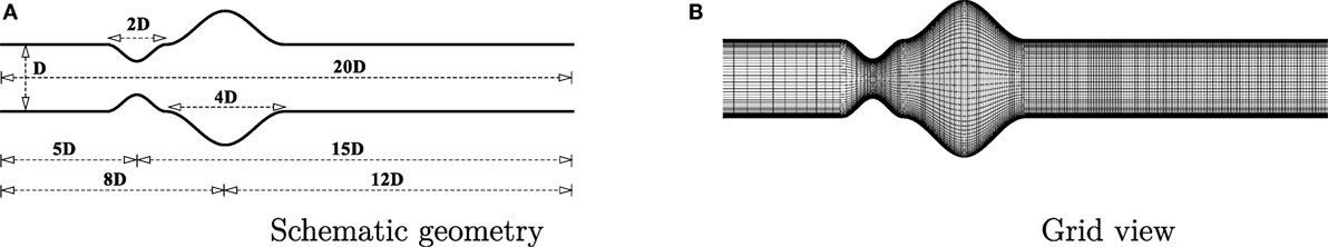
Figure 1. (A) The schematic geometry and (B) A portion of grid system (x − y view).

4. Physiological Flow

We obtained the physiological pulsatile velocity profile from the solution of a one-dimensional momentum equation where the pressure gradient is expressed as the Fourier series of time. This physiological velocity profile was first computed by Womersley (1955) for a tube by using the pressure gradient.

The steady part of the solution of the velocity field is obtained as:

$u\left(y\right)=\overline{U}\left[1-4\frac{y^2}{D^2}\right].$ (18)

The oscillatory part of the solution takes the following form:

$u\left(y\right)=\frac{A}{\mathit{in}\omega }\left[1-\frac{\text{cosh}\left(\sqrt{\frac{\rho }{\mu }\mathit{in}\omega }y\right)}{\text{cosh}\left(\sqrt{\frac{\rho }{\mu }\mathit{in}\omega }\frac{D}{2}\right)}\right].$ (19)

Using the definition of Womersley number, $\alpha =D\sqrt{\frac{\omega \rho }{\mu }}$, the full solution including the steady and oscillatory part for N harmonics can be written as:

$\begin{array}{ll}\hfill u\left(y,t\right)& =\overline{U}\left[1-4\frac{y^2}{D^2}\right]\\ & +{\displaystyle \sum _{n=1}^N}\frac{M_{n}A{h}^2}{\mathit{in}\mu {\alpha }^2}\left[1-\frac{\text{cosh}\left(\sqrt{\mathit{in}}\alpha \frac{y}{D}\right)}{\text{cosh}\left(\sqrt{\mathit{in}}\alpha \frac{1}{2}\right)}\right]e^{i\left(n\omega t+{\theta }_n\right)}.\end{array}$ (20)

The real part of this solution generates the physiological velocity profile at the inlet of the channel,

$\begin{array}{ll}\hfill u\left(y,t\right)& =\frac{A{D}^2}{n\mu {\alpha }^2{D}_r}[\text{cosh}{\theta }_1\text{cos}{\theta }_1\text{sinh}{\theta }_2\text{sin}{\theta }_2\text{cos}P\\ & -\text{sinh}{\theta }_1\text{sin}{\theta }_1\text{cosh}{\theta }_2\text{cos}{\theta }_2\text{cos}P\\ & -\text{cosh}{\theta }_1\text{cos}{\theta }_1\text{cosh}{\theta }_2\text{cos}{\theta }_2\text{sin}P\\ & -\text{sinh}{\theta }_1\text{sin}{\theta }_1\text{sinh}{\theta }_2\text{sin}{\theta }_2\text{sin}P+D_r\text{sin}P],\end{array}$ (21)

where,

${\varphi }_1=\alpha \sqrt{\frac{n}{2}}\frac{y}{D}$ (22)

${\varphi }_2=\frac{\alpha }{2}\sqrt{\frac{n}{2}}$ (23)

$P=n\omega t+{\theta }_n$ (24)

$D_r=\text{cos}{\text{h}}^2{\theta }_2{\text{cos}}^2{\theta }_2+\text{sin}{\text{h}}^2{\theta }_2{\text{sin}}^2{\theta }_2.$ (25)

In the above equations, A₀ and A are constants that correspond to the steady and oscillatory components of the pressure gradient; M_n, θ_n, and N resemble coefficients, phase angle, and the number of harmonics of the flow. Here, we are considering the first four harmonics of the pressure pulse; so, N = 4. $\omega \stackrel{\text{def}}{=}\frac{2\pi }{T}$, T and $i=\sqrt{-1}$ are the frequency of the pulsations, time period of a pulsating cycle and unit imaginary number, respectively. Where, bulk velocity, $\overline{U}$ depends on the Reynolds number. In the present study, for streamwise velocity, no slip condition has been used on the wall, but the normal velocity component changes as $v=\frac{\partial {\mathrm{\xi }}_2}{\mathrm{\partial }t}$. The zero gradient condition is applied at the outlet of the artery, where velocity gradient u and v are zero along the streamwise direction.

5. Non-Newtonian Viscosity Models

The shear rate varies over a range of 1–1200 s⁻¹ over a cardiac cycle in human arteries (Li et al., 2007). So, blood behaves as non-Newtonian fluid during some instants of the cardiac cycle. Hence, it is essential to study the non-Newtonian behavior of blood to understand the hemodynamics fully. Viscosity is constant against the shear rate in Newtonian fluids while it has an opposite behavior for the non-Newtonian fluids. There are four non-Newtonian viscosity models that are incorporated into the numerical simulation. The models are summarized in Table 1.

TABLE 1

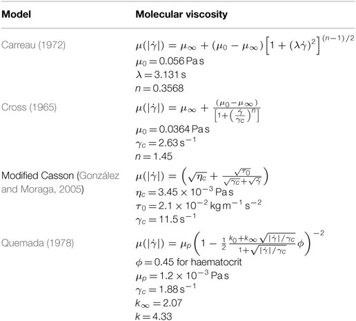
Table 1. Constitutive equations of non-Newtonian models.

6. Numerical Method

In this study, semi implicit pressure linked equation (SIMPLE) algorithm based on the finite-volume method has been used to solve the governing equations with collocated grid arrangements. To discretize the diffusion and convective terms in the momentum equations, a second-order accurate central difference has been used. The transient term was discretized using a three-point backward difference scheme with a constant time step Δt = 10⁻³. Since momentum equations are integrated over collocated grid arrangements, Rhie and Chow (1983) interpolation scheme is used to ensure strong pressure-velocity coupling. After discretization the velocity equations are solved by BI-CGSTAB of Van der Vorst (1992) solver and the Poisson type pressure correction equation is solved by incomplete Cholesky-conjugate (ICCGS) of Kershaw (1978) method. For the convergence of the velocity and pressure equations, the tolerance of the residuals is considered 10⁻⁷ and 10⁻⁸, respectively.

7. Code Validation

In the present study, the present numerical results are compared with the experimental results of Ahmed and Giddens (1983) considering the axisymmetric pipe with steady inlet velocity. The results are also compared with the numerical results of Damodaran et al. (1996) in the same Figure 2. Moreover, for this specific study, a grid independence test has also been performed as a part of code validation.

FIGURE 2

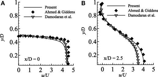
Figure 2. Comparison of streamwise velocity in two different axial locations (A) x/D = 0.0 and (B) x/D = 2.5 considering axisymmetric wall condition and compared with the experimental results of Ahmed and Giddens (1983) and numerical results of Damodaran et al. (1996) while Re = 500 and 75% stenosed model.

A grid resolution test is done to find the suitable grid arrangement where the numerical solution is independent of grid size. Different combinations of grid have been chosen here for this experimental purpose where: case 1: (x × y) = (240 × 90), Case 2: (x × y) = (300 × 80) and Case 3: (x × y) = (330 × 110). The Reynolds number has been fixed at 300 where the aneurysm is considered as 100% dilated and the stenosis as 60% constricted. Figure 3 illustrates the comparative results of Case 1, 2, and 3 in terms of the non-dimensionalized streamwise velocity. The velocity profiles plotted at the different axial locations and it is seen that results do not vary significantly while varying the grid arrangements. So, from these results it can be concluded that the results are not grid sensitive. Therefore, Case 3 (330 × 110) has been used in all other simulations for studying the non-Newtonian blood flow phenomena. The x − y view of a portion of the grid is shown here in Figure 1B and it shows that the grid distribution is remarkably refined near the upper and lower wall of the channel to accurately resolve the wall shear stress.

FIGURE 3

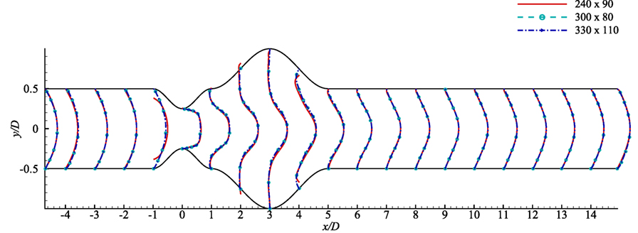
Figure 3. Grid resolution test with respect to streamwise velocity at various axial locations, i.e., x/D = inlet, x/D = −4.0, x/D = −3.0, x/D = −2.0, x/D = −1.0, x/D = 0.0, x/D = 1.0, x/D = 2.0, x/D = 3.0, x/D = 4.0, x/D = 5.0, …, x/D = 14 outlet based on three grid combinations, Case 1: solid line for 240 × 90 control volumes, Case 2: dashed line for 330 × 110 control volumes considering stenosis = 60% constricted and aneurysm = 100% dilated for Re = 300.

The geometry plays an important role in the arterial blood flow dynamics. Hence, disease as stenosis leading to a huge dilation causes severe deformation of the artery and thus remarkable flow diversion. As a consequence, wall pressure and wall shear stress along with streamlines experience a significant alteration in a diseased artery. In this section, we have presented the results of the numerical simulation of blood flow for both Newtonian and non-Newtonian cases through a diseased arterial model. The wall of the diseased model has been considered to be oscillating where the maximum amplitude of oscillation, A = 3 × 10⁻⁴.

8. Rheological Behavior in Terms of Wall Shear Stress and Wall Pressure

Wall shear stress (upper-wall) distribution across a 60% stenosed artery followed by 100% dilated arterial segment with Re = 300 is depicted in Figure 4A. The oscillating wall shear stress reaches the highest peak at the center of the stenosis and decreases inside the aneurysm in all viscosity models. However, the Carreau model experiences the highest magnitude while the Newtonian model always maintains the lowest wall shear stress throughout the artery.

FIGURE 4

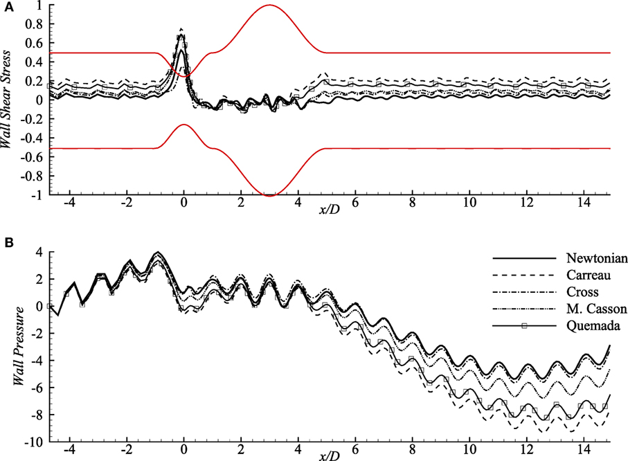
Figure 4. (A) Upper-wall pressure, p/ρU² and (B) upper-wall shear stress, τ_w/ρU² for different viscosity models while stenosis = 60% constricted and aneurysm = 100% dilated for Re = 300 where the amplitude of wall oscillation, A = 3 × 10⁻⁴.

Wall pressure (upper-wall) contributed by different rheological models, and also the Newtonian model is presented in Figure 4B that shows opposite patterns than that of the wall shear stress. The pulsatile flow creates significantly high pressure on the walls (upstream of the stent) in all models. It experiences a small drop in the constriction by all the rheological models where the Carreau model creates the local lowest and Cross, and Newtonian models cause higher wall pressure. The wall pressure decreases remarkably at the distant downstream location (near x/D = 12) of the aneurysm and maintains negative magnitudes after x/D = 4. Notably, the Newtonian and the Cross model cause the peak wall pressure near x/D = −1 while wall pressure decreases largely in Carreau model.

9. Laminar Flow Behavior

In the next paragraphs, we have particularly discussed the hemodynamic behavior regarding the parameters, i.e., streamlines, wall pressure, and wall shear stress for several Reynolds numbers and degrees of stenosis considering the Cross model that has already been mentioned in Section 5. However, the bulk velocity, $\overline{U}$ is computed here considering Re = 300 to study the laminar flow behavior.

9.1. Wall Pressure and Wall Shear Stress of Cross Model

Wall pressure (upper-wall) for various Reynolds numbers is compared in Figure 5A where the percentages of the stenosis and aneurysm are 60 and 100%, respectively. The wall pressure reaches its peak at the pre-stenosis zones and drops at the stenosis throat in all the fluids. The Re = 300 flow drops maximum and causes almost zero pressure at the stenosis center. The wall pressure increases again in the aneurysm but becomes negative at the distant downstream regions. However, the lower Reynolds numbers cause moderate wall pressure throughout the artery; neither tremendously high nor low.

FIGURE 5

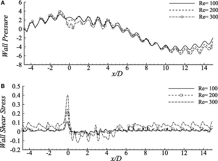
Figure 5. (A) Upper-wall pressure, p/ρU² and (B) upper-wall shear stress, τ_w/ρU² for different Reynolds numbers, i.e., Re = 100, 200, and 300 considering the Cross model when stenosis = 60% constricted and aneurysm = 100% dilated where the amplitude of wall oscillation, A = 3 × 10⁻⁴.

The aorta restricts the blood flow to cause a negative pressure on the arterial walls during the diastolic and systolic phases (Ku, 1997). It has been observed nearly zero pressure at the throat location and negative magnitudes at the distant downstream location of this diseased model which might restrict blood flow to different body parts (Young et al., 1975).

Figure 5B demonstrates the wall shear stress caused by various Reynolds numbers in the diseased artery for Cross model. The shear stress pattern seems to be very oscillating throughout the arterial segment for all the Reynolds number where the physiological profiles are also evident. Here, Re = 100 flow causes lower ranges of variation in the stress magnitudes, whereas the Re = 300 flow demonstrates highly chaotic pattern coupled with irregular sharp ends throughout the entire geometry. In fact, the peak stress that occurs at the stenosis throat, and the lowest peaks in the aneurysm, are caused by the flow with the highest Reynolds number. These characteristics match with the results by Tian et al. (2013).

Wall pressure and wall shear stress (upper wall) in the diseased artery for the Cross fluid has been depicted in Figure 6 considering different constriction percentages i.e., 40, 50, and 60% for Re = 300 in a 100% dilated artery. It is evident from the figure that increasing constriction causes more pressure drop at the stenosis center, but it remains unchanged for all the stenosis constrictions at the pre- and post-diseased segments which correspond to the results revealed by Young et al. (1975).

FIGURE 6

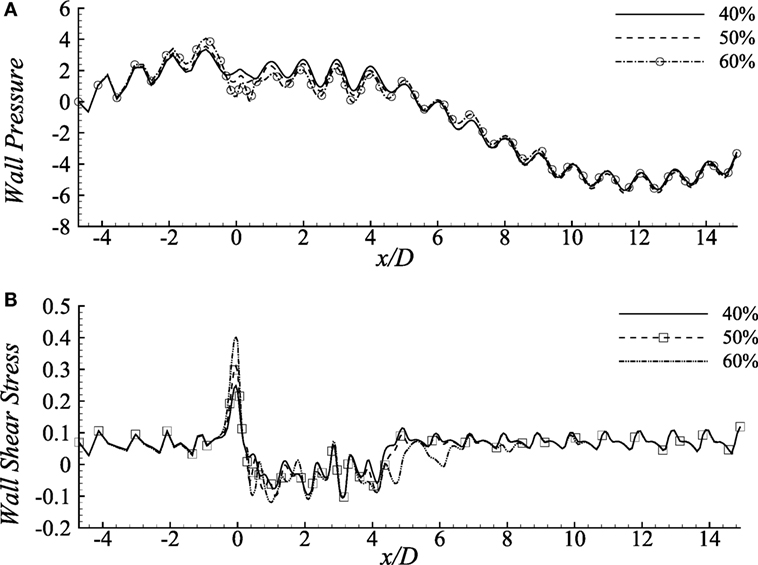
Figure 6. (A) Upper-wall pressure, p/ρU² and (B) Upper-wall shear stress, τ_w/ρU² for different stenosis percentages i.e., 40, 50, and 60% considering the Cross model when aneurysm = 100% dilated and Re = 300 where the amplitude of wall oscillation, A = 3 × 10⁻⁴.

The consequences of changing stenosis height on the wall shear stress are apparently visible in Figure 6B that is different from the previous results considering different Reynolds numbers. Wall shear stress increases at the stenosis throat, drops irregularly in the dilation and recovers at the post-aneurysm regions. However, both the positive and negative peaks are caused by the 40% constricted model. Again, shear stress becomes negative in the aneurysm for all the cases presented here.

9.2. Streamlines

Figure 7A illustrates the flow pattern in a 50% stenosed and 100% dilated arterial segment for Re = 100, 200, and 300. Figure 7Aa illustrates streamlines for Re = 100 where the fluid velocity is insignificant producing insignificant recirculation in the artery. Vortices are observed to form in the downstream of the stenosis and under the extended region of the vessel when the Reynolds number becomes 200. The velocity is very high at the stenosis throat in this case. However, the small vortices tend to become bigger in the aneurysm when the Reynolds number is 300. Moreover, two more pairs of small recirculation zones are observed in this case; one in the downstream of the stent and another in the upstream of the aneurysm. Hence, the curvatures of the geometry along with the oscillating wall condition might be responsible for this phenomenon.

FIGURE 7

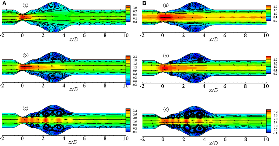
Figure 7. Streamlines while aneurysm = 100% dilated and Re = 300 for (A) various Reynolds numbers, i.e., (a) Re = 100, (b) Re = 200, and (c) Re = 300 and (B) various percentage of stenosis, i.e., (a) 40, (b) 50, and (c) 60% for Cross model where the amplitude of wall oscillation, A = 3 × 10⁻⁴.

Figure 7B represents the streamlines in a diseased artery for Re = 300 considering different stenosis percentages i.e., 40, 50, and 60%. It is evident from the Figures 7Ba,b that though the velocity range is same for the two cases, flow recirculation is significantly higher in the 50% stenosed model than the 40% one. However, the number of vortices increases as the percentage of stenosis is increased. Total five pairs of recirculation zones are observed at the post-lip regions causing huge flow recirculation in the arterial segment if the percentage is increased to 60%. Additionally, the effect of wall oscillation is apparently visible in all the diseased models.

The pulsatile condition of blood flow caused by the cyclic nature of blood contributes to forming flow recirculation. Considering this fact, recirculation regions in the diseased artery during different phases of a physiological cardiac cycle with 50% stenosis and 100% aneurysm for Re = 300 are illustrated in Figure 8. Several recirculation zones are found to form and gradually lose the velocity during the systolic phases through t/T = 0.0 − t/T = 3.0. However, large flow recirculation is observed in the aneurysm, but small eddies form at the post-stenotic zone at t/T = 3.0 that can be resembled as the late systolic phase. Flow velocity drops at early diastole in Figure 8E with small vortices and recovers the initial magnitude 1.4 through the late diastolic phases i.e., t/T = 7.0 − t/T = 10.0. In fact, the flow intensity of the late diastole matches with early systolic one.

FIGURE 8

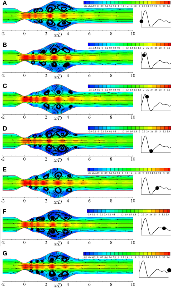
Figure 8. Streamlines at different physiological phases (A) t/T = 9.0, (B) t/T = 9.1, (C) t/T = 9.2, (D) t/T = 9.3, (E) t/T = 9.5, (F) t/T = 9.7, (G) t/T = 9.10 when aneurysm = 100% dilated and stenosis = 60% constricted for Re = 300 where the amplitude of wall oscillation, A = 3 × 10⁻⁴.

Figure 9 illustrates the flow recirculation scenario in laminar flow distribution in a diseased artery during different phases of a physiological cardiac cycle with 60% constricted stenosis and 100% dilated aneurysm. Total six pairs of vortices are observed to form at different streamwise locations of the arterial segment owing to the effect of Re = 500 where the moderately bigger pair forms in the dilation at t/T = 9.0. The vortices propagate toward the outlet throughout the cardiac cycle, and two moderately big pairs appear at the upstream and downstream of the aneurysm near the peak systole. After the peak systolic phase, vortices of the proximal region of the aneurysm becomes bigger than all other pairs. However, the vortex structures become exactly similar as the beginning phase during the end systolic phase that is shown in Figure 9D. The highest magnitude of velocity is also observed during this cardiac phase. Scenario for the diastolic phases are shown in Figures 9E–G, where the flow velocity decreases gradually and the bigger vortices propagate toward the downstream of the aneurysm.

FIGURE 9

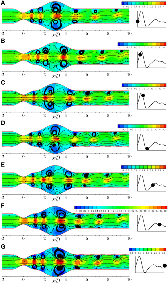
Figure 9. Streamlines at different physiological phases (A) t/T = 9.0, (B) t/T = 9.1, (C) t/T = 9.2, (D) t/T = 9.3, (E) t/T = 9.5, (F) t/T = 9.7, (G) t/T = 9.10 when aneurysm = 100% dilated and stenosis = 60% constricted for Re = 500 where the amplitude of wall oscillation, A = 3 × 10⁻⁴.

10. Laminar to Turbulent Transitional Flow Behavior

High Reynolds numbers are incorporated here to study the transitional behavior of the flow and Re = 750 has been used to compute the bulk velocity, $\overline{U}$.

10.1. Wall Shear Stress for Various Physiological Phases

We have studied the WSS (upper-wall) through a diseased arterial segment for Re = 300, Re = 500, and Re = 750 for different phases of a cardiac cycle. The results are depicted in Figure 10. These WSS diagrams are illustrated at different instants of the physiological pulsatile cycle.

FIGURE 10

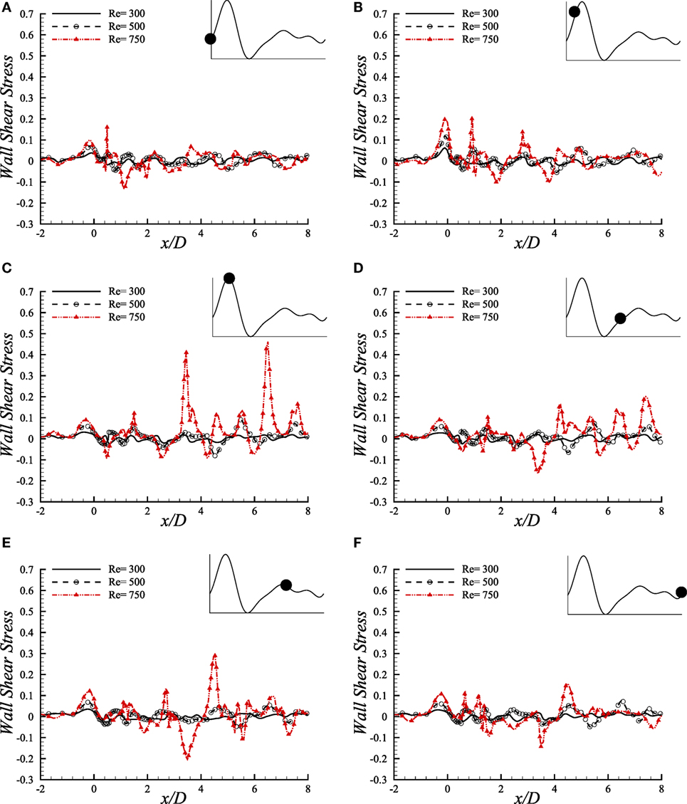
Figure 10. Upper-wall shear stress, τ_w/ρU², at different physiological phases (A) t/T = 9.0, (B) t/T = 9.1, (C) t/T = 9.2, (D) t/T = 9.5, (E) t/T = 9.7, (F) t/T = 9.10 when aneurysm = 100% dilated and stenosis = 60% constricted for various Reynolds numbers, i.e., Re = 300, Re = 500, and Re = 750 where the amplitude of wall oscillation, A = 3 × 10⁻⁴.

The magnitude of WSS for the three Reynolds numbers maintains a range of (−0.1, 0.2) in the beginning phase of a physiological cycle where the maximum Reynolds number causes the highest magnitude at the stenosis nose. As the flow experiences the systolic phases of a cardiac pulse, the range of WSS magnitude increases. At t/T = 9.1, the highest WSS is observed at the stenosis throat among all the phases where Re = 750 causes the highest value, and the Re = 300 flow causes the minimum one. However, the WSS pattern is chaotic at x/D = 1.0 where the flow experiences different phenomena owing to geometric effect.

During the peak systole, at t/T = 9.2, the instantaneous WSS magnitude of the Re = 750 flow shows irregular magnitudes in the post-stenosis region. It becomes high at the center of the aneurysm and also at the downstream region. All the Reynolds numbers contribute to a range of moderate WSS during the early diastolic phase, i.e., t/T = 9.5. Again, all the low ranged Reynolds number flows cause almost identical WSS patterns during the late diastolic phases and the end diastolic WSS matches with the early systolic one. Hence, during the entire cardiac pulse, it is evident that the Re = 300 and Re = 500 flow characteristics are more or less identical with variation in magnitudes throughout the arterial segment. But the Re = 750 flow becomes transitional to turbulent and shows different behavior in this study that may be difficult to predict the complete flow dynamics sometimes.

10.2. Wall Pressure for Various Physiological Phases

The comparative illustration of wall pressure (upper-wall) caused by different pulsatile phases of a cardiac cycle because of different Reynolds numbers is shown in Figure 11. Wall pressure decreases into negative magnitude and around zero in the stenosis for Re = 300 and Re = 500 and, but; Re = 750 flow causes the pressure to increase gradually after downstream of the stenosis and attain the highest at the aneurysm center during the beginning of the cardiac pulse. It drops to a range of negative magnitude at x/D = 3.0 during the next phase where all the Reynolds numbers cause almost identical wall pressure distribution.

FIGURE 11

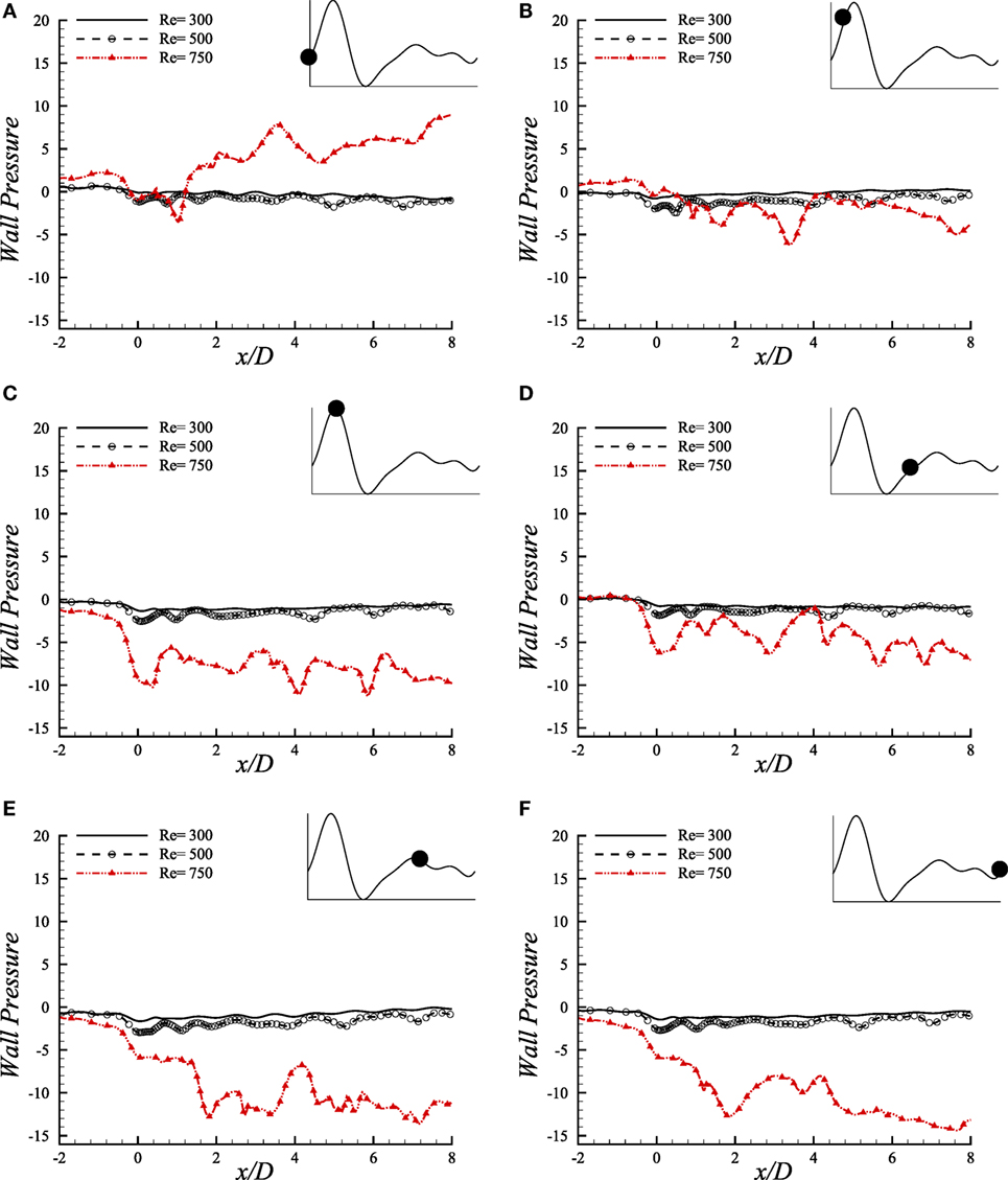
Figure 11. Upper-wall pressure, p/ρU², at different physiological phases (A) t/T = 9.0, (B) t/T = 9.1, (C) t/T = 9.2, (D) t/T = 9.5, (E) t/T = 9.7, (F) t/T = 9.10 when aneurysm = 100% dilated and stenosis = 60% constricted for various Reynolds numbers, i.e., Re = 300, Re = 500, and Re = 750 where the amplitude of wall oscillation, A = 3 × 10⁻⁴.

Interesting wall pressure distribution is observed at the peak systolic phase where all the flows cause the wall pressure to drop considerably at the center of the stenosis. It recovers to nearly zero magnitudes for the laminar flow conditions after this position while the high Reynolds number transitional to turbulent flow decreases the pressure more at about x/D = 4.0 and x/D = 6.0. However, all the flows experience a range of wall pressure between (−8, 0) during early diastole. The highest Reynolds number causes the flow to create highly negative wall pressure at the center of the stenosis during the peak diastole at t/T = 9.7. The laminar flows also drop at this location and then tries to recover the pressure to zero magnitudes, but Re = 750 flow creates irregular pressure distribution in the post-aneurysm regions during the peak and end of the diastolic phases.

10.3. Streamlines and Vorticity

Figure 12A illustrates the streamlines in the arterial segment for various Reynolds numbers using the Cross model. A range of velocity field (−0.2, 0.1) is observed to create negative flow field and thus recirculation in the near wall regions of the Re = 300 model that is shown in Figure 12Ai. However, the velocity maintains a high value near the central axis of the geometry and also symmetric vortex arrangement leaving the flow completely laminar.

FIGURE 12

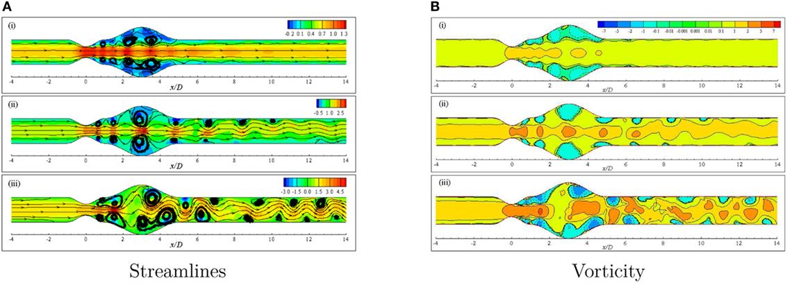
Figure 12. (A) Streamlines and (B) Vorticity when aneurysm = 100% dilated and stenosis = 60% constricted for various Reynolds numbers, i.e., (i) Re = 300, (ii) Re = 500, and (iii) Re = 750 visualizing the transition of the Cross model from laminar to translational where the amplitude of wall oscillation, A = 3 × 10⁻⁴.

The effect of increasing the Reynolds number to 500 is evident in Figure 12Aii. The streamlines become highly curved from the distal end of the stenosis up to the outlet position. Slight high velocity is observed around the central axis for a few streamwise locations, i.e., stenosis neck, the center of the bulge and proximal and distal ends of the aneurysm. A pair of large recirculation regions forms under cover of the dilation owing to the presence of negative velocity in these zones. Moreover, several eddy pairs are observed to form in the pre- and post-aneurysm regions that also resemble the effect of wall oscillation along with high Reynolds number.

A completely different phenomenon is noticed in streamlines for a diseased artery when the Reynolds number is 750. The flow becomes irregular with a wider range of velocity and extremely curved streamlines throughout the arterial segment. Numerous vortices are observed to form in different parts of the geometry that are asymmetric about the central axis. In fact, the flow loses its laminar characteristics at this Reynolds number and becomes translational to turbulent.

The vorticity that is given by $\omega =\frac{\mathrm{\partial }v}{\mathrm{\partial }x}-\frac{\mathrm{\partial }u}{\mathrm{\partial }y}$ describes the local spinning motion of the fluid. More insight of the circulatory phenomenon because of high constriction level coupled with high Reynolds number is depicted in Figure 12B. The vortex units rotate in the clockwise and anti-clockwise directions and give positive and negative values of ω, respectively. Clockwise rotations are represented by the solid lines while the dashed lines represent the anti-clockwise rotations.

Negative vortical structures are observed to form covering a large area (0.0 ≤ x/D ≤ 5.0) in the dilated portion of the artery in the Re = 300 model (Figure 12Bi). However, clockwise rotation of the flow is evident along the central axis of the artery with positive magnitude resembling laminar flow condition. The degree of flow separation increases as the Reynolds number increases. Multiple negative vortices form in the near wall regions throughout the entire arterial segment whereas, clockwise rotations are also observed along the central axis. Nevertheless, the flow scenario is different in the case of Re = 500 than the previous case due to highly dense positive and negative flow circulations.

Figure 12Biii shows the vorticity for the same geometry considering Re = 750 where translational to turbulent flow characteristics are apparently visible. The flow becomes irregular that does not follow any pattern. Highly negative rotations take place in different parts of the near wall regions following a complete asymmetric pattern about the central axis. The clockwise spinning also occurs in numerous separate zones. In essence, the flow phenomena change drastically when the Re = 750 that corresponds to transitional flow characteristics and the laminar to turbulent transition is assumed to occur when the Re > 500. Flow recirculation owing to the effect of different phases of a physiological pulsatile cycle for the transition to turbulent flow condition is depicted in Figure 13. Multiple vortices of various sizes are observed to form in different parts of the artery. Two moderate sized vortices form in the dilation; one under the upper wall and the other at the distal end of the aneurysm near the lower wall during t/T = 9.0. Number of recirculation regions and their length increase during the next cardiac cycle and the largest vortex form near about t/T = 9.1. After the peak systolic phase, the vortices get smaller and fewer during t/T = 9.2–9.5. The size of the vortices gets bigger, and the length of the recirculation region increases through the late diastolic phases. However, the asymmetric behavior of vortex generation and propagation is observed during the entire cardiac cycle due to the effect of laminar to turbulent flow transition.

FIGURE 13

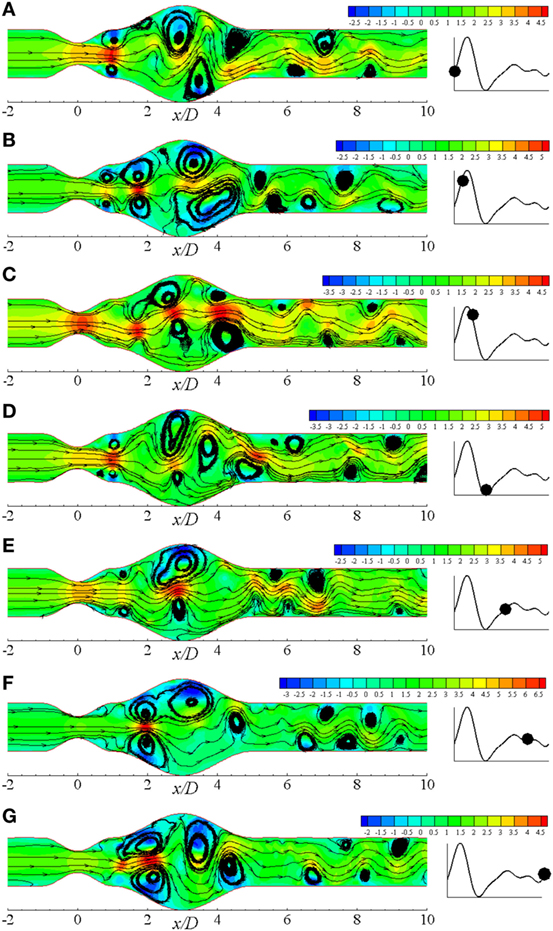
Figure 13. Streamlines in different physiological phases (A) t/T = 9.0, (B) t/T = 9.1, (C) t/T = 9.2, (D) t/T = 9.3, (E) t/T = 9.5, (F) t/T = 9.7, (G) t/T = 9.10 when aneurysm = 100% dilated and stenosis = 60% constricted for Re = 750 where the amplitude of wall oscillation, A = 3 × 10⁻⁴.

11. Conclusion

Hemodynamic factors, contributing to the deterioration of arterial diseases, have been numerically investigated in this paper. Finite-volume method has been used as the numerical technique, and the results have been presented in terms of hemodynamic parameters, i.e., wall pressure, wall shear stress, and streamlines for Re = 300, 500, and 750 considering sinusoidally oscillating wall condition for a coupled constricted and dilated channel. Comparisons are presented both for laminar and transitional flow considering various Reynolds numbers and also percentages of constriction keeping the aneurysm height fixed.

Both the Newtonian and non-Newtonian characteristics for wall pressure and wall shear stress are compared. The Newtonian model has presented comparatively lower wall shear stress and higher wall pressure in the arterial segment with 60% constricted stenosis than the other rheological models. Re = 300 causes a remarkable drop of wall pressure in the stenosis and at the distant downstream region. Moreover, it causes a very high shear stress at the stenosis throat with a severely oscillating pattern. The results for wall pressure are also compared varying the stenosis percentages with 100% dilated aneurysm. Wall pressure decreases maximum in the 60% stenosed model at the center of the stenosis, but it maintains an identical range at the downstream region. So, increasing Reynolds number affects the pressure distribution both at the center and downstream region while variation in stenosis percentage only affects the stenosis throat region. The effect of high wall shear stress of throat location prevails in the post-aneurysm downstream locations during the peak systolic phase as the flow experiences a laminar to turbulence transition. Moreover, the wall pressure falls tremendously during the entire diastole resulting serious health risk due to the effect of full occlusion.

The flow recirculation is found significant during the systolic phases for highly constricted stenosis and high Reynolds number in the Cross model. The flows become transitional to turbulent if the percentage of stenosis is increased more. Flow separation increases for the higher Reynolds number transitional flow in different parts of the geometry with a completely asymmetric pattern. Alongside, the streamlines also become chaotic and concentrated. High Reynolds number laminar flow contributes to the formation and propagation of multiple vortices in different parts of the artery in an axisymmetric manner whereas, chaotic and unpredictable recirculation occurs because of the laminar to turbulent flow transition.

Wall shear stress distribution plays a significant role in thrombus formation and progression which again contributes to causing stroke and even full occlusion (Bark and Ku, 2010). It can also cause endothelial or inner side damage of the arterial walls (Fry, 1968) which is apparently evident in our study at the stenosis throat. The resistance to flow, i.e., a significant drop of wall pressure becomes highly apparent at the downstream of the diseased artery and also at the throat which increases the risk to restrict the flow to different body parts (Young et al., 1975). Moreover, the highly stenosed and high Reynolds number model causes extremely remarkable flow recirculation inside the dilation along with high shear stress at the stenosis throat which is more likely to cause various vascular diseases.

Author Contributions

SS did the whole simulation and drafting of the manuscript. MMM supervised this project and edited the manuscript. MM worked as a co-supervisor and edited the manuscript.

Conflict of Interest Statement

The authors declare that the research was conducted in the absence of any commercial or financial relationships that could be construed as a potential conflict of interest.

Acknowledgments

SS acknowledges gratefully to North South University for providing financial support during this project. MMM would like to thank the PGI group for providing the University developer license of “PGI Accelerator Fortran/C/C++ compiler for a Workstation in Linux.”

Funding

This study was funded by North South University.

References

Ahmed, S. A., and Giddens, D. P. (1983). Velocity measurements in steady flow through axisymmetric stenoses at moderate reynolds numbers. J. Biomech. 16, 505–516. doi: 10.1016/0021-9290(83)90096-9

PubMed Abstract | CrossRef Full Text | Google Scholar

Bark, D. L. Jr., and Ku, D. N. (2010). Wall shear over high degree stenoses pertinent to atherothrombosis. J. Biomech. 43, 2970–2977. doi:10.1016/j.jbiomech.2010.07.011

PubMed Abstract | CrossRef Full Text | Google Scholar

Berg, P., Stucht, D., Janiga, G., Beuing, O., Speck, O., and Thévenin, D. (2014). Cerebral blood flow in a healthy circle of willis and two intracranial aneurysms: computational fluid dynamics versus four-dimensional phase-contrast magnetic resonance imaging. J. Biomech. Eng. 136, 041003. doi:10.1115/1.4026108

PubMed Abstract | CrossRef Full Text | Google Scholar

Berger, S. A., and Jou, L. D. (2000). Flows in stenotic vessels. Annu. Rev. Fluid Mech. 32, 347–382. doi:10.1146/annurev.fluid.32.1.347

CrossRef Full Text | Google Scholar

Carreau, P. J. (1972). Rheological equations from molecular network theories. Trans. Soc. Rheol. 16, 99–127. doi:10.1122/1.549276

CrossRef Full Text | Google Scholar

Cross, M. M. (1965). Rheology of non-newtonian fluids: a new flow equation for pseudoplastic systems. J. Colloid Sci. 20, 417–437. doi:10.1016/0095-8522(65)90022-X

CrossRef Full Text | Google Scholar

Damodaran, V., Rankin, G. W., and Zhang, C. (1996). Numerical study of steady laminar flow through tubes with multiple constrictions using curvilinear co-oordinates. Int. J. Numer. Methods Fluids 23, 1021–1041. doi:10.1002/(SICI)1097-0363(19961130)23:10<1021::AID-FLD449>3.0.CO;2-D

CrossRef Full Text | Google Scholar

Deplano, V., Knapp, Y., Bertrand, E., and Gaillard, E. (2007). Flow behaviour in an asymmetric compliant experimental model for abdominal aortic aneurysm. J. Biomech. 40, 2406–2413. doi:10.1016/j.jbiomech.2006.11.017

CrossRef Full Text | Google Scholar

Egelhoff, C. J., Budwig, R. S., Elger, D. F., Khraishi, T. A., and Johansen, K. H. (1999). Model studies of the flow in abdominal aortic aneurysms during resting and exercise conditions. J. Biomech. 32, 1319–1329. doi:10.1016/S0021-9290(99)00134-7

PubMed Abstract | CrossRef Full Text | Google Scholar

Ellahi, R., Rahman, S. U., Gulzar, M. M., Nadeem, S., and Vafai, K. (2014). A mathematical study of non-newtonian micropolar fluid in arterial blood flow through composite stenosis. Appl. Math. Inf. Sci. 8, 1567–1573. doi:10.12785/amis/080410

CrossRef Full Text | Google Scholar

Fry, D. L. (1968). Acute vascular endothelial changes associated with increased blood velocity gradients. Circ. Res. 22, 165–197. doi:10.1161/01.RES.22.2.165

CrossRef Full Text | Google Scholar

George, S. J., and Johnson, J. (2010). Atherosclerosis: Molecular and Cellular Mechanisms. Weinheim: John Wiley & Sons.

Google Scholar

González, H. A., and Moraga, N. O. (2005). On predicting unsteady non-newtonian blood flow. Appl. Math. Comput. 170, 909–923. doi:10.1016/j.amc.2004.12.029

CrossRef Full Text | Google Scholar

Harloff, A., Zech, T., Wegent, F., Strecker, C., Weiller, C., and Markl, M. (2013). Comparison of blood flow velocity quantification by 4D flow MR imaging with ultrasound at the carotid bifurcation. Am. J. Neuroradiol. 34, 1407–1413. doi:10.3174/ajnr.A3419

PubMed Abstract | CrossRef Full Text | Google Scholar

Karimi, S., Dadvar, M., Dabagh, M., Jalali, P., Modarress, H., and Dabir, B. (2013). Simulation of pulsatile blood flow through stenotic artery considering different blood rheologies: comparison of 3D and 2D-axisymmetric models. Biomed. Eng. Appl. Basis Commun. 25, 1350023. doi:10.4015/S1016237213500233

CrossRef Full Text | Google Scholar

Kershaw, D. S. (1978). The incomplete cholesky–conjugate gradient method for the iterative solution of systems of linear equations. J. Comput. Phys. 26, 43–65. doi:10.1016/0021-9991(78)90098-0

CrossRef Full Text | Google Scholar

Ku, D. N. (1997). Blood flow in arteries. Annu. Rev. Fluid Mech. 29, 399–434. doi:10.1146/annurev.fluid.29.1.399

CrossRef Full Text | Google Scholar

Kumar, B. V. R., and Naidu, K. B. (1996). Hemodynamics in aneurysm. Comput. Biomed. Res. 29, 119–139. doi:10.1006/cbmr.1996.0011

CrossRef Full Text | Google Scholar

Li, M. X., Beech-Brandt, J. J., John, L. R., Hoskins, P. R., and Easson, W. J. (2007). Numerical analysis of pulsatile blood flow and vessel wall mechanics in different degrees of stenoses. J. Biomech. 40, 3715–3724. doi:10.1016/j.jbiomech.2007.06.023

PubMed Abstract | CrossRef Full Text | Google Scholar

Long, Q., Xu, X. Y., Ramnarine, K. V., and Hoskins, P. (2001). Numerical investigation of physiologically realistic pulsatile flow through arterial stenosis. J. Biomech. 34, 1229–1242. doi:10.1016/S0021-9290(01)00100-2

PubMed Abstract | CrossRef Full Text | Google Scholar

Moayeri, M. S., and Zendehbudi, G. R. (2003). Effects of elastic property of the wall on flow characteristics through arterial stenoses. J. Biomech. 36, 525–535. doi:10.1016/S0021-9290(02)00421-9

PubMed Abstract | CrossRef Full Text | Google Scholar

Otani, T., Nakamura, M., Fujinaka, T., Hirata, M., Kuroda, J., Shibano, K., et al. (2013). Computational fluid dynamics of blood flow in coil-embolized aneurysms: effect of packing density on flow stagnation in an idealized geometry. Med. Biol. Eng. Comput. 51, 901–910. doi:10.1007/s11517-013-1062-5

PubMed Abstract | CrossRef Full Text | Google Scholar

Paramasivam, V., Muthusamy, K., and Kadir, M. R. A. (2010). “Application of computational fluid dynamics in assessing the hemodynamics in abdominal aortic aneurysms,” in Biomedical Engineering and Sciences: 2010 IEEE EMBS Conference (Kualalumpur: IEEE), 32–37.

Google Scholar

Pedley, T. J. (1994). High reynolds number flow in tubes of complex geometry with application to wall shear stress in arteries. Symp. Soc. Exp. Biol. 49, 219–241.

PubMed Abstract | Google Scholar

Perktold, K. (1986). On the paths of fluid particles in an axisymmetrical aneurysm. J. Biomech. 20, 311–317. doi:10.1016/0021-9290(87)90297-1

CrossRef Full Text | Google Scholar

Quemada, D. (1978). Rheology of concentrated disperse systems III. General features of the proposed non-newtonian model. comparison with experimental data. Rheol. Acta 17, 643–653. doi:10.1007/BF01522037

CrossRef Full Text | Google Scholar

Rabby, M. G., Sultana, R., Shupti, S. P., and Molla, M. M. (2014). Laminar blood flow through a model of arterial stenosis with oscillating wall. Int. J. Fluid Mech. Res. 41, 417–429. doi:10.1615/InterJFluidMechRes.v41.i5.30

CrossRef Full Text | Google Scholar

Razavi, A., Shirani, E., and Sadeghi, M. R. (2011). Numerical simulation of blood pulsatile flow in a stenosed carotid artery using different rheological models. J. Biomech. 44, 2021–2030. doi:10.1016/j.jbiomech.2011.04.023

CrossRef Full Text | Google Scholar

Rhie, C., and Chow, W. L. (1983). Numerical study of the turbulent flow past an airfoil with trailing edge separation. AIAA J. 21, 1525–1532. doi:10.2514/3.8284

CrossRef Full Text | Google Scholar

Saleem, N., Hayat, T., and Alsaedi, A. (2014). A hydromagnetic mathematical model for blood flow of carreau fluid. Int. J. Biomath. 7, 1450010. doi:10.1142/S1793524514500107

CrossRef Full Text | Google Scholar

Shupti, S. P., Rabby, M. G., and Molla, M. M. (2015). Rheological behavior of physiological pulsatile flow through a model arterial stenosis with moving wall. J. Fluids 22, 546716. doi:10.1155/2015/546716

CrossRef Full Text | Google Scholar

Shupti, S. P., Sultana, R., Rabby, M. G., and Molla, M. M. (2013). Pulsatile laminar flows in a dilated channel using Cartesian curvilinear coordinates. Univ. J. Mech. Eng. 1, 98–107. doi:10.13189/ujme.2013.010304

CrossRef Full Text | Google Scholar

Su, B., Huo, Y., Kassab, G. S., Kabinejadian, F., Kim, S., Liang Leo, H., et al. (2014). Numerical investigation of blood flow in three-dimensional porcine left anterior descending artery with various stenoses. Comput. Biol. Med. 47, 130–138. doi:10.1016/j.compbiomed.2014.01.001

PubMed Abstract | CrossRef Full Text | Google Scholar

Thomson, J. F., Thames, F., and Mastin, C. (1974). Automatic numerical generation of body-fitted curvilinear coordinate system for field containing any number of arbitrary two dimentional bodies. J. Comput. Phys. 15, 299–319. doi:10.1016/0021-9991(74)90114-4

CrossRef Full Text | Google Scholar

Tian, F., Zhu, L., Fok, P., and Lu, X. (2013). Simulation of a pulsatile non-Newtonian flow past a stenosed 2D artery with atherosclerosis. Comput. Biol. Med. 43, 1098–1113. doi:10.1016/j.compbiomed.2013.05.023

PubMed Abstract | CrossRef Full Text | Google Scholar

Tu, C., and Deville, M. (1996). Pulsatile flow of non-newtonian fluids through arterial stenoses. J. Biomech. 29, 899–908. doi:10.1016/0021-9290(95)00151-4

PubMed Abstract | CrossRef Full Text | Google Scholar

Tu, C., Deville, M., Dheur, L., and Vanderschuren, L. (1992). Finite element simulation of pulsatile flow through arterial stenosis. J. Biomech. 25, 1141–1152. doi:10.1016/0021-9290(92)90070-H

PubMed Abstract | CrossRef Full Text | Google Scholar

Upadhyay, V., Chaturvedi, S. K., and Upadhyay, A. (2012). A mathematical model on effect of stenosis in two phase blood flow in arteries remote from the heart. J. Int. Acad. Phys. Sci. 16, 247–257.

Google Scholar

Van der Vorst, H. A. (1992). Bi-cgstab: a fast and smoothly converging variant of bi-cg for the solution of nonsymmetric linear systems. SIAM J. Sci. Statis. Comput. 13, 631–644. doi:10.1137/0913035

CrossRef Full Text | Google Scholar

Volokh, K. Y., and Vorp, D. A. (2008). A model of growth and rupture of abdominal aortic aneurysm. J. Biomech. 41, 1015–1021. doi:10.1016/j.jbiomech.2007.12.014

PubMed Abstract | CrossRef Full Text | Google Scholar

Womersley, J. R. (1955). Method for the calculation of velocity, rate of flow and viscous drag in arteries when the pressure gradient is known. J. Physiol. 127, 553–563. doi:10.1113/jphysiol.1955.sp005276

CrossRef Full Text | Google Scholar

Yip, T. H., and Yu, S. C. M. (2001). Cyclic transition to turbulence in rigid abdominal aortic aneurysm models. Fluid Dyn. Res. 29, 81–113. doi:10.1016/S0169-5983(01)00018-1

CrossRef Full Text | Google Scholar

Young, D. F., Cholvin, N. R., and Roth, A. C. (1975). Pressure drop across artificially induced stenoses in the femoral arteries of dogs. Circ. Res. 36, 735–743. doi:10.1161/01.RES.36.6.735

PubMed Abstract | CrossRef Full Text | Google Scholar

Zendehbudi, G. R., and Moayeri, M. S. (1999). Comparison of physiological and simple pulsatile flows through stenosed arteries. J. Biomech. 32, 959–965. doi:10.1016/S0021-9290(99)00053-6

PubMed Abstract | CrossRef Full Text | Google Scholar

Zhang, X., Li, X., Xu, B., and Wang, F. (2009). “Numerical simulation of blood flow in internal carotid artery aneurysm,” in Biomedical Engineering and Informatics, 2009: 2nd International Conference (Tianjin: IEEE), 1–4.

Google Scholar