Modeling Temperature Variations in MILD Combustion Using MuSt-FGM

1. Introduction

Moderate or intense low oxygen dilution (MILD) combustion is a relatively new technology that provides low emissions and high efficiency. The basic idea in MILD combustion is to recirculate the burned flue gases back, mix them with the reactants so that the combustion occurs at a milder rate (as the acronym suggests), and the temperature increase is much lower than in a conventional flame. It provides high efficiency, and reduces the emissions of CO, SO_x, soot, and especially NO_x (Cavaliere and de Joannon, 2004; Derudi and Rota, 2011; De Joannon et al., 2012), owing to lower flame temperatures. There are different definitions of MILD combustion in the literature. Cavaliere and de Joannon (2004) define MILD combustion as the combustion mode where the temperature of the reactants are high enough to autoignite, and the temperature increase in the combustor is less than the autoignition temperature in Kelvin. Wünning and Wünning (1997) make the distinction based on the furnace temperature and exhaust recirculation rate. More recently, Evans et al. (2017) came up with a new definition based on the unique S-curve of MILD combustion: there are no jumps between ignition and extinction events but a continuous ignition curve. They analyzed different premixed and non-premixed MILD cases and have shown that their definition agreed well with the experimental observations of gradual ignition in MILD conditions. Even though there are some discussions on which definition suits MILD combustion the best, overall characteristics are nevertheless well agreed on.

The beneficial characteristics of MILD combustion attracted attention from the combustion research and development communities. It has been applied to the steel and metallurgy industries starting from the 1990s (Li et al., 2011). More recently, opportunities of applying MILD combustion to gas turbines (Duwig et al., 2007; Albin et al., 2015; Kruse et al., 2015; Perpignan et al., 2018) and gasification processes (Tang et al., 2010) have been investigated. However, potential of MILD combustion is beyond these applications, as mentioned in Li et al. (2011). Therefore, additional efforts need to be made to fully understand the physical mechanisms in MILD combustion, and thereby expand its application areas and fulfill its potential.

To explore the physical mechanisms of MILD combustion, numerous experimental studies have been performed, with lab scale burners of different complexities. One of the most used configurations is the jet in hot coflow (JHC) configuration, where a hot and diluted oxidizer is created using a secondary burner, and a fuel jet is issued into this diluted oxidizer. Fuel and oxidizer mix via diffusion and entrainment, and the flame is stabilized by autoignition at a certain distance from the fuel nozzle. This way, the diluted nature of MILD combustion is imitated, without the need for real exhaust gas recirculation. The JHC configuration was utilized in both laminar (Sepman et al., 2013a,b) and turbulent conditions (Dally et al., 2002; Oldenhof et al., 2011; Duwig et al., 2012; Ma and Roekaerts, 2016) to achieve MILD combustion.

MILD combustion has been studied extensively using computational fluid dynamics (CFD) as well. Abtahizadeh et al. and Sepman et al. investigated the laminar JHC burner from University of Groningen using detailed chemistry (Abtahizadeh et al., 2013; Sepman et al., 2013b). In the former study, the effects of preheating and dilution were investigated, and it was found that in the presence of both preheating and dilution, the flame transitions into the MILD regime, and stabilizes via autoignition. In the latter study, it was demonstrated that the MILD case emits much less NO compared to the conventional flame. A reasonable agreement between experimental and numerical results was obtained in both cases. De et al. (2011) employed the eddy dissipation concept (EDC) with a Reynolds averaged Navier-Stokes (RANS) model to simulate the JHC experiments from Delft University of Technology (Oldenhof et al., 2011). They predicted the radial profiles of temperature and velocity reasonably well, but failed to match the lift-off heights found in the experiments. Another RANS study to investigate the JHC burner from The University of Adelaide was conducted by Christo and Dally (2005). They employed different turbulence and chemistry models, and concluded that the EDC with the standard k-ϵ turbulence model produces the best agreement with the experimental results. In addition, they stressed that preferential diffusion effects should be taken into account due to the high hydrogen content in the fuel. There have been several large eddy simulations (LES) of JHC burners as well. Kulkarni and Polifke applied a flamelet/progress variable (FPV) approach and found that the heat losses in the coflow are crucial in determining the lift-off height (Kulkarni and Polifke, 2013). Ihme et al. (2012) employed an FPV formulation with a three stream approach to account for the outermost cold air stream in the experiments from Adelaide. They also tried to fit the controlling variables to accurately represent the species profile of the coflow. In their computations, addition of the third stream yielded satisfactory results in terms of temperature and species profiles. In all the turbulent JHC simulations; turbulence, chemistry, and their interactions were modeled simultaneously. Therefore, it is difficult to judge which part of the modeling effort is failing when the results are not matching well with the experiments.

In order to understand the complex physical and chemical phenomena and their interactions in MILD combustion, detailed calculations need to be performed before any modeling effort. Minamoto et al. carried out the first 3D DNSs of MILD combustion (Minamoto et al., 2013, 2014). They simulated a premixed MILD system whose composition is obtained via 1D laminar flames, and compared the results with a conventional premixed case to examine differences in flame structures. They concluded that there are strong chemically reacting zones in the MILD regime, but unlike traditional premixed flames, the reaction layers are not sheet like and they interact with each other. Although their studies shed light on MILD combustion flame structures for premixed cases, they do not provide any interpretation for spontaneous mixing and chemistry, which is the case in many MILD systems including JHC experiments. van Oijen (2013) performed 2D DNS of autoigniting mixing layers representative of the JHC burner in Dally et al. (2002) and compared the results with 1D diffusive layer simulation results. His results show that the ignition delay times for the diffusive layer simulations and the 2D DNS are almost the same, and they are strongly dependent on preferential diffusion effects. Nevertheless, real turbulence effects could not be reproduced in his study since 2D turbulence lacks vortex stretching phenomena and has an inverse energy cascade. In addition, heat loss and the resulting non-uniform temperature profile of the coflow found in the experiments were not taken into account. In their 3D DNS study, Göktolga et al. (2015) demonstrated that the heat loss effects have a large influence on the ignition delay, and even in 3D turbulence the effects of preferential diffusion are still of utmost importance. Furthermore, they showed that due to flame curvature-preferential diffusion interactions, the species scatter differently in the composition space. More recently, Doan et al. (2018) investigated a MILD combustion case with 3D DNS, including mixture fraction and chemical progress variations in the inflow boundary conditions. They found out that ignition front, premixed flames, and non-premixed flames all coexist, without the presence of triple flame structures. Swaminathan (2019) has recently compiled the DNS works on MILD combustion. He concludes that the reactions zones in MILD combustion display autoignition characteristics of both non-premixed and premixed flames. He further deduces that reaction regions can be seen as homogeneous reactors and thus can be modeled accurately with tabulated chemistry using perfectly stirred reactors as canonical flames.

In combustion modeling, it is often the case that the total enthalpy at each mixture fraction does not deviate from the value corresponding to adiabatic mixing. For many cases this is a valid assumption (Cabra et al., 2002; Barlow et al., 2005). However, if there is heat loss through the combustor walls (Lammel et al., 2012), or the flame is considerably radiating (Dally et al., 1998), or there are heat losses even before the mixture enters the combustor (Dally et al., 2002; Mendez et al., 2015); then this assumption is no longer valid and the effects of the enthalpy change need to be modeled. In the context of flamelet based chemistry tabulation methods such as flamelet/progress variable (FPV) (Pierce and Moin, 2004), flame prolongation of ILDM (FPI) (Gicquel et al., 2000), and FGM; the most often used approach is to utilize the enthalpy as an additional control variable (Fiorina et al., 2003; Ihme and Pitsch, 2008; Donini et al., 2013).

In this study, the conditions to simulate are selected as the HM1 case of the Adelaide JHC case (Dally et al., 2002), because it is shown to operate in MILD combustion. In those experiments, there is a large variation in the oxidizer temperature when the oxidizer enters the primary combustor, because of the cooling jacket around the fuel (Dally et al., 2002). In some studies, this effect was completely ignored (Afarin and Tabejamaat, 2013; Chen et al., 2017). However, it was shown in Göktolga et al. (2015) that this temperature variation is of utmost importance for the ignition delay and related chemistry. Therefore, to have an accurate description of this case, taking the species and especially temperature variations in the oxidizer into account is a must, as has been addressed by several studies before (Ihme and See, 2011; Ihme et al., 2012; Sarras et al., 2014; Ma and Roekaerts, 2016). Ihme and See (2011) have utilized a three stream FPV approach to include the effects of the air shroud present in the Adelaide JHC experiments. They have introduced an extra control variable called oxidizer split, which was set to 0 and 1 for the diluted coflow and air shroud regions, respectively. By varying the progress variable and the oxidizer split in the coflow region, they included the temperature and species variations in the coflow. They applied this approach to simulate the HM3 (Y_O2 = 9%) case of the Adelaide JHC case, and later their work was extended by Ihme et al. (2012) to model the HM1 and HM2 (Y_O2 = 3% and Y_O2 = 6%, respectively) cases as well. Sarras et al. (2014) also introduced an extra mixture fraction to take the oxygen variations in the coflow, and further utilized enthalpy deficit to model the temperature variation, to model the Delft JHC burner (Oldenhof et al., 2011). Ma and Roekaerts (2016) used enthalpy directly as a control variable to model the enthalpy deficit due to intense droplet evaporation, to simulate spray combustion operating under MILD conditions.

With ever growing chemical reaction mechanisms, the use of detailed chemistry in 3D computations become more prohibitive despite the advances in computational hardware. Not only are there many species for which the transport equations are solved, but also the time step needed are quite small because of the stiffness of the chemical reactions. There are many chemistry reduction models proposed to decrease the computational requirements. One of them is flamelet generated manifolds (FGM) (van Oijen and de Goey, 2000). In FGM, it is assumed that a 3D flame is composed of 1D flamelets (Peters, 1984); and the composition space can be represented with lower dimensional manifold. To model a flame with FGM; 1D flames are solved, necessary thermo-chemical variables are stored in FGM tables as functions of a few control variables, and then transport equations for only those control variables are solved and required thermo-chemical are retrieved from the FGM tables. Göktolga et al. showed that for MILD combustion, standard FGM cannot model both the pre-ignition and oxidation regions accurately, and proposed a multistage (MuSt) FGM (Göktolga et al., 2017). In this method, different progress variables are used for each combustion stage to capture those stages properly. Because in FGM the diffusion processes are modeled as well, effects like flame propagation can be captured adequately. In Göktolga et al. (2017), it was shown that another very crucial flame stabilization mechanism in MILD combustion, namely the autoignition, can be captured with MuSt-FGM.

The aim of this study to model the effects of temperature variation in the oxidizer of the Adelaide JHC case using MuSt-FGM. In the remaining following sections the numerical methods and simulation setup are detailed, results are presented, and some conclusions are drawn.

2. Numerical Methods and Simulation Setup

As mentioned earlier, in an FGM study, firstly 1D flamelet calculations are performed. In this study, counter-flow flames with a strain rate of 200 s⁻¹ are used as the flamelet type. The details of the counter-flow canonical configuration can be found in Vasavan et al. (2018). The calculations are performed using the 1D flame code called Chem1D (Somers, 1994). As the control variable representing the mixing between the fuel and the oxidizer, transported mixture fraction Z_t is used. Since this is a MuSt-FGM study, the chemical progress for the pre-ignition and oxidation stage are represented by two different progress variables. In this study they are selected as ${{Y}}_1=Y_{H{O}_2}$ and ${{Y}}_2=Y_{H_{2}O}$, because the fuel in this case contains 50% hydrogen by volume, and thus the reactions are dominated by hydrogen chemistry. Two different tables for the pre-ignition and oxidation region are created with ${{Y}}_1=Y_{H{O}_2}$ and ${{Y}}_2=Y_{H_{2}O}$, transport equations for both ${{Y}}_1$ and ${{Y}}_2$ are solved simultaneously, and the table lookup is performed depending on which stage the combustion is. Further details of the MuSt-FGM method can be found in Göktolga et al. (2017).

In the DNS calculations, in house developed code (Bastiaans et al., 2001; Groot, 2003; Van Oijen et al., 2007) was used. In the code, fully compressible Navier-Stokes equations are solved together with the transport equations for control variables, which read:

$\begin{array}{ll}\frac{\partial \rho }{\partial t}+\frac{\partial (\rho u_i)}{\partial x_i}=0& (1)\end{array}$

$\begin{array}{ll}\rho \frac{\partial u_j}{\partial t}+\rho u_i\frac{\partial u_j}{\partial x_i}=-\frac{\partial p}{\partial x_j}+\frac{\partial {\sigma }_{ij}}{\partial x_i}& (2)\end{array}$

$\begin{array}{ll}\rho \frac{\partial Z_t}{\partial t}+\rho u_i\frac{\partial Z_t}{\partial x_i}=\frac{\partial }{\partial x_i}\left(\frac{\lambda }{c_p}\frac{\partial Z_t}{\partial x_i}\right),& (3)\end{array}$

$\begin{array}{ll}\rho \frac{\partial {Y}}{\partial t}+\rho u_i\frac{\partial {Y}}{\partial x_i}=\frac{\partial }{\partial x_i}\left(\frac{\lambda }{L{e}_{{Y}}{c}_p}\frac{\partial {Y}}{\partial x_i}\right)+{\omega }_{{Y}},& (4)\end{array}$

$\begin{array}{ll}\rho c_v\frac{\partial T}{\partial t}+\rho c_v{u}_i\frac{\partial T}{\partial x_i}=\frac{\partial }{\partial x_i}\left(\lambda \frac{\partial T}{\partial x_i}\right)-p\frac{\partial u_i}{\partial x_i}+{\sigma }_{ij}\frac{\partial u_i}{\partial x_j}+q& (5)\end{array}$

where the variables solved for are density ρ, velocity u_j, transported mixture fraction Z_t, progress variable ${Y}$, and temperature T. c_v and c_p are specific heats at constant volume and pressure, λ is thermal conductivity, σ is the stress tensor, $L{e}_{{Y}}$ and ${\omega }_{{Y}}$ are Lewis number and chemical source term of the progress variable, q is the heat release rate in W/m³. Variables like c_v, q, λ, as well as the viscosity used in stress term calculation are looked up from the MuSt-FGM tables. For numerical discretization, an implicit 6th order compact finite difference (FD) scheme (Lele, 1992) for diffusive terms, and a 5th order FD scheme with upwinding (de Lange, 2007) for the convective terms are employed. The tri-diagonal system originating from the implicit derivatives is solved using the Thomas algorithm. A 3rd order explicit Runge-Kutta scheme is utilized to perform the time integration. To avoid numerical instabilities at the boundaries, Navier-Stokes characteristic boundary conditions (NSCBC) (Poinsot and Lelef, 1992) are implemented.

As mentioned, in this study the JHC experiments from the University of Dally et al. (2002) are used as the baseline. The reason for selecting this case was that it mimics MILD combustion conditions properly and has extensive experimental data. From the three compositions studied in Dally et al. (2002), the HM1 case was selected because it contains the least amount of oxygen and thus represents MILD conditions the best.

In an industrial combustor, MILD conditions are often obtained via internal recirculation of flue gases. In the Adelaide JHC experimental setup, to mimic those conditions, a diluted oxidizer stream is created using a secondary burner and mixing hot combustion products from this secondary burner with fresh air at varying levels to control the oxygen levels. A cold fuel jet is issued into the diluted hot oxidizer, the two streams mix, and MILD combustion occurs in the primary burner. There is also a cold air tunnel around the hot oxidizer stream, which does not affect the combustion in the primary burner until 100 mm downstream from the fuel jet exit. This air stream is ignored in this study.

Experimentally intended constant temperature and species boundary conditions for the HM1 case are given in Table 1. However, due to experimental imperfections, in reality these variables are not constant in space and deviate from the intended conditions. Especially the temperature profile of the diluted oxidizer shows large variations due to the effect of cooling around the fuel pipe. Radial profiles of species and temperature were measured in the experiments at different axial locations. The measurements at z = 4 mm are assumed as the actual boundary conditions. In this work, simulations with only the real experimental conditions are performed, and they are referred to as “actual” profile cases. Profiles of temperature and oxidizer for the actual profile case as applied in the simulations are shown in Figure 1.

TABLE 1

Table 1. Intended boundary conditions for the HM1 case of the JHC experiments.

FIGURE 1

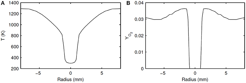
Figure 1. Inlet radial profiles of temperature (A) and Y_O2 (B), scaled from the measured experimental values.

DNS computations were performed in the form of igniting mixing layers. A schematic of the computational domain is shown in Figure 2. In the experiments the inner diameter of the fuel jet is 4.25 mm, whereas in the DNS the equivalent height of the fuel slab in y-direction is kept as w = 2 mm to decrease the computational costs. In the DNS calculations, the fuel and oxidizer parts are simply extended in the third (z) direction so that the configuration is more like a slot burner. The reason for this is to make the calculation of the statistics easier. Periodic boundary conditions in the streamwise (x) and spanwise (z) directions, and non-reflecting outlet boundary conditions in the transverse (y) direction are used. An initial relative velocity of 67 m/s is given between the oxidizer and fuel layers in the streamwise direction, resulting in a Reynolds number of Re = ΔUwρ/μ = 67 × 2 × 10⁻³ × 0.36/(1.17 × 10⁻⁵) = 4120, which is in the order of the experimental value of 9482. Initial homogeneous and isotropic turbulent fluctuations with an intensity of 5% (u′/ΔU) are imposed to the fuel, which helps the shear layer between the fuel and oxidizer to develop faster and accelerate the mixing. It is realistic to impose turbulent fluctuations to the fuel because in the experiments the fuel jet has a high velocity and comes through a long pipe before entering the primary burner, and thus has developed turbulence before mixing with the oxidizer. The magnitude of these fluctuations was not measured in the experiments, therefore the intensity of 5% is estimated.

FIGURE 2

Figure 2. Not-to-scale sketch of the simulation domain in 3D DNS.

The number of mesh points for the domain size shown in Figure 2 is 253 × 505 × 127, in x, y, and z-directions, which results in a uniform mesh size of ~0.040 mm. During DNS calculations, Kolmogorov length scale was monitored and a minimum value of 0.024 mm was observed. Since this value is in the order of magnitude of the grid spacing, the spatial resolution can be regarded as sufficient (Moin and Mahesh, 1998). Because the code is fully compressible, acoustic waves need to be resolved, which requires very small time step. In all the DNS calculations, the time step is taken as 1 × 10⁻⁸ s, and the validity of this choice is controlled by checking the CFL number for acoustic waves.

Since the main goal of this study is to model the effects of temperature and species change in the oxidizer stream, the first issue to address is how to determine the control variable which can take these profile changes into account. Note that only the temperature and O₂ content changes are considered and other species' (namely H₂O and CO₂) profiles in the oxidizer are assumed to be constant because their variations are marginal and the effects on chemistry are negligible, as observed in 1D flame analyses (not shown here). Depending on the O₂ content, the mass fraction of N₂ is adjusted so that ∑Y_i = 1.

As seen in Figure 1, the temperature values in the oxidizer are unique for this range, which makes it a good candidate as a control variable. However, because temperature changes with chemical progress, it is not independent of the progress variables. To solve this problem, a normalized and passive version of temperature is defined, i.e., it varies between 0 and 1, and has no source term. It is therefore similar to a mixture fraction which is defined specially for the oxidizer region, and it was coined as “Z_O”. The diffusivity of Z_O was chosen the same as the diffusivity of temperature, i.e., thermal conductivity, and thus Le_ZO = 1. The profiles of Z_O in composition and physical space for the Adelaide JHC case are shown in Figure 3, where Z_t is the transported mixture fraction. Mathematical description and transport equations solved for Z_O are shown in Equations (6)–(8), where T₀ represents the initial temperature.

FIGURE 3

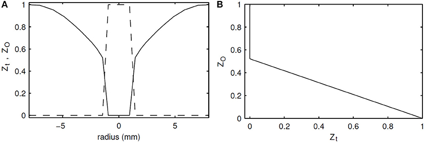
Figure 3. Initial profiles of Z_O (solid) and Z_t (dashed) in radial direction (A), and against each other (B).

$\begin{array}{ll}{Z}_O=\frac{T_0-T_{0,min}}{T_{0,max}-T_{0,min}}& (6)\end{array}$

$\begin{array}{ll}\rho \frac{\partial (Z_O)}{\partial t}+\rho u_i\frac{\partial (Z_O)}{\partial x_i}=\frac{\partial }{\partial x_i}\left(\frac{\lambda }{L{e}_{Z_O}{c}_p}\frac{\partial (Z_O)}{\partial x_i}\right)& (7)\end{array}$

$\begin{array}{ll}L{e}_{Z_O}=1& (8)\end{array}$

With the introduction of Z_O, the species mass fractions and temperature can be represented as $Y_i=Y_i(Z_t,Z_O,{{Y}}_1,{{Y}}_2),T=T(Z_t,Z_O,{{Y}}_1,{{Y}}_2)$, where ${{Y}}_1$ is the first progress variable representing the pre-ignition chemistry, and ${{Y}}_2$ is the second progress variable representing the oxidation chemistry in the MuSt-FGM context.

The definition and selection of Z_O as the control variable representing the oxidizer is similar to what Ihme et al. have used, where they defined an oxidizer split, which would model the effects of the outermost air shroud as well (Ihme and Pitsch, 2008). However, unlike in their study, in this work Z_O was varied within the coflow during the flamelet generation process, and the outermost air shroud part was ignored. The Z_O definition used here is also very similar to the second mixture fraction from the work of Sarras et al. (2014), which is defined as a scaled oxygen mass fraction. However, they further included enthalpy deficit as an extra control variable, and thus represented the species mass fractions as $Y_i=Y_i(Z_1,Z_2,{Y},\Delta h)$. In their case, the temperature variation in the coflow cannot uniquely represent the oxygen variation, and thus the addition of enthalpy deficit as an extra control variable is reasonable.

In order to create the required flamelets, Z_O values corresponding to experimental data points were selected, and 1D autoigniting flame calculations were performed using the composition and temperature data corresponding to each Z_O value as the boundary condition for the oxidizer side. The composition at the fuel side was kept constant as 50% hydrogen and 50% methane by volume. It was observed that at some lower Z_O values, autoignition does not happen because the oxidizer temperature is too low. In Figure 4, the selected Z_O values for which autoignition occurs are shown. The smallest Z_O value which autoignites is 0.710, which corresponds to the oxidizer temperature of 1009 K; and the largest Z_O value which does not autoignite is 0.664, which corresponds to the oxidizer temperature of 962 K. Having non-autoigniting Z_O values poses two problems: the first one is that the MuSt-FGM tables for the second stage (oxidation) at those Z_O values simply cannot be generated, due to the lack of autoignition. The second issue is that even though compositions corresponding to low Z_O values cannot autoignite by themselves, when the ignition occurs at higher Z_O values, heat and species would diffuse into the lower Z_O regions and could trigger ignition. To be able to model such an ignition triggering, and to be able to create tables at lower Z_O values, additional measures have to be taken.

FIGURE 4

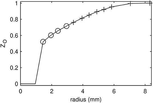
Figure 4. Selected Z_O values with autoignition occurring (plus) and not occurring (circle).

To solve this problem, Ma and Roekaerts used a smaller strain rate than what they used by default, and later switched to the extinguishing flamelet approach (Ma and Roekaerts, 2016). In the current case, however, even for strain rates as low as 1 s⁻¹, autoignition could not be obtained for the lower Z_O values. Furthermore, since this case is an autoigniting one overall, utilizing extinguishing flamelets for every composition is not representative of the system. Using extinguishing flamelets for the non-igniting compositions and autoigniting flamelets for the igniting compositions would cause discontinuity in the tables.

In this work, several methods are proposed to tackle this problem. They are outlined one-by-one in the following subsections.

2.1. Method 1–2D Flamelets

A possible solution to non-igniting oxidizer points problem is to use 2D flamelets like in Hasse and Peters' work (Hasse and Peters, 2005), where they applied it to model one oxidizer and two fuel streams in Diesel engine combustion. In the current study, instead of solving the case in flamelet coordinates, a simulation was performed in 2D physical space, and converted into flamelet coordinates subsequently (x, y, t → Z_t, Z_O and PVs). The temperature, Z_O and Z_t profiles of this simulation are given in Figure 5, where the top part is the oxidizer with temperature gradient, and the bottom part is the fuel. Open outflow boundary conditions were given on all boundaries, and zero initial velocity was defined in the domain. The transient evolution of species and temperature was calculated. As can be seen in Figure 5, Z_t is varied in y-coordinate, Z_O is varied in x-coordinate, and changes in the progress variables are represented by the time coordinate. While the temperature rises with time due to chemical progress, Z_t and Z_O only diffuse. By using 2D flamelets, the diffusion of heat and species from higher Z_O regions to lower Z_O regions is also included, which means that the ignition of lower Z_O values triggered by higher Z_O values can be modeled, and lower Z_O points pose no problem for the table generation.

FIGURE 5

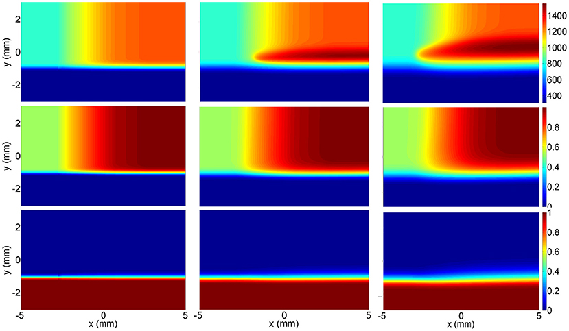
Figure 5. Temperature (Top), Z_O (Middle), and Z_t (Bottom) fields for the 2D flamelet generation simulation at t = 0.0, 1.0, 3.0 ms from left to right.

2.2. Method 2–Forced Ignition

A different approach to solving the problem of non-autoigniting flamelets would be to ignite them artificially. This can be achieved by mixing the initial composition of the non-autoigniting cases with the steady burning composition of the same case by an appropriate ratio, and then letting this artificial mixture to ignite. Note that even though these low Z_O compositions cannot autoignite, when initialized using an already burning solution, steady burning solutions can be obtained. The initial composition is obtained by purely mixing the fuel and oxidizer, and it constitutes the first flamelet of the MuSt-FGM table for that Z_O value. The artificial mixture becomes the second flamelet, and the transient solution from the artificial mixture toward steady solution constitute the rest of the flamelets. To describe the process step by step:

• By initializing the solution with an already burning case, obtain a steady burning solution of a non-autoigniting Z_O point.

• By mixing the steady burning solution of that non-autoigniting Z_O point with its initial state, obtain an artificial mixture that can autoignite by itself. This step is shown in Equations (9) and (10), where Y_new, Y_st and Y_in represent the species mass fraction of the artificial mixture, steady solution and initial mixture, respectively, and h represents the enthalpy with the same notation of the subscripts.

• By trial and error, find the minimum weight m in Equations (9) and (10), which can provide a mixture that can autoignite.

• Using the initial mixing state, artificially created mixture, and the time evolution of the autoigniting case from the artificial mixture until the steady burning solution; create MuSt-FGM tables.

$\begin{array}{ll}{Y}_{new}=m·Y_{st}+(1-m)·Y_{in}& (9)\end{array}$

$\begin{array}{ll}{h}_{new}=m·h_{st}+(1-m)·h_{in}& (10)\end{array}$

This approach is called as “Forced Ignition” in the remaining of the text. The idea behind this approach is to find the minimum weight m where the originally non-autoigniting composition can take off by itself in terms of ignition, and tabulate this autoignition region. Any flamelet which has lower precursor values than the threshold flamelet will quench and not lead to ignition. During an FGM run, if the diffusion of precursor species and heat from an autoigniting Z_O value are high enough to reach this threshold, then the composition at non-autoigniting Z_O will be able to sustain ignition. If the diffusion levels are lower and not continuous, then they will not be sufficient to cause an ignition.

To explain the flamelet creation process in the forced ignition approach more clearly, flamelets from an originally non-autoigniting Z_O value are given in Figure 6. The blue curve represents the initial mixing line, which does not autoignite by itself. By initializing the field from an already burning solution, a steady burning solution for this Z_O value can be obtained, and it is represented with the black curve. Later, the solutions represented by the blue and black curves were mixed by different ratios and then it was checked whether this new solution could autoignite by itself. The mixture that could autoignite with a minimum contribution from the initial mixture solution (min blue/black ratio, so to say) is shown with the red curve in the figure. The red curve, which was also called as artificial mixture so far, will be referred to as “forcing flamelet” from here on. The autoigniting flamelets obtained from the forcing flamelet were stored to create the MuSt-FGM tables, and they are represented with the gray curves in Figure 6. While creating MuSt-FGM tables, the source terms at the forcing flamelet were set to the same source terms as the initial mixing line (blue curve), because otherwise any increase in progress variable would result in a significant source term during MuSt-FGM run. This is caused by the large gap between the blue and red curves, the linear interpolation used in the lookup procedure, and the non-linear relation between progress variables and their source terms.

FIGURE 6

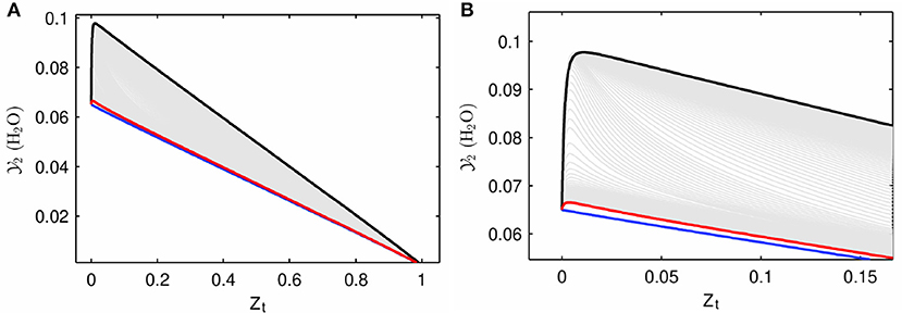
Figure 6. Flamelets created with forced ignition approach. Blue line is the initial mixture, black line is the steady burning solution, and the red line is the mixture of the two which then autoignites and generates flamelets represented with gray lines. This case is for Z_O = 0.664, with a weight m = 0.05. (A,B) Show different Z_t ranges of the same figure.

2.3. Method 3–Default Method

The third approach to the non-autoigniting Z_O points issue is to perform no additional treatment, and leave the non-autoigniting flamelets as they are. Since each progress variable represent a different stage in the MuSt-FGM approach, even though the mixture would not ignite, some pre-ignition chemistry happens regardless and thus can be parameterized by ${{Y}}_1$. As a result, the first lookup table would be non-empty, and the lookup would proceed using only the first table. The implementation of this approach is straightforward, but it misses the conditions where the diffused heat and species from the autoignited compositions would ignite the non-autoigniting compositions. This approach is referred to as “Default Method” in the rest of the text.

Figure 7 shows two sample MuSt-FGM tables for the first (pre-ignition) stage. Figure 7A is from an autoigniting Z_O value, and it is seen that the maximum value for ${{Y}}_1$ and its source term reach ~3 × 10⁻⁵ and 0.035, respectively. Whereas it is seen from Figure 7B, which is from a non-autoigniting Z_O value, that both the source term and maximum value for ${{Y}}_1$ are orders of magnitude lower. This is expected because of the lack of autoignition. However, the table shown in Figure 7B is still usable in a MuSt-FGM calculation as the source terms are very small but non-zero.

FIGURE 7

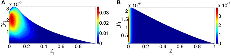
Figure 7. MuSt-FGM first stage table samples for the default method. (A) Is an example of an autoigniting Z_O value (Z_O = 0.710), and (B) is an example of a non-autoigniting Z_O value (Z_O = 0.664). Contour values represent the source term of ${{Y}}_1$. Note the difference in the range of ${{Y}}_1$ values and source terms.

2.4. Method 4–Extrapolation

The final approach for the problem of non-autoigniting Z_O values is to remove those flamelets from the MuSt-FGM table generation all together, and to perform an extrapolation for those compositions during the MuSt-FGM simulations using the autoigniting compositions. For all the variables that are looked up from the tables, linear extrapolation is adapted.

3. Results

3.1. 1D Results

As a first validation step, comparing the results of different modeling approaches with the detailed chemistry case in 1D is reasonable, because the capability of the models to represent the chemistry and diffusion in the absence of turbulence can be verified. In 1D simulations, the initial profiles of Z_O and Z_t as seen in Figure 3 are provided as initial conditions, no velocity is induced, and transient interaction of thermal/molecular diffusion and chemistry is calculated. Therefore this calculation is not a counter-flow flamelet simulation. In the detailed chemistry case and in the flamelet generation, DRM19 reaction mechanism (Kazakov and Frenklach, 1994), which includes 21 species and 84 reactions, was used.

The extrapolation approach failed to give any results as the computations diverged after only a few time steps. This is because the lowest Z_O value (Z_O = 0.514) is the one closest to the fuel, and therefore the whole region between the fuel and oxidizer is being extrapolated (see Figure 3). In addition, the extrapolation step is very large, from Z_O = 0.710 to Z_O = 0.514, while the range of Z_O values for which the MuSt-FGM tables exist is from Z_O = 0.710 to Z_O = 1.0. This introduces a large error in the lookup procedure of many crucial variables, which leads to a quick divergence in the computations.

From the 1D calculation results, spatially averaged heat release rate and the maximum ${{Y}}_2=Y_{{\mathrm{\text{H}}}_2\mathrm{\text{O}}}$ in the whole computational domain are shown in Figure 8. These two variables give a good indication of when the ignition happens, and how fast and intense the oxidation reactions take place. The ignition delay times are also given in Table 2 for all the simulated cases. As seen in Figure 8 and Table 2, the forced ignition and default table cases predict the ignition delay fairly well, with an error of about 4% for both cases compared to the detailed chemistry case. The accuracy of the same cases in predicting the peak of the average heat release rate is less, with an error of about 20%. On the other hand, the 2D flamelet table case completely misses the ignition delay, and performs worse in terms of the peak average heat release rate. It is worth investigating why the 2D flamelet table performs so poorly.

FIGURE 8

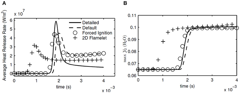
Figure 8. Evolution of average heat release rate (A) and maximum ${{Y}}_2$ in the whole domain (B) in 1D calculations with detailed chemistry, default table, forced ignition table, and 2D flamelet table.

TABLE 2

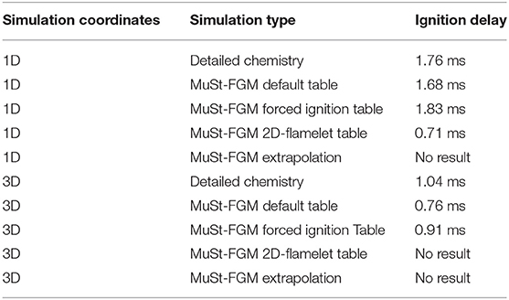
Table 2. Ignition delay times for different cases.

When the progress variable source terms for the first flamelets were checked for the 2D flamelet case at non-autoigniting Z_O values, it was seen that they were at sufficient levels to autoignite by themselves, as shown in Figure 9. It is seen that even though the source term for ${{Y}}_2$ at the first flamelet of Z_O = 0.664 case is not as high as in Z_O = 0.710 case, it is still much larger than its counterpart created with the default table option. This level of source term is sufficient to lead to autoignition. The reason for this high source term can be explained as follows: During the 2D flamelet simulation, higher Z_O values ignite and ${{Y}}_1$ values increase orders of magnitude, and then ${{Y}}_1$ diffuses into lower (non-autoigniting) Z_O values. This creates source terms at lower Z_O values and triggers ignition, as intended with the 2D flamelet approach. However, these source terms are also tabulated at lower progress variable values, i.e., close to the initial mixing line, and cause lower Z_O values to autoignite during an FGM simulation. This is an unintended consequence, because the goal is not to cause lower Z_O compositions to autoignite, but to let them sustain the ignition triggered by diffusion. Since lower Z_O values are closest to the fuel in physical space, this error causes the 2D flamelet case to fail in terms of ignition delay prediction.

FIGURE 9

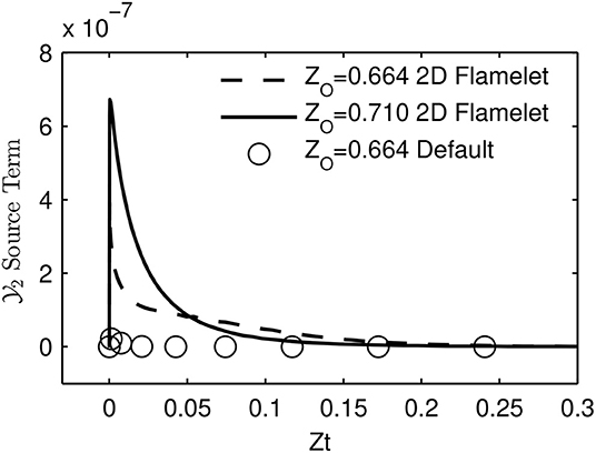
Figure 9. Source term of ${{Y}}_2$ at the first flamelet for different cases.

The default case can predict the ignition delay well because no extra treatment is performed and thus no artificial source term is induced, and in the forced ignition case the artificial source term is removed by setting the source terms at the forcing flamelet same as in the initial mixing line. However, it should be mentioned that part of the reason why extra treatment is performed for non-autoigniting compositions is to be able to capture the effects of triggered ignition at those compositions with the help of diffusion from autoigniting regions. These effects are more visible in the turbulent cases, because the turbulence helps the entrainment of hot parts of the oxidizer with fuel. It is also worth mentioning that judging by the success of ignition delay prediction, it can be concluded that Z_O represents the variation in the oxidizer temperature and resulting chemistry changes well.

To check why peak average heat release rate is lower in the MuSt-FGM cases, the distribution of the heat release rate in the Z_O coordinate is investigated. In Figure 10, this distribution for each case when the peak average heat release rate happens is given. It can be seen that location and distribution of the heat release rate in Z_O space is well captured in the forced ignition case compared to the detailed chemistry case, whereas the default case predicts a heat release at higher Z_O values. This is reasonable because the default case does not have any second stage table (and thus considerable heat release) at lower Z_O values. It is also seen that both MuSt-FGM cases predict the maximum heat release rate correctly, but the heat release rate remains high for a wider range of Z_O values in the detailed chemistry case, which explains the difference in the peak average heat release rates. This might be because the tables are generated using a constant strain rate of 200 s⁻¹, which does not represent the situation for this 1D simulation, where there is only diffusion transport. Nevertheless, the actual goal is to simulate the 3D cases properly, and because it is necessary to entrain the hot parts of the oxidizer and bring them into contact with the fuel to get ignition in the 3D case, flamelets generated with a strain rate is a better option.

FIGURE 10

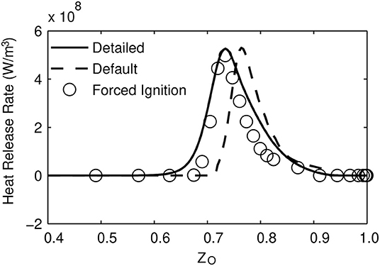
Figure 10. Heat release rate at different Z_O values. The values are taken from the time when the peak average heat release rate occurs for each case.

3.2. 3D Results

As in 1D simulations, average heat release rate and maximum ${{Y}}_2$ are calculated and shown in Figure 11 to make a first comparison between the detailed chemistry and MuSt-FGM. Again the ignition delay times are given in Table 2 as well. Note that since the 2D flamelet case performs poorly for the 1D case, it was not used further in the 3D simulations. The forced ignition case predicts the ignition delay with an error of 12% compared to the detailed chemistry case, which is a decent prediction given the complex structure of the case with preferential diffusion, temperature variations and turbulence. The default case does not perform that well, with the error increasing to 30%. Both MuSt-FGM cases over-predict the maximum increase of ${{Y}}_2$ by about 25%, which is a considerable error. It is also noteworthy that the ignition delay drops by a factor of two compared to the 1D simulations due to the turbulent entrainment, and this effect can be captured with MuSt-FGM cases without any extra treatment.

FIGURE 11

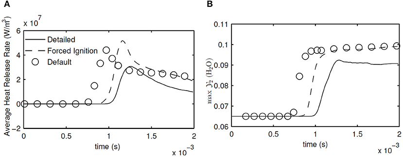
Figure 11. Evolution of average heat release rate (A) and maximum ${{Y}}_2$ in the whole domain (B) in 3D DNS calculations with detailed chemistry and 3D MuSt-FGM with default and forced ignition tables.

Looking at the average heat release rates, it is seen that both MuSt-FGM cases over-predict the peak values compared to the detailed chemistry case. For the forced ignition case, the error for the prediction of the peak average heat release rate is 68%, whereas for the default case it is 43%. Especially for the forced ignition case, the error is at unacceptable levels. In addition to the peak values, also the end value of the average heat release rate is over-estimated by both MuSt-FGM cases. However, it should also be mentioned that the initial increasing slope and the final decreasing slope in time for the average heat release rate are captured rather well with the forced ignition case. As for the maximum ${{Y}}_2$ prediction, the peak value throughout the simulation is over-predicted by 10% by both cases.

When the reasons for early ignition and high heat release rates for the MuSt-FGM cases are investigated, it is seen that the preferential diffusion-curvature interactions are playing a role. This interaction can be summarized as follows: flame curvature enhances or lessens the effects of preferential diffusion (Pitz et al., 2014), this causes a scatter of species in the composition space, this scatter is interpreted as progress in the FGM context, and as a result higher than actual heat release rates are retrieved from the FGM tables. To demonstrate how this interaction affects the distribution in the composition space, the scatter of ${{Y}}_2$ before the ignition (at t = 0.9 ms) is shown in Figure 12. In the MuSt-FGM context, this effect is even more intensified, because the scatter in ${{Y}}_2$ would cause a premature lookup from the second stage table, which would cause even higher heat release rates retrieved.

FIGURE 12

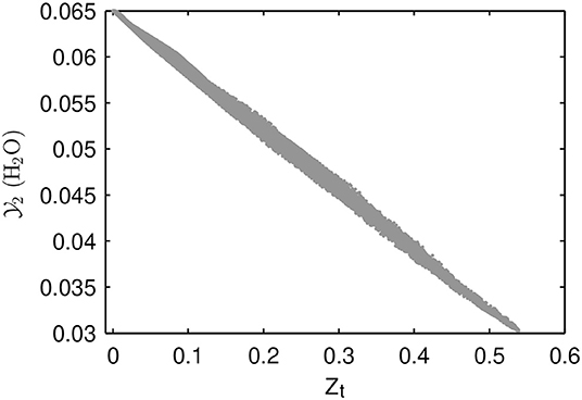
Figure 12. Distribution of ${{Y}}_2$ for the 3D detailed chemistry case at t = 0.9 ms. Note the wide scatter despite almost unity Lewis number of ${{Y}}_2$ (${\text{Le}}_{{{Y}}_2}=0.98$).

In order to demonstrate how the error due to the scatter of species reflects in the actual MuSt-FGM run, contour plots of heat release rate from the detailed chemistry and forced ignition case are shown in Figure 13. The time chosen for each case is when the peak average heat release rate occurs, and the slice in z-direction is chosen as where the maximum heat release rate happens. It is seen that the detailed chemistry case has a more spotty ignition only at the bottom side, whereas the MuSt-FGM case with forced ignition table has a distributed ignition region both at the top and bottom sides. It should also be pointed out that while the average heat release rate differs in two cases by 68%, the difference in maximum heat release rate is 25%, which further supports that the over-prediction of the average heat release rate is because the MuSt-FGM cases lack the variations caused by the scatter of the species.

FIGURE 13

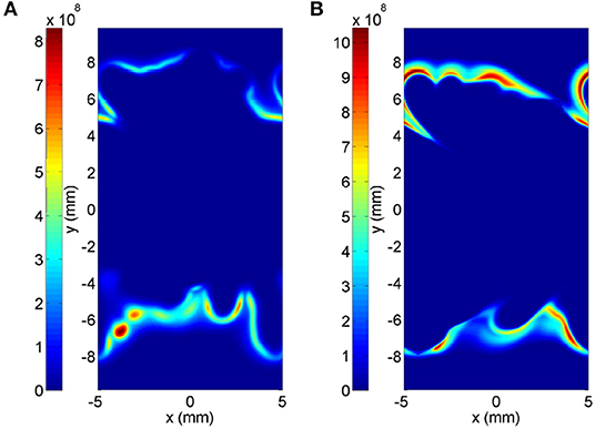
Figure 13. Heat release rate contours (in W/m³) for the detailed chemistry case (A) and the MuSt-FGM forced ignition table case (B), at the time when the peak average heat release rate occurs (t = 1.25 ms and t = 1.16 ms, respectively), and at the z-coordinate where the maximum heat release rate occurs. Please note the difference in color scales.

4. Conclusions

In this study, temperature and oxygen variations in the oxidizer of the Adelaide JHC burner were modeled in the MuSt-FGM context. A new passive variable was defined based on the normalized temperature values, coined as Z_O, and used as the extra control variable. Unsteady counter-flow simulations were performed for each Z_O point to create the necessary flamelets for MuSt-FGM table generation. However, it was realized that not all the compositions in the oxidizer can autoignite. To solve this problem, four approaches were proposed; (1) 2D flamelet creation, (2) helping the non-autoigniting compositions to ignite by mixing with the steady burning solution, (3) simply performing nothing extra and using only the first table (pre-ignition chemistry) of the non-autoigniting regions, (4) not using the non-autoigniting Z_O points in the table generation and applying an extrapolation for those regions. The following conclusions can be drawn from the results and analyses:

• Judging from 1D simulation results, Z_O is a good control variable definition to model the variations in the oxidizer.

• For the current case, creating flamelets from a physical 2D flame simulation did not work well, due to the highly diffusive precursors creating source terms at mixing lines of non-autoigniting Z_O points.

• Extrapolation toward non-autoigniting Z_O values caused the simulations to quickly diverge.

• Although 3D MuSt-FGM with the default table performed well in the 1D simulation, the prediction of the ignition delay as well as the heat release rate deteriorated considerably in the 3D DNS computations.

• 3D MuSt-FGM with the forced ignition case performed better for the ignition delay prediction. However, investigation of the results made it clear that the curvature-preferential diffusion interactions are important for this case.

Although there are open points for improvement such as the inclusion of the curvature-preferential diffusion interactions; considering the difficulty of the investigated MILD combustion case with preferential diffusion, turbulence and the temperature variations; the overall modeling performance for the MuSt-FGM approach can be regarded as successful. Compared to the detailed chemistry case, the ignition delay and the general trend of the average heat release rate are captured fairly well, although the peak value of the average heat release rate is considerably over-predicted.

Data Availability Statement

The datasets generated for this study are available on request to the corresponding author.

Author Contributions

MG has performed the simulations and written the article. As the Ph.D. supervisors, JO and PG have guided the research and provided feedback on the manuscript. JO has conceived and directed the research.

Funding

The Ph.D. project, out of which this study was conducted, had been funded by Dutch Technology Foundation (STW, now part of NWO), under the project name Clean Combustion of Future Fuels and project number 10766.

Conflict of Interest

The authors declare that the research was conducted in the absence of any commercial or financial relationships that could be construed as a potential conflict of interest.

Acknowledgments

Authors wish to thank Prof. Bassam Dally for generously providing the experimental data from the JHC experiments performed in his lab. This study is the result of a project funded by Dutch Technology Foundation (STW, now part of NWO). Computational power provided at the Dutch National Supercomputer, Cartesius, is greatly acknowledged.

References

Abtahizadeh, E., Sepman, A., Hernández-Pérez, F., van Oijen, J., Mokhov, A., de Goey, P., et al. (2013). Numerical and experimental investigations on the influence of preheating and dilution on transition of laminar coflow diffusion flames to mild combustion regime. Combust. Flame 160, 2359–2374. doi: 10.1016/j.combustflame.2013.05.020

CrossRef Full Text | Google Scholar

Afarin, Y., and Tabejamaat, S. (2013). The effect of fuel inlet turbulence intensity on h2/ch4 flame structure of mild combustion using the les method. Combust. Theory Model. 17, 383–410. doi: 10.1080/13647830.2012.742570

CrossRef Full Text | Google Scholar

Albin, T., da Franca, A. A., Varea, E., Kruse, S., Pitsch, H., and Abel, D. (2015). “Potential and challenges of MILD combustion control for gas turbine applications,” in Active Flow and Combustion Control 2014. Notes on Numerical Fluid Mechanics and Multidisciplinary Design. Vol. 127. ed. R. King (Cham: Springer).

Google Scholar

Barlow, R., Frank, J., Karpetis, A., and Chen, J.-Y. (2005). Piloted methane/air jet flames: transport effects and aspects of scalar structure. Combust. Flame 143, 433–449. doi: 10.1016/j.combustflame.2005.08.017

CrossRef Full Text | Google Scholar

Bastiaans, R., Somers, L., and de Lange, H. (2001). “Dns of non-premixed combustion in a compressible mixing layer, using simple chemistry,” in Modern Simulation Strategies for Turbulent Flow, ed B. Geurts (Philadelphia, PA: RT Edwards), 247–261.

Google Scholar

Cabra, R., Myhrvold, T., Chen, J., Dibble, R., Karpetis, A., and Barlow, R. (2002). Simultaneous laser raman-rayleigh-lif measurements and numerical modeling results of a lifted turbulent h2/n2 jet flame in a vitiated coflow. Proc. Combust. Inst. 29, 1881–1888. doi: 10.1016/S1540-7489(02)80228-0

CrossRef Full Text | Google Scholar

Cavaliere, A., and de Joannon, M. (2004). Mild combustion. Prog. Energy and Combust. Sci. 30, 329–366. doi: 10.1016/j.pecs.2004.02.003

CrossRef Full Text | Google Scholar

Chen, Z., Reddy, V., Ruan, S., Doan, N., Roberts, W., and Swaminathan, N. (2017). Simulation of mild combustion using perfectly stirred reactor model. Proc. Combust. Inst. 36, 4279–4286. doi: 10.1016/j.proci.2016.06.007

CrossRef Full Text | Google Scholar

Christo, F., and Dally, B. B. (2005). Modeling turbulent reacting jets issuing into a hot and diluted coflow. Combust. Flame 142, 117–129. doi: 10.1016/j.combustflame.2005.03.002

CrossRef Full Text | Google Scholar

Dally, B., Masri, A., Barlow, R., and Fiechtner, G. (1998). Instantaneous and mean compositional structure of bluff-body stabilized nonpremixed flames. Combust. Flame 114, 119–148.

Google Scholar

Dally, B. B., Karpetis, A., and Barlow, R. S. (2002). Structure of turbulent non-premixed jet flames in a diluted hot coflow. Proc. Combust. Inst. 29, 1147–1154. doi: 10.1016/S1540-7489(02)80145-6

CrossRef Full Text | Google Scholar

De Joannon, M., Sorrentino, G., and Cavaliere, A. (2012). MILD combustion in diffusion-controlled regimes of hot diluted fuel. Combust. Flame 159, 1832–1839. doi: 10.1016/j.combustflame.2012.01.013

CrossRef Full Text | Google Scholar

de Lange, H. (2007). Acoustic upwinding for sub-and super-sonic turbulent channel flow at low Reynolds number. Int. J. Numer. Meth. Fl. 55, 205–223. doi: 10.1002/fld.1446

CrossRef Full Text | Google Scholar

De, A., Oldenhof, E., Sathiah, P., and Roekaerts, D. (2011). Numerical simulation of Delft-jet-in-hot-coflow (DJHC) flames using the eddy dissipation concept model for turbulence–chemistry interaction. Flow Turbul. Combust. 87, 537–567. doi: 10.1007/s10494-011-9337-0

CrossRef Full Text | Google Scholar

Derudi, M., and Rota, R. (2011). Experimental study of the mild combustion of liquid hydrocarbons. Proc. Combust. Inst. 33, 3325–3332. doi: 10.1016/j.proci.2010.06.120

CrossRef Full Text | Google Scholar

Doan, N. A. K., Swaminathan, N., and Minamoto, Y. (2018). Dns of mild combustion with mixture fraction variations. Combust. Flame 189, 173–189. doi: 10.1016/j.combustflame.2017.10.030

CrossRef Full Text | Google Scholar

Donini, A., Martin, S., Bastiaans, R., van Oijen, J., and de Goey, L. (2013). “Numerical simulations of a premixed turbulent confined jet flame using the flamelet generated manifold approach with heat loss inclusion,” in Proceedings of the ASME Turbo Expo 2013: Turbine Technical Conference and Exposition (San Antonio, TX). doi: 10.1115/GT2013-94363

CrossRef Full Text | Google Scholar

Duwig, C., Li, B., Li, Z., and Aldén, M. (2012). High resolution imaging of flameless and distributed turbulent combustion. Combust. Flame 159, 306–316. doi: 10.1016/j.combustflame.2011.06.018

CrossRef Full Text | Google Scholar

Duwig, C., Stankovic, D., Fuchs, L., Li, G., and Gutmark, E. (2007). Experimental and numerical study of flameless combustion in a model gas turbine combustor. Combust. Sci. Technol. 180, 279–295. doi: 10.1080/00102200701739164

CrossRef Full Text | Google Scholar

Evans, M., Medwell, P., Wu, H., Stagni, A., and Ihme, M. (2017). Classification and lift-off height prediction of non-premixed mild and autoignitive flames. Proc. Combust. Inst. 36, 4297–4304. doi: 10.1016/j.proci.2016.06.013

CrossRef Full Text | Google Scholar

Fiorina, B., Baron, R., Gicquel, O., Thevenin, D., Carpentier, S., and Darabiha, N. (2003). Modelling non-adiabatic partially premixed flames using flame-prolongation of ildm. Combust. Theory Model. 7, 449–470. doi: 10.1088/1364-7830/7/3/301

CrossRef Full Text | Google Scholar

Gicquel, O., Darabiha, N., and Thévenin, D. (2000). Liminar premixed hydrogen/air counterflow flame simulations using flame prolongation of ildm with differential diffusion. Proc. Combust. Inst. 28, 1901–1908. doi: 10.1016/S0082-0784(00)80594-9

CrossRef Full Text | Google Scholar

Göktolga, M. U., van Oijen, J. A., and de Goey, L. P. H. (2015). 3D DNS of MILD combustion: a detailed analysis of heat loss effects, preferential diffusion, and flame formation mechanisms. Fuel 159, 784–795. doi: 10.1016/j.fuel.2015.07.049

CrossRef Full Text | Google Scholar

Göktolga, M. U., van Oijen, J. A., and de Goey, L. P. H. (2017). Modeling MILD combustion using a novel multistage FGM method. Proc. Combust. Inst. 36, 4269–4277. doi: 10.1016/j.proci.2016.06.004

CrossRef Full Text | Google Scholar

Groot, G. R. A. (2003). Modelling of Propagating Spherical and Cylindrical Premixed Flames. Ph.D. thesis, Technische Universiteit Eindhoven, Eindhoven.

Google Scholar

Hasse, C., and Peters, N. (2005). A two mixture fraction flamelet model applied to split injections in a di diesel engine. Proc. Combust. Inst. 30, 2755–2762. doi: 10.1016/j.proci.2004.08.166

CrossRef Full Text | Google Scholar

Ihme, M., and Pitsch, H. (2008). Modeling of radiation and nitric oxide formation in turbulent nonpremixed flames using a flamelet/progress variable formulation. Phys. Fluids 20:055110. doi: 10.1063/1.2911047

CrossRef Full Text | Google Scholar

Ihme, M., and See, Y. C. (2011). Les flamelet modeling of a three-stream mild combustor: analysis of flame sensitivity to scalar inflow conditions. Proc. Combust. Inst. 33, 1309–1317. doi: 10.1016/j.proci.2010.05.019

CrossRef Full Text | Google Scholar

Ihme, M., Zhang, J., He, G., and Dally, B. (2012). Large-eddy simulation of a jet-in-hot-coflow burner operating in the oxygen-diluted combustion regime. Flow Turbul. Combust. 89, 449–464. doi: 10.1007/s10494-012-9399-7

CrossRef Full Text | Google Scholar

Kazakov, A., and Frenklach, M. (1994). DRM19 Reaction Mechanism. Available online at: http://www.me.berkeley.edu/drm/ (accessed August 06, 2015).

Kruse, S., Kerschgens, B., Berger, L., Varea, E., and Pitsch, H. (2015). Experimental and numerical study of mild combustion for gas turbine applications. Appl. Energy 148, 456–465. doi: 10.1016/j.apenergy.2015.03.054

CrossRef Full Text | Google Scholar

Kulkarni, R. M., and Polifke, W. (2013). LES of Delft-jet-in-hot-coflow (DJHC) with tabulated chemistry and stochastic fields combustion model. Fuel Process. Technol. 107, 138–146. doi: 10.1016/j.fuproc.2012.06.015

CrossRef Full Text | Google Scholar

Lammel, O., Stohr, M., Kutne, P., Dem, C., Meier, W., and Aigner, M. (2012). Experimental analysis of confined jet flames by laser measurement techniques. Jour. Eng. Gas Turbines Power 134, 041506–041515. doi: 10.1115/1.4004733

CrossRef Full Text | Google Scholar

Lele, S. K. (1992). Compact finite difference schemes with spectral-like resolution. J. Comput. Phys. 103, 16–42.

Google Scholar

Li, P., Mi, J., Dally, B., Wang, F., Wang, L., Liu, Z., et al. (2011). Progress and recent trend in mild combustion. Sci. China Technol. Sci. 54, 255–269. doi: 10.1007/s11431-010-4257-0

CrossRef Full Text | Google Scholar

Ma, L., and Roekaerts, D. (2016). Modeling of spray jet flame under mild condition with non-adiabatic fgm and a new conditional droplet injection model. Combust. Flame 165, 402–423. doi: 10.1016/j.combustflame.2015.12.025

CrossRef Full Text | Google Scholar

Mendez, L. A., Tummers, M., van Veen, E., and Roekaerts, D. (2015). Effect of hydrogen addition on the structure of natural-gas jet-in-hot-coflow flames. Proc. Combust. Inst. 35, 3557–3564. doi: 10.1016/j.proci.2014.06.146

CrossRef Full Text | Google Scholar

Minamoto, Y., Dunstan, T., Swaminathan, N., and Cant, R. (2013). DNS of EGR-type turbulent flame in mild condition. Proc. Combust. Inst. 34, 3231–3238. doi: 10.1016/j.proci.2012.06.041

CrossRef Full Text | Google Scholar

Minamoto, Y., Swaminathan, N., Cant, S. R., and Leung, T. (2014). Morphological and statistical features of reaction zones in MILD and premixed combustion. Combust. Flame 161, 2801–2814. doi: 10.1016/j.combustflame.2014.04.018

CrossRef Full Text | Google Scholar

Moin, P., and Mahesh, K. (1998). Direct numerical simulation: a tool in turbulence research. Annu. Rev. Fluid Mech. 30, 539–578.

Google Scholar

Oldenhof, E., Tummers, M., Van Veen, E., and Roekaerts, D. (2011). Role of entrainment in the stabilisation of jet-in-hot-coflow flames. Combust. Flame 158, 1553–1563.

Google Scholar

Perpignan, A. A., Rao, A. G., and Roekaerts, D. J. (2018). Flameless combustion and its potential towards gas turbines. Prog. Energy Combust. Sci. 69, 28–62. doi: 10.1016/j.apenergy.2017.02.010

CrossRef Full Text | Google Scholar

Peters, N. (1984). Laminar diffusion flamelet models in non-premixed turbulent combustion. Prog. Energy and Combust. Sci. 10, 319–339. doi: 10.1016/0360-1285(84)90114-X

CrossRef Full Text | Google Scholar

Pierce, C. D., and Moin, P. (2004). Progress-variable approach for large-eddy simulation of non-premixed turbulent combustion. J, Fluid Mechan. 504, 73–97. doi: 10.1017/S0022112004008213

CrossRef Full Text | Google Scholar

Pitz, R. W., Hu, S., and Wang, P. (2014). Tubular premixed and diffusion flames: effect of stretch and curvature. Prog. Energy Combust. Sci. 42, 1–34. doi: 10.1016/j.pecs.2014.01.003

CrossRef Full Text | Google Scholar

Poinsot, T. J., and Lelef, S. (1992). Boundary conditions for direct simulations of compressible viscous flows. J. Comput. Phys. 101, 104–129.

Google Scholar

Sarras, G., Mahmoudi, Y., Arteaga Mendez, L., van Veen, E., Tummers, M., and Roekaerts, D. (2014). Modeling of turbulent natural gas and biogas flames of the delft jet-in-hot-coflow burner: Effects of coflow temperature, fuel temperature and fuel composition on the flame lift-off height. Flow Turbul. Combust. 93, 607–635. doi: 10.1007/s10494-014-9555-3

CrossRef Full Text | Google Scholar

Sepman, A. V., Abtahizadeh, S. E., Mokhov, A. V., van Oijen, J. A., Levinsky, H. B., and de Goey, L. P. H. (2013b). Numerical and experimental studies of the NO formation in laminar coflow diffusion flames on their transition to MILD combustion regime. Combust. Flame 160, 1364–1372. doi: 10.1016/j.combustflame.2013.02.027

CrossRef Full Text | Google Scholar

Sepman, A. V., Mokhov, A., and Levinsky, H. (2013a). Spatial structure and NO formation of a laminar methane-nitrogen jet in hot coflow under MILD conditions: a spontaneous raman and LIF study. Fuel 103, 705–710. doi: 10.1016/j.fuel.2012.10.010

CrossRef Full Text | Google Scholar

Somers, L. M. T. (1994). The simulation of flat flames with detailed and reduced chemical models. Ph.D. thesis, Technische Universiteit Eindhoven, Eindhoven.

Google Scholar

Swaminathan, N. (2019). Physical insights on mild combustion from dns. Front. Mechan. Eng. 5:59. doi: 10.3389/fmech.2019.00059

CrossRef Full Text | Google Scholar

Tang, Z., Ma, P., Li, Y.-L., Tang, C., Xing, X., and Lin, Q. (2010). Design and experiment research of a novel pulverized coal gasifier based on flameless oxidation technology. Proc. CSEE 30, 50–55.

Google Scholar

van Oijen, J. (2013). Direct numerical simulation of autoigniting mixing layers in MILD combustion. Proc. Combust. Inst. 34, 1163–1171. doi: 10.1016/j.proci.2012.05.070

CrossRef Full Text | Google Scholar

Van Oijen, J., Bastiaans, R., and De Goey, L. (2007). Low-dimensional manifolds in direct numerical simulations of premixed turbulent flames. Proc. Combust. Inst. 31, 1377–1384. doi: 10.1016/j.proci.2006.07.076

CrossRef Full Text | Google Scholar

van Oijen, J., and de Goey, L. (2000). Modelling of premixed laminar flames using flamelet-generated manifolds. Combust. Sci. Technol. 161, 113–137. doi: 10.1080/00102200008935814

CrossRef Full Text | Google Scholar

Vasavan, A., de Goey, P., and van Oijen, J. (2018). Numerical study on the autoignition of biogas in moderate or intense low oxygen dilution nonpremixed combustion systems. Energy Fuels 32, 8768–8780. doi: 10.1021/acs.energyfuels.8b01388

PubMed Abstract | CrossRef Full Text | Google Scholar

Wünning, J., and Wünning, J. (1997). Flameless oxidation to reduce thermal NO-formation. Prog. Energy Combust. Sci. 23, 81–94.

Google Scholar