Evaluation of Modeling Approaches for MILD Combustion Systems With Internal Recirculation

Introduction

The simultaneous requirements of thermal efficiency, fuel flexibility, and low pollutant emission are the main drivers for the development of innovative combustion-based systems. Several concepts were developed in the last decades, to achieve lower temperatures of the oxidation region and avoid the formation of several classes of pollutants. In particular, a number of combustion concepts based on the internal or external dilution and/or preheating of main reactants were proposed. They include flameless oxidation (Wünning and Wünning, 1997), colorless combustion (Khalil and Gupta, 2017), high-temperature air combustion (HiTAC) (Rafidi and Blasiak, 2006), and moderate or intense low-oxygen dilution (MILD). Examples of implementation of these technologies include furnaces, boilers, and gas turbines.

MILD combustion plays today a crucial role in the development of flexible, efficient, and nonpolluting technologies. Notably, its feeding conditions allow the establishment of a distributed reaction zone, with almost uniform temperatures in the combustion chamber, absence of a visible flame, very low levels of noise and fluctuations, absence of soot particles, and negligible NO_x and CO emissions (Cavaliere and de Joannon, 2004). In the last decades, strong attention was given to the turbulent combustion modeling of such processes. In fact, the unique thermochemical features related to the turbulence–chemistry interaction have led to the development of new modeling paradigms or to the adaptation of the ones already used for conventional conditions (De and Dongre, 2015). In such systems, the flue gases' recirculation decreases the oxygen level of the reactant mixture, thus slowing down the kinetic rates in such a way that the characteristic chemical timescales approach the mixing timescales; that is, the Damköhler number is close to unity (Özdemir and Peters, 2001). Due to such modifications of the reaction zone, appropriate turbulence/chemistry interaction models need to be developed (Frassoldati et al., 2010). In particular, detailed kinetic mechanisms should be considered to correctly capture the thermochemical variable distributions (temperature and main species fields) and pollutant emissions in particular.

The complexity of MILD reaction structures has pushed the development of a number of approaches for Reynolds-averaged Navier–Stokes (RANS) (Galletti et al., 2007) and large-eddy simulations (LES) (Duwig et al., 2007), which can be divided into flamelet-like and finite-rate approaches, depending on the assumptions made with respect to the accessible reaction state space (Pope, 2013).

Flamelet-based models allow us to include detailed chemistry effects at an affordable computational cost, as the chemical state space is calculated in a preprocessing step, and it is then accessed during the actual simulation via a number of scalars (typically the mixture fraction and a progress variable) that parameterize the chemical state space (Pierce and Moin, 2001, 2004). In this context, tabulated chemistry techniques such as the flamelet-generated manifold (FGM) (Van Oijen and De Goey, 2000) and flamelet progress variable (FPV) (Pierce and Moin, 2001, 2004) techniques have acquired a key role in the combustion community, and their effectiveness has been demonstrated for a number of problems and configurations. Recently, Abtahizadeh et al. (2015) showed that the canonical structure used for tabulation strongly influences the representation of MILD combustion in jet in hot coflow (JHC) configurations. Such results were confirmed by Sorrentino et al. (2018a), for a cyclonic flow burner. A relevant challenge in FGM/FPV approaches is to include the effects of exhaust gas recirculation in the lookup tables, to properly represent the dilution and heat loss effects (Lamouroux et al., 2014). The inclusion of additional variables in the tabulation procedure is a very demanding task and can lead to expensive computational fluid dynamics (CFD) simulations due to the increased manifold dimensionality (from 3D or 4D to 6D).

Reaction rate-based approaches have been also proposed in the literature and applied to MILD conditions. Among them, it is worth mentioning the eddy dissipation concept (EDC) (Magnussen, 2005) and the partially stirred reactor (PaSR) model, originally proposed by Chomiak (1990). Both models divide each grid cell into two regions: the reacting structures, modeled as ideal reactors, and the surrounding fluid mixture. The main difference between the two approaches lies in the estimation of the reacting structures' volume fraction. In EDC, the latter is solely based on the turbulence properties of the flow, obtained by means of an energy cascade model (Magnussen, 2005). In PaSR, the reacting fraction explicitly depends on both the mixing and chemical timescales. Recently, the PaSR model was used to simulate the Adelaide JHC, using both RANS (Ferrarotti et al., 2019) and LES (Ihme and See, 2011), with very satisfactory results. Despite the encouraging progress in the use of reactor-based models for MILD combustion, there are still open questions related to the general applicability of the concept to different configurations. To this end, the availability of experimental data in MILD conditions is key.

Both the Adelaide and Delft JHC configurations (Dally et al., 2002; Oldenhof et al., 2011) mimic MILD conditions by feeding diluted and hot streams to the coflow, impacting directly the system characteristic chemical timescale. This simplified configuration makes it possible to perform optical diagnostics and deliver high-fidelity experimental data that are crucial for model development. However, in industrial MILD configurations, the distributed conditions are a consequence of the internal aerodynamic recirculation and the modification of the local mixing timescales. Closed furnaces operating in MILD conditions allow, in principle, challenging of the ability of turbulent combustion models to appropriately capture turbulence/chemistry interactions. For instance, Ferrarotti et al. (2018) applied the PaSR model for a quasi-industrial burner fed with natural gas, showing the relevance of both mixing and chemical timescales as well as of the comprehensiveness of the chemical mechanism.

The availability of experimental data in furnace configurations is generally limited due to the presence of an enclosure. In addition, available data in MILD conditions are limited to narrow operative conditions. Based on such considerations, the present study reports the investigation of a novel cyclonic burner (Sorrentino et al., 2018b). A methane-fired small-scale burner was employed, and detailed internal temperature measurements were used to characterize the local thermal field. Experimental temperature measurements were used to validate two different modeling paradigms, a tabulated chemistry approach, FGM, and a reactor-based model, PaSR. The comparison was carried out for two experimental configurations, involving standard air and diluted air as the oxidizer stream. The main aim of the paper is to identify current potential and limitations of turbulent combustion closures for the investigation of more complex MILD combustion configurations.

Experimental Test Case

The geometrical features and characteristics of the cyclonic burner used in this article to mimic MILD combustion conditions have been reported in previous works (de Joannon et al., 2017; Ferrarotti et al., 2019; Sabia et al., 2019; Sorrentino et al., 2019). In the following, the key features of the device are discussed.

It consists of a lab-scale combustor (20 * 20 cm² of square section and a height of 5 cm) where a cyclonic and toroidal flow field is established through two couples of coaxial oxidant/fuel inlet jets located in an antisymmetric configuration. In Figure 1, a sketch of the burner midplane, the feeding configuration, and the position of the thermocouples are shown. Oxidizer and fuel injection pipes are placed 2 and 4.5 cm from the lateral walls, respectively. The flue gas exit is placed at the top-central side. In the present manuscript, methane was used as a fuel and air as oxidizer.

FIGURE 1

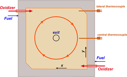
Figure 1. Sketch of the midplane of the combustion chamber.

MILD conditions are ensured thanks to the strong internal recirculation of burned products that stabilizes locally a distributed ignition. Such a microscopic feature of MILD combustion corresponds macroscopically to reduced temperature gradients (high levels of temperature uniformity) with very low pollutant emissions.

Two shielded N-type thermocouples can be moved along the y-direction. The lateral one is placed 0.02 m from the wall, whereas the central thermocouple is located 0.01 m from the confinement.

External ceramic preheating ovens were used to fix the boundary conditions in terms of external temperature, thus controlling the heat flux through the surroundings. The burner was built with a three-layer structure of alumina, a thick layer of heat-insulating material, and an outer shell of stainless steel 310s. The oxidant flow passes through heaters, to keep fixed the inlet temperature to the desired values (T_in).

In the present work, the two experimental configurations illustrated in Table 1 were investigated. In the first case, the fuel (pure methane) was injected at the environmental temperature (300 K) with a jet velocity of 15.8 m/s, while the oxidizer (preheated air) was fed at a fixed preheating level of 1,000 K (T_in) and with a jet velocity of 17.8 m/s. The inlet equivalence ratio was kept constant at the stoichiometric value. Moreover, a mean overall heat loss flux at walls (Q_W) was estimated by means of thermocouples placed on outer and inner surfaces of the walls to be equal to 13 kW/m², for the investigated conditions. In the second case, the air stream was diluted with 90% N₂ by volume. The equivalence ratio was kept to stoichiometric value, and the inlet temperatures were as in case 1; the fuel jet velocity was 15.8 m/s, while the oxidizer jet was 54.17 m/s.

TABLE 1

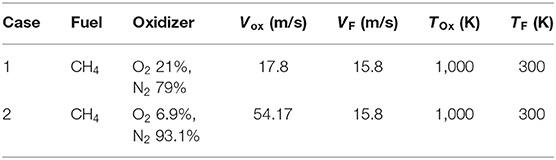
Table 1. List of the conditions investigated in this study.

Modeling Tools

Numerical simulations were carried out using RANS, with the commercial code Ansys Fluent 19.3. The grid was generated with the software Ansys Workbench. A grid independence study was performed using a polyhedral grid with a number of cells ranging from 100 to 400 k. The selected grid consisted of 450 k polyhedral elements. Reynolds stresses were solved using the RNG k–ε turbulence model with swirl-dominated flow corrections to take into account the high swirl level in the combustor. The discrete ordinate (DO) radiation model was used, while the radiation properties of the reacting mixture are accounted for with the weighted-sum-of-gray-gases (WSGG) model, using the coefficients proposed by Smith et al. (1982).

For the turbulence–chemistry interaction, PaSR and FGM models were adopted. As with other reactor-based models, the computational cell in PaSR is split into two zones, the reaction structures and the surrounding fluid. The overall reaction progress is determined by the exchange between the two regions. The mass fraction of the reaction zone is estimated, considering both the characteristic chemical and mixing timescales:

$\begin{array}{ll}\kappa =\frac{{\tau }_c}{{\tau }_c+{\tau }_{mix}}& (1)\end{array}$

$\begin{array}{ll}\overline{\stackrel{*}{\omega }}=\kappa \frac{\rho (Y_i^{*}-Y^0)}{{\tau }^{*}}& (2)\end{array}$

A first set of simulations was performed to determine the influence of the kinetic mechanism on the results. The detailed mechanisms GRI2.11 (Bilger et al., 1990; Bowman et al., 1996) and GRI3.0 (Smith et al., 2011), along with the reduced mechanism KEE (Bilger et al., 1990), were used. Then, a sensitivity to the PaSR model parameters was carried out, with special emphasis on the determination of the mixing scale. First, τ_mix was estimated as in Ferrarotti et al. (2018), considering a fraction of the integral timescale κ/ϵ by means of a constant C_mix:

$\begin{array}{ll}{\tau }_{mix,s}=C_{mix}\frac{\kappa }{ϵ}& (3)\end{array}$

Values of C_mix ranging 0.01, 0.1, and 0.5 were considered. Then, a dynamic approach was used, as proposed in Ferrarotti et al. (2019), based on local properties of the flow field. τ_{mix, d} is estimated with the ratio of the mixture fraction variance, Z″², to the mixture fraction dissipation rate, χ:

$\begin{array}{ll}{\tau }_{mix,d}=\frac{\widetilde{Z^{{}^{″}2}}}{\tilde{\chi }}& (4)\end{array}$

The determination of τ_{mix, d} requires the solution of transport equations for $\widetilde{Z^{{}^{″}2}}$ and $\tilde{\chi }$, expressed as

$\begin{array}{ll}\frac{D\rho \widetilde{Z^{{}^{″}2}}}{Dt}=\frac{\partial }{\partial x_j}\left(\rho (D_m+D_t)\frac{\partial \widetilde{Z^{{}^{″}2}}}{\partial x_j}\right)+2\rho D_t{\left(\frac{\partial \tilde{Z}}{\partial x_j}\right)}^2-\rho \tilde{\chi }& (5)\end{array}$

$\begin{array}{l}\frac{D\rho \tilde{\chi }}{Dt}=\frac{\partial }{\partial x_j}\left(\rho (D_m+D_t)\frac{\partial \tilde{\chi }}{\partial x_j}\right)-C_{D_1}\bar{\rho }\frac{\widetilde{{\chi }^2}}{\widetilde{Z^{{}^{″}2}}}-C_{D_2}\bar{\rho }\frac{\tilde{\chi }\widetilde{ϵ}}{\tilde{\kappa }}\\ +C_{P_1}\frac{\tilde{\chi }}{\widetilde{Z^{{}^{″}2}}}{P}_f+C_{P_2}\frac{\tilde{\chi }}{\tilde{\kappa }}{P}_{\kappa }& (6)\end{array}$

where Z is the mixture fraction, D_t is the turbulent diffusivity, $P_f=-2\widetilde{\overline{\rho }{u}_k^{″}{Z}^{″}}(\frac{\partial \tilde{Z}}{\partial x_k})$ is the production of scalar fluctuation, and $P_k=-\widetilde{\overline{\rho }{u}_k^{″}{u}_i^{″}}(\frac{\partial {\tilde{U}}_i}{\partial x_k})$ is the production of turbulent kinetic energy. The set of coefficients C_P1, C_P2, C_D1, C_D2 used is the one proposed in Keehan Ye (2011). The resulting system is solved using an unsteady RANS (URANS) approach.

The PaSR model was benchmarked to the FGM model (Van Oijen and De Goey, 2000). In FGM, 1D flame configurations were employed by means of igniting mixing layer (IML) (Abtahizadeh et al., 2015) and premixed flamelet equations (Van Oijen et al., 2016). The thermochemical quantities were tabulated as functions of the mixture fraction and progress variable. At the CFD runtime, only the transport equations for the mean values and the variances of the controlling variables (in addition to continuity, momentum, and energy) were solved, and all the required parameters were retrieved. Specifically, the main assumptions behind the FGM method are that a turbulent flame can be represented by an ensemble of laminar flames, and the n-dimensional composition space can be replaced by a lower-dimensional manifold (Chen et al., 2018; Sorrentino et al., 2018a). The flamelet equations were computed through the specialized solver Chem1D, developed at the University of Technology of Eindhoven (TU/e) (Somers, 1994). A unity Lewis number assumption was chosen, whereas the GRI3.0 chemical mechanism was used.

Two controlling variables were chosen, a progress variable Y and a mixture fraction Z, to represent the mixing between fuel and oxidizer. Usually, under traditional combustion conditions, the standard FGM model adopts combustion products, such as CO₂ and H₂O, to define the progress variable. Nevertheless, in this work, HO₂ was also included. Indeed, Medwell et al. (2008) stressed the role of precursor species like HO₂ in MILD combustion. Therefore, a combination of H₂O, CO₂, and HO₂ was selected as progress variable to include the effects of both preignition and oxidation chemistry. The general form of the progress variable is

$\begin{array}{ll}Y={\displaystyle \sum _{i=1}^{N_{sp}}}{\alpha }_i{X}_i& (7)\end{array}$

where X_i is the molar fractions and α_i the weight factors of the generic species i, which were optimized to yield a smooth mapping between the state space and the transported variables. In this work, the coefficients α were chosen as α_H2O = 100/W_H2O, α_CO2 = 100/W_CO2, α_HO2 = 1,000/W_HO2, where W_i denotes the molar mass of species i. α_i = 0 for all other species. Moreover, the progress variable was scaled between 0 and 1, to make it independent of the mixture fraction. The controlling variables and the lookup tables were defined by means of Matlab R2019a (The Mathworks Inc., 2019) scripts. Thus, all the thermochemical parameters calculated from flamelet equations were tabulated as a function of Y and Z.

Once defined, the laminar and adiabatic 2D tables were imported on Fluent using the FGM dedicated routine. The effect of the turbulence was considered incrementing the manifold dimension from 2 to 4, using a presumed β – PDF approach (Fiorina et al., 2005). In this way, both the mean values (100 table points) and the variances (11 table points) of Y and Z are considered as controlling variables.

During a simulation, the turbulent transport equations for the mean and variance of the mixture fraction ($\tilde{Z}$ and $\widetilde{Z_{\upsilon }}$, respectively) and for the mean and variance of the progress variable (Ỹ and $\widetilde{Y_{\upsilon }}$, respectively) are solved in addition to the Favre-averaged mass, momentum, and enthalpy conservation equations. The four steady-state transport equations read as follows:

$\begin{array}{ll}\frac{\partial \bar{\rho }{ũ}_j\tilde{Z}}{\partial x_j}=\frac{\partial }{\partial x_j}\left[\left(\bar{\rho }D+\frac{{\mu }_t}{S{c}_t}\right)\frac{\partial \tilde{Z}}{\partial x_j}\right]& (8)\end{array}$

$\begin{array}{ll}\frac{\partial \bar{\rho }{ũ}_jỸ}{\partial x_j}=\frac{\partial }{\partial x_j}\left[\left(\bar{\rho }D+\frac{{\mu }_t}{S{c}_t}\right)\frac{\partial Ỹ}{\partial x_j}\right]+\overline{{\omega }_Y}& (9)\end{array}$

$\begin{array}{l}\frac{\partial \bar{\rho }{ũ}_j\widetilde{Z_{\upsilon }}}{\partial x_j}=\frac{\partial }{\partial x_j}\left[\left(\bar{\rho }D+\frac{{\mu }_t}{S{c}_t}\right)\frac{\partial \widetilde{Z_{\upsilon }}}{\partial x_j}\right]+C_1\frac{{\mu }_t}{S{c}_t}\frac{\partial \tilde{Z}}{\partial x_i}\frac{\partial \tilde{Z}}{\partial x_i}\\ -C_2\bar{\rho }\frac{\tilde{\epsilon }}{\tilde{k}}\widetilde{Z_{\upsilon }}& (10)\end{array}$

$\begin{array}{l}\frac{\partial \bar{\rho }{ũ}_j\widetilde{Y_{\upsilon }}}{\partial x_j}=\frac{\partial }{\partial x_j}\left[\left(\bar{\rho }D+\frac{{\mu }_t}{S{c}_t}\right)\frac{\partial \widetilde{Y_{\upsilon }}}{\partial x_j}\right]+2\frac{{\mu }_t}{S{c}_t}\frac{\partial Ỹ}{\partial x_i}\frac{\partial Ỹ}{\partial x_i}\\ -C_2\bar{\rho }\frac{\tilde{\epsilon }}{\tilde{k}}\widetilde{Y_{\upsilon }}+\overline{2Y^{{}^{″}}{\omega }_Y}& (11)\end{array}$

In the equations above, $\bar{\rho }$ is the mean density, ũ_j is the mean velocity vector, D is the molecular diffusion coefficient, μ_t is the turbulent viscosity, Sc_t is the turbulent Schmidt number, $\overline{{\omega }_Y}$ is the mean chemical source term of the progress variable, C₁ and C₂ are the modeling constants, $\tilde{k}$ is the mean turbulent kinetic energy, and $\tilde{\epsilon }$ is the mean dissipation rate.

Since the lookup tables were created from adiabatic flamelets, heat losses were not included in the manifold and, therefore, only considered in the CFD simulations. The accuracy of this approach is then related to the accuracy associated with the inclusion of the enthalpy in Fluent once the adiabatic tables are imported. In particular, the software includes enthalpy by freezing the species in the adiabatic flamelets and recalculating the temperatures and the progress variable source terms with the enthalpy.

Results and Discussion

Case 1 (described in Table 1) is first considered. Figure 2 shows the temperature profiles along the lateral thermocouple obtained with the PaSR model in combination with three chemical mechanisms, the GRI3.0, GRI2.11, and KEE, using a C_mix of 0.1. It can be observed that the temperature profiles are almost superimposed, with differences never exceeding 4%. Based on this observation, it was decided to keep the KEE mechanism for the subsequent simulations, to reduce the associated computational time.

FIGURE 2

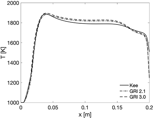
Figure 2. Case 1 PaSR results along the lateral thermocouple. Comparison of KEE, GRI2.11, and GRI3.0 mechanisms for C_mix = 0.1.

In Figures 3A,B, the numerical predictions were compared to the experiments in terms of temperature profiles along the central and lateral thermocouples. It can be observed how the FGM method shows a good agreement with the experiments for the central thermocouple (Figure 3A). In particular, the temperature profile predicted by FGM is quite homogeneous, and it well captures the temperature peaks in the near-wall regions, only slightly overestimating it by about 50 K. However, when looking at the lateral position, FGM strongly overpredicts the experimental trend of about 200°, with a very localized peak close to the inlet zone (x < 0.06 m). Such a strong difference between the central and lateral positions suggests that the model predicts a very early ignition after injection, contrary to the experimental observations suggesting distributed reaction conditions. The fact that the reaction and heat release region predicted by FGM are very localized also explains why FGM well captures the central thermal field, the progress variable being unitary in this area and heat transfer dominating the flow features. The inability of FGM to capture the initiation and extension of the reaction region can be related to the absence of a controlling variable, taking into account the internal dilution by the combustion products, in the construction of the lookup table.

FIGURE 3

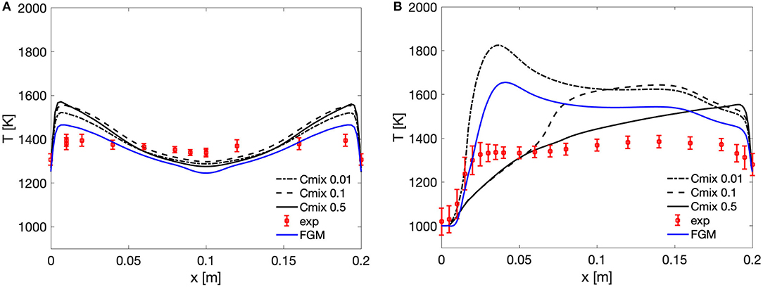
Figure 3. Case 1 comparison between FGM and PaSR with C_mix of 0.01, 0.1, and 0.5 and experimental values along the central and lateral thermocouples. (A) Central thermocouple profiles. (B) Lateral thermocouple profiles.

Figures 3A,B also show the PaSR predictions for different values of the C_mix constant. As a remainder, increasing C_mix increases the mixing timescale value. The temperature profiles obtained with C_mix values of 0.01, 0.1, and 0.5 clearly show the strong sensitivity of the model to the estimation of the mixing scale. In particular, decreasing C_mix impacts the mean reaction rate in two ways, via the reacting structure fraction κ and the residence time in the reacting structures (taken equal to the mixing time). When C_mix is reduced, representative of a condition of intense mixing, the reacting fraction κ (Equation 1) is increased, indicating that the whole computational cells evolve toward a perfectly stirred reactor. At the same time, the denominator in Equation (2) decreases, thus impacting directly the mean reaction rate, which is increased. A close observation of Figures 3A,B suggests that a C_mix value of 0.5 is the most appropriate choice for the case under investigation, in agreement with previous results (Ferrarotti et al., 2018, 2019). Nevertheless, when looking at the centerline thermocouple (Figure 3A), all PaSR simulations underpredict the temperature near the outlet zone (0.06 < x < 0.14 m), while overestimating the temperature level on the sides. The shapes of the PaSR temperature profile clearly indicate that the model can capture the existence of a distributed reaction region, but not to the extent suggested by the experimental measurements, showing a very uniform profile. This is further confirmed by the analysis of Figure 3B, which shows how the PaSR results show a delayed ignition with respect to the experimental data, as the temperature peak reduces and moves downstream of the fuel injection. Increasing C_mix helps to reduce the temperature overpredictions along the thermocouples, although the central thermocouple profile is still not quite well represented, as the maximum temperature is about 150 K higher than the experimental values. Opposed to experimental data, the PaSR simulation still retains two defined reaction zones, which are the cause of the temperature spikes along the central thermocouple profile (Figure 3A).

Interestingly, as C_mix is decreased, FGM and PaSR become more similar. This is explained by the direct impact that the mixing timescale has on the mean reaction rate (Equation 2). As discussed above, a reduction in τ_mix directly impacts $\overline{\stackrel{*}{\omega }}$ and increases it. This is further confirmed by the analysis of the Damköhler number maps presented in Figure 4, showing how the Damköhler in the domain decreases by one order of magnitude as C_mix is decreased from 0.5 to 0.01. As Dα decreases, the reactive zone mass fraction κ (Equation 1) increases, thus increasing the mean reaction rate as well. The combined effects of reducing τ^* and increasing κ in Equation 2 results in the above-mentioned temperature spikes in the C_mix = 0.01 case.

FIGURE 4

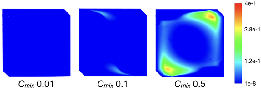
Figure 4. Case 1 Damköhler contours for PaSR static simulations with C_mix of 0.01, 0.1, and 0.5.

One tool that can be helpful to understand the differences between the two models results is the so-called normalized flame index, introduced by Yamashita et al. (1996) and defined by Bray et al. (2005), Domingo et al. (2002), and Knudsen and Pitsch (2009, 2012) as

$\begin{array}{ll}\xi =\frac{\nabla Y_F·\nabla Y_O}{|\nabla Y_F·\nabla Y_O|}& (12)\end{array}$

By definition, the index takes the value of ξ = +1 in premixed flames and ξ = −1 in non-premixed ones. It can be then useful to assess the ability of the model to capture the premixed nature of the combustion process under MILD conditions. Figure 5 shows the contours of the flame index obtained using both the PaSR model, using C_mix = 0.5, and FGM. It can be observed that the two models yield quite different results. With the PaSR case, the non-premixed region is almost exclusively restricted to the injection zone, between x = 0 m and x = 0.05 m; in the rest of the chamber mixing, it occurs effectively before reaction, and the flame index is +1, indicating a premixed region. The same cannot be said about FGM: beside the injection zone, the flame index contour presents four additional regions close to the chamber walls, where the flame index value is −1, thus indicating a non-premixed flame structure. This can be ascribed to the very assumptions of the FGM formulation used in the present work and specifically to the lack of a dilution parameter to describe the mixing between fresh reactants and combustion products before reaction, thus resulting in the temperature overprediction shown in Figure 3B.

FIGURE 5

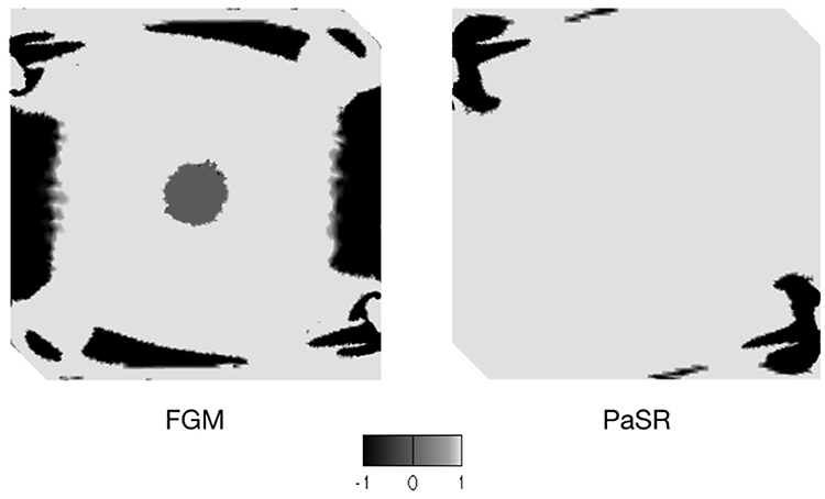
Figure 5. Case 1 flame index contours for FGM and PaSR static simulations.

The PaSR results presented above clearly show that the model can potentially capture the distributed features of MILD combustion. At the same time, the estimation of the mixing timescale has a key role in the structure of the reaction zone and the temperature levels. In particular, it is clear that the use of a simple approach for τ_mix, based on a fraction of the integral mixing scale, is not appropriate to describe the complexity of turbulence–chemistry interactions in the system under investigation. Therefore, the dynamic model (Equations 5, 6) was used for the same configuration, to assess whether the scalar time of a (non)reactive scalar could represent an appropriate choice. It should be stressed here that a large uncertainty is associated to the determination of this scalar dissipation rate via Equation 6 (Knudsen and Pitsch, 2009): the coefficients used in such an equation are the result of a calibration on simple-flow configurations (Ferrarotti et al., 2019) and might be inadequate for the complex flow under investigation. The results of the dynamic model using the coefficient by Keehan Ye (2011) show results very close to the C_mix = 0.5 case. As shown in Figures 6A,B, the temperature profiles along the lateral thermocouple are almost identical, with the exception of the zone between x = 0.07 m and x = 0.15 m, where the dynamic model yields slightly higher temperatures and a flatter profile. The dynamic model yields slightly lower maximum temperatures in the reaction zone along the central thermocouple and lower temperatures around x = 0.1 m. Figure 7 shows the contour of the equivalent C_mixeq for the dynamic case. The equivalent C_mixeq is calculated as follows (Ferrarotti et al., 2019):

$\begin{array}{ll}{C}_{mi{x}_{eq}}=\frac{{\tau }_{mix,d}}{\raisebox{1ex}{$k$}\!\left/ \!\raisebox{-1ex}{$\epsilon $}\right.}& (13)\end{array}$

where τ_mix,d is the mixing timescale for the dynamic approach defined in section Modeling Tools. It is possible to see in Figure 7 how the average value of C_mixeq in the reaction zone is close to 0.5, thus explaining the agreement of the static and dynamic cases. However, the dynamic model still cannot capture the initial ignition of the system. The reason for such deficiency can be explored by means of sophisticated models for turbulent mixing, using for instance detached eddy simulation (DES) and LES.

FIGURE 6

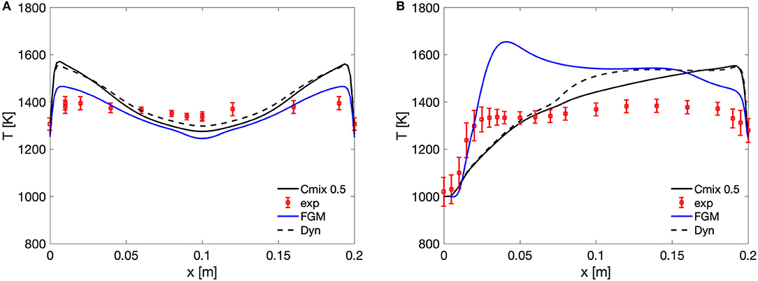
Figure 6. Case 1 static and dynamic PaSR results compared to experimental values along the central and lateral thermocouples. (A) Central thermocouple profiles. (B) Lateral thermocouple profiles.

FIGURE 7

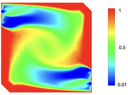
Figure 7. Case 1 C_mixeq contour for the PaSR dynamic model.

The FGM and static PaSR with C_mix = 0.5 were then tested for the experimental conditions of case 2 (Table 1). With respect to case 1, both FGM and PaSR better capture the experimental trends. This is probably due to the dilution of the oxidizer stream, which causes the smoothing of the reaction process, resulting in a homogeneous temperature distribution. Figure 8 shows that, while FGM better predicts the temperature peak along the central thermocouple, the PaSR model enhances the temperature predictions in the ignition region along the lateral thermocouple, although it overpredicts the peak temperature by about 100 K. With respect to the central thermocouple, the PaSR model slightly overpredicts the peak temperature, while FGM underpredicts the observed values in the central region, that is, close to the outlet.

FIGURE 8

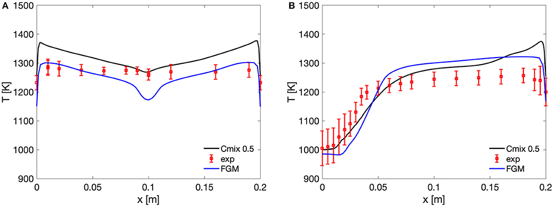
Figure 8. Case 2 FGM and static PaSR with C_mix = 0.5 results compared to experimental values along the central and lateral thermocouples. (A) Central thermocouple profiles. (B) Lateral thermocouple.

Conclusions

Numerical simulations of a lab-scale MILD cyclonic burner were carried out with two different turbulence–chemistry interaction closures, FGM and PaSR, in a RANS framework. The numerical results were compared to the available experimental temperature measurements, in the ignition zone and in the burner midplane.

The main findings can be summarized as follows:

• The thermocouple profiles overall are better represented by the PaSR model results; while the FGM model yields slightly better results along the central thermocouple, the PaSR model better captures the typical slow ignition of MILD systems in both operative conditions.

• A C_mix of 0.5 seems to be the better fit for these combinations of fuel and operative conditions. The a posteriori analysis of the dynamic PaSR model equivalent C_mixeq shows that for the static model, C_mix = 0.5 is the optimal value for the present cases.

• The analysis of the flame index reveals that the two models determine quite different mixing behaviors: FGM results show that the reaction regions all exhibit non-premixed behavior, while on the other hand the PaSR model determines mostly a premixed environment. As can be expected, the two different behaviors reflect on the temperature profiles, as the different ways mixing is handled between the two models strongly affect the computation of the reaction rates. Further experimental investigations of the cyclonic burner could then be key to determining which of the two numerical approaches would be the better option.

• With the increase of the dilution level in case 2, the differences in the predictive capabilities of the two models lower; the dilution slows down the reaction process, yielding a more homogeneous temperature field, thus explaining the lack of a strong temperature overprediction in the reactive regions by the FGM model as in case 1.

Even though PaSR results are overall better than those of FGM, both closures display some limitations which can be ascribed to the turbulent mixing models employed in RANS computations. For this reason, LES analysis of the same burner will be carried out, to explore the effect of turbulent mixing modeling accuracy on the results.

Data Availability Statement

The datasets generated for this study are available on request to the corresponding author.

Author Contributions

GC and GS provided experimental results and FGM results. RA and MF provided PaSR results and wrote first draft of the manuscript. GC wrote sections of the manuscript. All authors contributed to manuscript revision and approved the submitted version and contributed conception and design of the study.

Conflict of Interest

The authors declare that the research was conducted in the absence of any commercial or financial relationships that could be construed as a potential conflict of interest.

Acknowledgments

This project has received funding from the European Research Council (ERC) under the European Union's Horizon 2020 research and innovation program under grant agreement no. 714605. The first and third authors wish to thank the Fonds de la Recherche Scientifique (FNRS) Belgium for financing their research. This article is based upon work from COST Action SMARTCATs (CM1404), supported by COST (European Cooperation in Science and Technology, http://www.cost.eu).

References

Abtahizadeh, E., de Goey, P., and van Oijen, J. (2015). Development of a novel flamelet-based model to include preferential diffusion effects in autoignition of CH4/H2 flames. Combust. Flame 162, 4358–4369. doi: 10.1016/j.combustflame.2015.06.015

CrossRef Full Text | Google Scholar

Bilger, R. W., Stårner, S. H., and Kee, R. J. (1990). On reduced mechanisms for methane/air combustion in nonpremixed flames. Combus. Flame 80, 135–149. doi: 10.1016/0010-2180(90)90122-8

CrossRef Full Text | Google Scholar

Bowman, C. T., Hanson, R. K., Davidson, D. F., Gardiner W. C. Jr Lissianski, V., Smith, G. P., et al. (1996). Available online at: http://combustion.berkeley.edu/gri-mech/releases.html

Google Scholar

Bray, K., Domingo, P., and Vervisch, L. (2005). Role of the progress variable in models for partially premixed turbulent combustion. Combust. Flame 141, 431–437. doi: 10.1016/j.combustflame.2005.01.017

CrossRef Full Text | Google Scholar

Cavaliere, A., and de Joannon, M. (2004). Mild combustion. Progr. Energy Combust. Sci. 30, 329–366. doi: 10.1016/j.pecs.2004.02.003

CrossRef Full Text | Google Scholar

Chen, Z. X., Doan, N. A. K., Lv, X. J., Swaminathan, N., Ceriello, G., Sorrentino, G., et al. (2018). Numerical study of a cycloinic combustor under Moderate or Intense Low-Oxygen Dilution conditions using non-adiabatic tabulated chemistry. Energy Fuels 32, 10256–10265. doi: 10.1021/acs.energyfuels.8b01103

CrossRef Full Text | Google Scholar

Chomiak, J. (1990). Combustion: A Study in Theory, Fact and Application. Abacus Press/Gorden and Breach Science Publishers.

Google Scholar

Dally, B. B., Karpetis, A. N., and Barlow, R. S. (2002). Structure of turbulent non-premixed jet flames in a diluted hot coflow. Proc. Combust. Inst. 29, 1147–1154. doi: 10.1016/S1540-7489(02)80145-6

CrossRef Full Text | Google Scholar

de Joannon, M., Sabia, P., Sorrentino, G., Bozza, P., and Ragucci, R. (2017). Small size burner combustion stabilization by means of strong cyclonic recirculation. Proc. Combust. Inst. 36, 3361–3369. doi: 10.1016/j.proci.2016.06.070

CrossRef Full Text | Google Scholar

de Joannon, M., Sorrentino, G., and Cavaliere, A. (2012). MILD combustion in diffusion-controlled regimes of hot diluted fuel. Combust. Flame 159, 1832–1839. doi: 10.1016/j.combustflame.2012.01.013

CrossRef Full Text | Google Scholar

De, A., and Dongre, A. (2015). Assessment of turbulence-chemistry interaction models in MILD combustion regime. Flow Turbul. Combust. 94, 439–478. doi: 10.1007/s10494-014-9587-8

CrossRef Full Text | Google Scholar

Domingo, P., Vervisch, L., and Bray, K. (2002). Partially premixed flamelets in LES of non-premixed turbulent combustion. Combust. Theory Model. 6, 529–551. doi: 10.1088/1364-7830/6/4/301

CrossRef Full Text | Google Scholar

Duwig, C., Stankovic, D., Fuchs, L., Li, G., and Gutmark, E. (2007). Experimental and numerical study of flameless combustion in a model gas turbine combustor. Combust. Sci. Technol. 180, 279–295. doi: 10.1080/00102200701739164

CrossRef Full Text | Google Scholar

Ferrarotti, M., Fürst, M., Cresci, E, de Paepe, W., and Parente, A. (2018). Key modeling aspects in the simulation of a quasi-industrial 20 kW moderate or intense low-oxygen dilution combustion chamber. Energy Fuels 32, 10228-10241. doi: 10.1021/acs.energyfuels.8b01064

CrossRef Full Text | Google Scholar

Ferrarotti, M., Li, Z., and Parente, A. (2019). On the role of mixing models in the simulation of MILD combustion using finite-rate chemistry combustion models. Proc. Combust. Inst. 37, 4531–4538. doi: 10.1016/j.proci.2018.07.043

CrossRef Full Text | Google Scholar

Fiorina, B., Gicquel, O., Vervisch, L., Carpentier, S., and Darabiha, N. (2005). Premixed turbulent combustion modleing using tabulated chemistry and PDF. Proc. Combust. Inst. 30, 867–874. doi: 10.1016/j.proci.2004.08.062

CrossRef Full Text | Google Scholar

Frassoldati, A., Sharma, P., Cuoci, A., Faravelli, T., and Ranzi, E. (2010). Kinetic and fluid dynamics modeling of methane/hydrogen jet flames in diluted coflow. Appl. Thermal Eng. 30, 376–383. doi: 10.1016/j.applthermaleng.2009.10.001

CrossRef Full Text | Google Scholar

Galletti, C., Parente, A., and Tognotti, L. (2007). Numerical and experimental investigation of a MILD combustion burner. Combust. Flame 151, 649–664. doi: 10.1016/j.combustflame.2007.07.016

CrossRef Full Text | Google Scholar

Ihme, M., and See, Y. C. (2011). LES flamelet modeling of a three-stream MILD combustor: analysis to sensitivity to scalar inflow conditions. Proc. Combust. Inst. 33, 1309–1317. doi: 10.1016/j.proci.2010.05.019

CrossRef Full Text | Google Scholar

Keehan Ye, I. (2011). Investigation of the Scalar Variance and Scalar Dissipation Rate in URANS and LES. PhD thesis, University of Waterloo, Waterloo, Ontario, Canada.

Google Scholar

Khalil, A. E., and Gupta, A. K. (2017). Towards colorless distributed combustion regime. Fuel 195, 113–122. doi: 10.1016/j.fuel.2016.12.093

CrossRef Full Text | Google Scholar

Knudsen, E., and Pitsch, H. (2009). A general flamelet transformation useful for distinguishing between premixed and non-premixed modes of combustion. Combust. Flame 153, 678–696. doi: 10.1016/j.combustflame.2008.10.021

CrossRef Full Text | Google Scholar

Knudsen, E., and Pitsch, H. (2012). Capabilities and limitations of multi-regime flamelet combustion models. Combust. Flame 159, 242–264. doi: 10.1016/j.combustflame.2011.05.025

CrossRef Full Text | Google Scholar

Lamouroux, J., Ihme, M., Fiorina, B., and Gicquel, O. (2014). Tabulated chemistry approach for diluted combustion regimes with internal recirculation and heat losses. Combust. Flame 161, 2120–2136. doi: 10.1016/j.combustflame.2014.01.015

CrossRef Full Text | Google Scholar

Magnussen, B. F. (2005). “The eddy dissipation concept, a bridge between science and technology,” in ECCOMAS Thematic Conference on Computational Combustion (Lisbon).

Google Scholar

Medwell, P. R., Kalt, P. A. M., and Dally, B. B. (2008). Imaging of diluted turbulent ethylene flames stabilized on a Jet in Hot Coflow (JHC) burner. Combust. Flame 152, 100–113. doi: 10.1016/j.combustflame.2007.09.003

CrossRef Full Text | Google Scholar

Oldenhof, E., Tummers, M. J., Van Veen, E. H., and Roekaerts, D. J. E. M. (2011). Role of entrainment in the stabilisation of jet-in-hot-coflow flames. Combust. Flame 158, 1553–1563. doi: 10.1016/j.combustflame.2010.12.018

CrossRef Full Text | Google Scholar

Özdemir, I. B., and Peters, N. (2001). Characteristics of the reaction zone in a combustor operating at MILD combustion. Exp. Fluids 30, 683–695. doi: 10.1007/s003480000248

CrossRef Full Text | Google Scholar

Pierce, C., and Moin, P. (2001). Progress-Variable Approach for Large-Eddy Simulation Of Turbulent Combustion. Ph.D. Thesis, Mechanical Engineering Dept., Stanford University, Stanford.

Google Scholar

Pierce, C., and Moin, P. (2004). Progress-variable approach for large-eddy simulation of non-premixed turbulent combustion. J. Fluid Mech. 504, 73–97. doi: 10.1017/S0022112004008213

CrossRef Full Text | Google Scholar

Pope, S. (2013). Small scales, many species and the manifold challenges of turbulent combustion. Proc. Combust. Inst. 34:1–31. doi: 10.1016/j.proci.2012.09.009

CrossRef Full Text | Google Scholar

Rafidi, N., and Blasiak, E. (2006). Heat transfer characteristics of HiTAC heating furnace using regenerative burners. Appl. Thermal Eng. 26, 2027–2034. doi: 10.1016/j.applthermaleng.2005.12.016

CrossRef Full Text | Google Scholar

Sabia, P., Sorrentino, G., Bozza, P., Ceriello, G., Ragucci, R., and de Joannon, M. (2019). Fuel and thermal load flexibility of a MILD burner. Proc. Combust. Inst. 37, 4547–4554. doi: 10.1016/j.proci.2018.09.003

CrossRef Full Text | Google Scholar

Smith, G. P., Golden, D. M., Frenklach, M., Moriarty, N. W., Eiteneer, B., Goldenberg, M., et al. (2011). GRI-Mech 3.0. Available online at: http://combustion.berkeley.edu/gri-mech/releases.html (accessed May 20, 2020).

Google Scholar

Smith, T. F., Shen, Z. F., and Friedman, J. N. (1982). Evaluation of coefficients for the weighted sum of gray gases model. J. Heat Transf. 104, 602–608. doi: 10.1115/1.3245174

CrossRef Full Text | Google Scholar

Somers, L. M. T. (1994). The Simulation of Flat Flames With Detailed and Reduced Chemical Models (PhD thesis).

Google Scholar

Sorrentino, G., Ceriello, G., De Joannon, M., Sabia, P., Ragucci, R., Van Oijen, J., et al. (2018a). Numerical investigation of moderate or intense low-oxygen dilution combustion in a cyclonic burner using a flamelet-generated manifold approach. Energy Fuels 32, 10242–10255. doi: 10.1021/acs.energyfuels.8b01099

CrossRef Full Text | Google Scholar

Sorrentino, G., Sabia, P., Bozza, P., Ragucci, R., and de Joannon, M. (2019). Low-NOx conversion of pure ammonia in a cyclonic burner under locally diluted and preheated conditions. Appl. Energy 254:113676. doi: 10.1016/j.apenergy.2019.113676

CrossRef Full Text | Google Scholar

Sorrentino, G., Sabia, P., de Joannon, M., Bozza, P., and Ragucci, R. (2018b). Influence of preheating and thermal power on cyclonic burner characteristics under MILD combustion. Fuel 233, 207–214. doi: 10.1016/j.fuel.2018.06.049

CrossRef Full Text | Google Scholar

The Mathworks Inc. (2019). MATLAB Version 9.6.

Google Scholar

Van Oijen, J. A., and De Goey, L. P. H. (2000). Modelling of premixed laminar flames using flamelet-generated manifolds. Combust. Sci. Technol. 161, 113–137. doi: 10.1080/00102200008935814

CrossRef Full Text | Google Scholar

Van Oijen, J. A., Donini, A., Bastiaans, R. J. M., ten Thije Boonkkamp, J. H. M., and de Goey, L. P. H. (2016). State-of-the-art in premixed combustion modeling using flamelet generated manifolds. Progr. Energy Combust. Sci. 57, 30–74. doi: 10.1016/j.pecs.2016.07.001

CrossRef Full Text | Google Scholar

Wünning, J. A., and Wünning, J. G. (1997). Flameless oxidation to reduce thermal NO formation. Progr. Energy Combust. Sci. 23, 81–94. doi: 10.1016/S0360-1285(97)00006-3

CrossRef Full Text | Google Scholar

Yamashita, H., Shimada, M., and Takeno, T. (1996). A numerical study on flame stability at the transition point of jet diffusion flames. Proc. Combust. Inst. 26, 27–34. doi: 10.1016/S0082-0784(96)80196-2

CrossRef Full Text | Google Scholar