Transient and Steady Sliding Friction of Elastomers: Impact of Vertical Lift

Introduction

It has been well-known that sliding contact of elastomers involves various types of dynamics due to friction. Physical phenomena such as wave propagations (Schallamach, 1971; Barquins, 1985; Rubinstein et al., 2004; Maegawa and Nakano, 2010), wear pattern formations (Schallamach, 1957; Fukahori and Yamazaki, 1994), and nonlinear vibrations (Nakano and Maegawa, 2009; Yamaguchi et al., 2011; Nakano et al., 2019) have attracted the interest of many scientific and engineering researchers. Among various elastomers, rubber is the material that has received the most attention in various practical applications (e.g., tires, seals, and shoes). Since the study done by Grosch (1963) showing the master curve of friction coefficient according to Williams–Landel–Ferry (WLF) theory (Williams et al., 1955), the importance of viscoelasticity has been recognized, and the dependence of the friction coefficient on temperature and velocity has been investigated [e.g., Popov et al. (2018)]. More recently, several swollen polymers showing high elasticity and ultra-low friction (e.g., hydrogels and polymer brushes) have been found (Gong et al., 2001; Nomura et al., 2011), some of which are being developed toward practical applications (Belin et al., 2018; Tadokoro et al., 2020), and their tribological properties have also been discussed in relation to their viscoelastic properties (Mizukami et al., 2019).

To understand the sliding friction of elastomers, various types of modeling methods have been proposed. Among them, those with “viscoelastic foundations” are known to have strong advantages not only of avoiding the difficulties of elastic contact stress theory but also of providing intuitive pictures of how the energy dissipation occurs inside the contact. The first was the extension of the elastic foundation (i.e., the Winkler foundation) from stationary contact problems of thin films to steady sliding contact problems of elastomers (May et al., 1959; Johnson, 1985). Then recently, in the novel framework of the “Method of Dimensionality Reduction” invented by Popov and his colleagues, the modeling method has progressed, enabling us to analyze the true three-dimensional contact with high accuracy (Popov, 2010; Popov and Heß, 2015; Kusche, 2017). For example, Li et al. (2015) numerically and theoretically studied the kinetics of friction coefficient for the sliding contact between a flat elastomer (modeled by a Kelvin–Voigt foundation) and a rough rigid indenter (modeled by a self-affine fractal) under abrupt change in the drive velocity. As a result, they found interesting temporal changes (i.e., jumps and relaxations) of the friction coefficient depending on the drive velocity and the Hurst exponent of the self-affine fractal, under the consideration of quasi-static processes.

Based on the foregoing background, the aim of this study was to find the answer to the following question: What is the minimum requirement for modeling with viscoelastic foundations to describe the transient friction appearing in the onset of sliding between an elastomer and an indenter? In this article, to provide a possible answer in a minimal situation, we consider a simple line contact between a flat elastomer and a cylindrical rigid indenter, focusing on the boundary condition of the rigid indenter in the vertical direction, under the restriction that the elastomer is modeled by the conventional Kelvin–Voigt foundation. Two types of models with different boundary conditions reveal that the vertical dynamics of the rigid indenter strongly affects not only the occurrence of the transient sliding friction but also the characteristics of the steady sliding friction.

Note that the aforementioned idea on the boundary condition in the vertical direction originates from the typical structure of sliding systems under the fluid film lubrication, since when the fluid film lubrication is considered theoretically, it is natural to assume that the “slider” (corresponding to the “indenter” in this study) shifts vertically to find the position to balance with the applied normal load. Also note that in general, it has been known that the friction of elastomers arises by two different mechanisms. One is the “adhesion,” the energy dissipation of which occurs at the contact interface between the elastomer and indenter [i.e., the adhesive friction (e.g., Moore and Geyer (1972))], and the other is the “viscoelasticity,” the energy dissipation of which occurs inside the elastomers [i.e., the hysteresis friction (e.g., Moore and Geyer (1974))]. Although both mechanisms are important and should be interrelated, this study ignores the former and focuses on the latter.

Models

Structures

Figure 1 shows the two types of models for sliding friction of elastomers considered in this study. The left is termed the “fixed indenter (FI) model,” and the right is termed the “movable indenter (MI) model.” They are models describing the two-dimensional sliding contact between a rigid indenter and a viscoelastic foundation in the xz plane, where the x and z axes are taken in the horizontal and vertical directions, respectively.

FIGURE 1

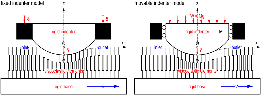
Figure 1. Two types of models for sliding contact between cylindrical rigid indenter and flat elastomer (modeled by viscoelastic foundation). (Left) Fixed indenter (FI) model. (Right) Movable indenter (MI) model.

The rigid indenter (mass per unit width: M) has a cylindrical shape (curvature radius: R), the bottom surface of which contacts with the viscoelastic foundation. In the FI model, the rigid indenter is mounted on the rigid walls, not to be able to move in any direction. In the MI model, on the other hand, the rigid indenter is supported by a frictionless linear bearing, to be able to move only in the vertical direction. Note that the boundary condition of the rigid indenter is the single difference between them.

The viscoelastic foundation consists of an infinite number of viscoelastic elements mounted on a rigid base at regular intervals in the horizontal direction. Every viscoelastic element is a one-degree-of-freedom Kelvin–Voigt element consisting of a vertical spring (stiffness per unit width: k) and a vertical damper (damping coefficient per unit width: c) with the same natural length; as a result, its non-disturbed surface is the horizontal plane z = 0. Note that by using the stiffness per unit area (K) and damping coefficient per unit area (C) of the viscoelastic foundation, k and c are given by k = K/N and c = C/N, respectively, where N is the number of viscoelastic elements per unit length. Also note that here we assume that the upper end of every viscoelastic element makes contact with the rigid indenter surface with no adhesion and with no friction.

Owing to the aforementioned structures, the normal load per unit width (W) of the FI model is determined by the indentation depth δ [i.e., W = W(δ), where δ is constant], while that of the MI model is determined by the gravity [i.e., W = Mg, where g is the gravity constant]. In addition, in both models, the rigid base is driven horizontally at the drive velocity V. Therefore, we can say that the FI model represents a “constant-gap sliding system,” while the MI model represents a “dead-weight sliding system.” Or, we can also say that the FI and MI models represent the two limiting cases corresponding to a “very stiff apparatus” and a “very soft apparatus,” respectively.

Governing Equations

When the rigid indenter penetrates the viscoelastic foundation by δ > 0, the indenter surfaces in the FI and MI models are given by

$\begin{array}{ll}z=h(x)-\delta (\text{FI model})& (1)\end{array}$

$\begin{array}{ll}z=h(x)-\delta (t)(\text{MI model})& (2)\end{array}$

respectively, where t is the time, and h(x) is the indenter shape function:

$\begin{array}{ll}h(x)=\frac{x^2}{2R}& (3)\end{array}$

Let us assume that the ith viscoelastic element at x = x_i(t) makes contact with the indenter surface (see Figure 2). The compression and compression rate of the ith viscoelastic element in the FI model are given by

$\begin{array}{ll}{u}_i(t)=-h(x_i)+\delta (\text{FI model})& (4)\end{array}$

$\begin{array}{ll}{\stackrel{.}{u}}_i(t)=-h^{\prime }(x_i)V(\text{FI model})& (5)\end{array}$

respectively, while in the MI model,

$\begin{array}{ll}{u}_i(t)=-h(x_i)+\delta (t)(\text{MI model})& (6)\end{array}$

$\begin{array}{ll}{\stackrel{.}{u}}_i(t)=-h^{\prime }(x_i)V+\stackrel{.}{\delta }(t)(\text{MI model})& (7)\end{array}$

respectively, where (^·) and (′) are the derivatives with respect to t and x, respectively. Then, as shown in the left of Figure 2, there are four types of local forces acting on the subelement PQR: the normal force f _Ni at P (from the rigid indenter), the restoring force ku_i at Q (from the spring), the damping force $c{\stackrel{.}{u}}_i$ at R (from the damper), and the horizontal constraint force f _Ci (from the spring and damper). Considering that the subelement PQR is massless, we obtain the following force balance equations in the vertical and horizontal directions:

$\begin{array}{ll}k{u}_i+c{\stackrel{.}{u}}_i=f_{\text{N}i}\text{ cos }{\theta }_i& (8)\end{array}$

$\begin{array}{ll}{f}_{\text{C}i}=f_{\text{N}i}\text{ sin }{\theta }_i& (9)\end{array}$

respectively, where

$\begin{array}{ll}\text{tan }{\theta }_i=-h^{\prime }(x_i)& (10)\end{array}$

under –π/2 < θ_i < π/2, and from Equation (8),

$\begin{array}{ll}{f}_{\text{N}i}=\frac{k{u}_i+c{\stackrel{.}{u}}_i}{\text{cos }{\theta }_i}& (11)\end{array}$

Now, as shown in the right of Figure 2, the normal force acts on the rigid indenter at P from the ith viscoelastic element, which is the reaction force of the normal force f _Ni on the left of Figure 2. Therefore, the vertical and horizontal components of the normal force are given by

$\begin{array}{ll}{f}_{zi}=f_{\text{N}i}\text{ cos }{\theta }_i=k{u}_i+c{\stackrel{.}{u}}_i& (12)\end{array}$

$\begin{array}{ll}{f}_{xi}=f_{\text{N}i}\text{ sin }{\theta }_i=-h^{\prime }(x_i)f_{zi}& (13)\end{array}$

respectively. Note that from Equations (9) and (13), the horizontal constraint force is determined as f _Ci = f_xi. Consequently, the total vertical force F_z and total horizontal force F_x acting on the rigid indenter from the viscoelastic foundation are given by

$\begin{array}{ll}{F}_z={{\displaystyle \sum }}_i{f}_{zi}& (14)\end{array}$

$\begin{array}{ll}{F}_x={{\displaystyle \sum }}_i{f}_{xi}& (15)\end{array}$

respectively. Finally, the vertical position of the indenter bottom A in the FI model is given by

$\begin{array}{ll}{z}_{\text{A}}=-\delta (\text{FI model})& (16)\end{array}$

while in the MI model, it is determined by the equation of motion:

$\begin{array}{ll}M{\ddot{z}}_{\text{A}}=F_z-Mg(\text{MI model})& (17)\end{array}$

which determines δ and $\stackrel{.}{\delta }$ in Equations (6) and (7) as follows:

$\begin{array}{ll}\delta (t)=-z_{\text{A }}(t)(\text{MI model})& (18)\end{array}$

$\begin{array}{ll}\stackrel{.}{\delta }(t)=-{\stackrel{.}{z}}_{\text{A}}(t)(\text{MI model})& (19)\end{array}$

Note that when the ith viscoelastic element is not making contact with the indenter surface, it is obvious that f _Ni = 0 and therefore f_zi = f_xi = 0. Then, the compression rate of the non-contacting element is given by

$\begin{array}{ll}{\stackrel{.}{u}}_i=-\frac{u_i}{\tau }(\text{non-contact})& (20)\end{array}$

where τ is the retardation time of the viscoelastic element, defined as

$\begin{array}{ll}\tau =\frac{c}{k}& (21)\end{array}$

or, by using the macroscopic properties of the viscoelastic foundation,

$\begin{array}{ll}\tau =\frac{C}{K}& (22)\end{array}$

Therefore, when the contacting element violates the following condition:

$\begin{array}{ll}{u}_i\ge h^{\prime }(x_i)V\tau (\text{FI model})& (23)\end{array}$

$\begin{array}{ll}{u}_i\ge h^{\prime }(x_i)V\tau +{\dot{z}}_{\text{A}}\tau (\text{MI model})& (24)\end{array}$

it detaches from the rigid indenter surface. Note that the first-order differential equation (20) for the non-contacting element has the following solution:

$\begin{array}{ll}{u}_i(t)=u_i(t_0)\text{ exp}\left(-\frac{t-t_0}{\tau }\right)(\text{non-contact})& (25)\end{array}$

where t₀ is the constant.

FIGURE 2

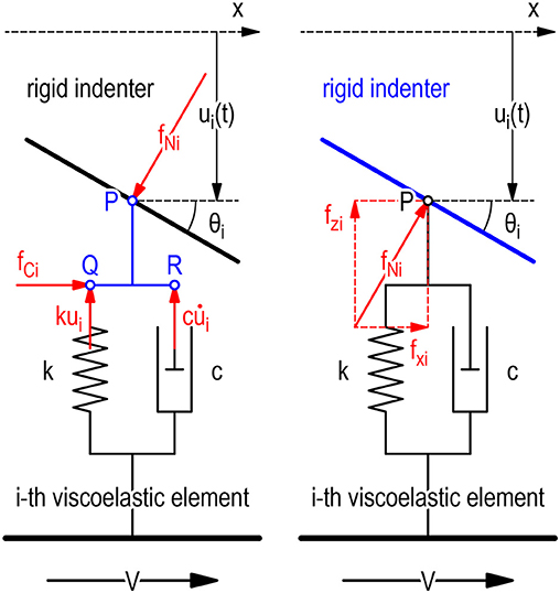
Figure 2. Local forces on the ith viscoelastic (Kelvin–Voigt) element. (Left) Local forces acting on subelement PQR in the ith viscoelastic element. (Right) Local force acting on rigid indenter from the ith viscoelastic element.

Methods

The sets of the governing equations in the previous section were solved numerically for the FI and MI models. To solve the second-order ordinary differential equation (17) for the MI model, the Runge–Kutta method was used, where the time discretization was determined by Δt = 2Δx/V = 2/NV.

Standard parameter values for the numerical simulations are listed in Table 1. Note that both models include six independent parameters (R, K, τ, N, δ, and V in the FI model; R, M, K, τ, N, and V in the MI model). However, since N (= 1/ Δx) is the parameter for the space discretization, the number of essential parameters is five for each model. Also note that if we imagine a “thin” elastic sheet of thickness h = 1 mm as the viscoelastic foundation, it is possible to say that the stiffness per unit area K = 10 GN/m³ corresponds to the effective elastic modulus E ~ Kh = 10 MPa, although it depends strongly on the boundary condition of mounting the elastomer on the rigid base [e.g., Popov (2010)].

TABLE 1

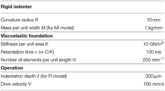
Table 1. Standard parameter values for numerical simulations.

Results

Figure 3 shows the numerical results of temporal changes in representative variables for the FI model (left column) and MI model (right column) under the standard conditions (Table 1). Note that as shown by the blue lines in the top row, the drive velocity was abruptly increased from V = 0 to 100 mm/s at t = 0.

FIGURE 3

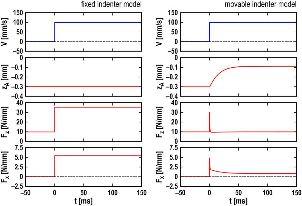
Figure 3. Numerical results for fixed indenter model (Left) and movable indenter model (Right): temporal changes in drive velocity V (top row), indenter position z_A (second row), total vertical force F_z (third row), and total horizontal force F_x (bottom row) under standard conditions (see Table 1 for parameter values).

First, from the results for the FI model, we find that the indenter position provided the initial condition (z_A = −0.3 mm, F_z ~ 10 N/mm, and F_x = 0). Then, F_z and F_x were immediately increased at t = 0 and maintained the increased values (z_A = −0.3 mm, F_z ~ 35 N/mm, and F_x ~ 5 N/mm).

Then, from the results for the MI model, we find that the gravity force provided the same initial condition as that of the previous model. However, the responses were completely different, showing distinct “transient sliding” toward “steady sliding.” The rigid indenter started to move “upward” at t = 0 and then gradually approached z_A ~ −0.1 mm with a time constant in the order of “10 ms” (second row). The response of F_z was spiky: it immediately increased to F_z ~ 30 N/mm at t = 0, then rapidly decreased to F_z ~ 9 N/mm with a time constant in the order of “1 ms,” and gradually returned to F_z ~ 10 N/mm (third row). The response of F_x was also spiky: it immediately increased to F_x ~ 5 N/mm at t = 0, then rapidly decreased to F_x ~ 2 N/mm with the time constant “1 ms,” and gradually approached F_x ~ 1 N/mm with the time constant “10 ms” (bottom row). It should be noted that the response of F_x resembles the typical transition from the static friction to the kinetic friction, although no static friction was considered. This transient behavior will be discussed in the next section.

Figure 4 shows the numerical results of spatiotemporal changes in the contact pressure p(x,t) = Nf _N(x,t) under the same conditions as those of the previous figure, where the abscissa is the horizontal position x, the ordinate is the time t, and the magnitude of p is represented by the shade of the red color. The blue lines show temporal changes in the horizontal positions of the leading and trailing edges of the contact area, denoted by x_LE(t) and x_TE(t), respectively.

FIGURE 4

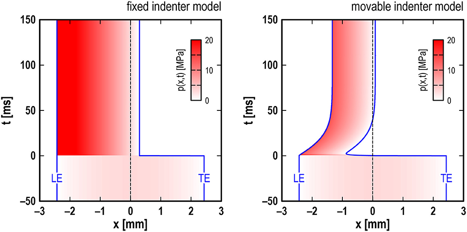
Figure 4. Numerical results for fixed indenter model (Left) and movable indenter model (Right): spatiotemporal changes in contact pressure p(x,t) under standard conditions (see Table 1 for parameter values). LE, leading edge of contact; TE, trailing edge of contact.

First, from the results for the FI model, we again find that the response was not accompanied by any transient processes. Regarding the edges, they were located at x_LE = −2.4 mm and x_TE = 2.4 mm as the initial state. After t = 0, the leading edge maintained the position, while the trailing edge immediately moved to the left to x_TE = 0.3 mm at t = 0 and maintained the position for t > 0 (which is observed as the peeling of the contact area in the outlet side). Regarding the contact pressure, it was symmetric for t < 0, showing the maximum p_max ~ 3 MPa at the contact center and the minimum p_min = 0 at both edges. After t = 0, it showed the maximum p_max > 20 MPa at the leading edge and the minimum p_min = 0 at the trailing edge.

Then, from the results for the MI model, we again find that the response was accompanied by distinct transient processes. Regarding the edges, they were located at the same positions as those of the previous model. However, after t = 0, not only the trailing edge but also the leading edge moved (which is observed as the simultaneous peeling of the contact area in both sides). The leading edge started to move to the right at t = 0 and then gradually approached x_LE = −1.3 mm with the time constant “10 ms.” Meanwhile, the trailing edge immediately moved to the left to x_TE ~ 0 at t = 0, then continued to move to the left to x_TE ~ −1 mm with the time constant “1 ms,” and then gradually approached a limiting value of x_TE = 0.1 mm with the time constant “10 ms.” Regarding the contact pressure, starting from the same initial state as that of the previous model, after t = 0, it showed the maximum at the leading edge and the minimum at the trailing edge. For example, in the steady sliding, p_max ~ 14 MPa at the leading edge and p_min = 0 at the trailing edge.

Discussion

Transient Sliding Friction

Through direct comparison of the numerical results for the two types of models (Figure 1), we have found that the boundary condition of the rigid indenter is critical for the occurrence of transient sliding. Letting the rigid indenter be vertically movable causes its upward motion (termed the “vertical lift” of the rigid indenter) when the drive velocity is applied (Figure 3), leading to a drastic spatiotemporal change in the area and pressure of the contact (Figure 4).

First, in the FI model, the horizontal positions of the leading and trailing edges are given by

$\begin{array}{ll}{x}_{\text{LE}}=-a(\text{FI model})& (26)\end{array}$

$\begin{array}{ll}{x}_{\text{TE}}=\sqrt{a^2+{l_{\text{r}}}^2}-l_{\text{r }}(\text{FI model})& (27)\end{array}$

respectively, where a is the half length of the stationary contact, and l_r is the retardation length, defined as

$\begin{array}{ll}a=\sqrt{2R\delta }& (28)\end{array}$

$\begin{array}{ll}{l}_{\text{r}}=V\tau & (29)\end{array}$

respectively. Note that x_LE is constant, while x_TE is a function of l_r. From Equations (26) and (27), we find that there are two limiting cases:

$\begin{array}{ll}(x_{\text{LE}},x_{\text{TE}})=(-a,a)\text{ for }{l}_{\text{r}}\ll a(\text{FI model})& (30)\end{array}$

$\begin{array}{ll}(x_{\text{LE}},x_{\text{TE}})=(-a,0)\text{ for }{l}_{\text{r}}\gg a(\text{FI model})& (31)\end{array}$

where the former means the “non-peeling” of the entire contact area, and the latter means the “complete peeling” of the contact area in the outlet side. Therefore, for example, as the drive velocity is increased, the contact area changes from “symmetric” [Equation (30)] to “asymmetric” [Equation (31)]. Note that x_TE given by Equation (27) is immedeately determined when the drive velocity is applied, which is the reason why the response of the FI model is not accompanied by any transient processes.

Then, in the MI model, the horizontal positions of the leading and trailing edges are given by

$\begin{array}{ll}{x}_{\text{LE}}=-a(\text{MI model})& (32)\end{array}$

$\begin{array}{ll}{x}_{\text{TE}}=\sqrt{a^2\left(1+\tau \frac{\stackrel{.}{\delta }}{\delta }\right)+{l_{\text{r}}}^2}-l_{\text{r}}(\text{MI model})& (33)\end{array}$

respectively, where δ = δ(t) and therefore a = a(δ) = a(t), which is the reason why the MI model creates transient processes. In Equations (32) and (33), we find two sources creating temporal changes. One is a ~ δ^1/2, which shrinks the contact area symmetrically by the vertical lift of the rigid indenter. From the temporal change in x_LE in the right of Figure 4, we can say that under the standard condition, the time constant “10 ms” was caused by this effect. (In addition, the temporal change in z_A on the right of Figure 3 supports this conclusion.) The other is $\stackrel{.}{\delta }/\delta$ located under the square-root sign in Equation (33), working only for the trailing edge, which deforms the contact area asymmetrically. From the temporal change in x_TE on the right of Figure 4, we can say that under the standard condition, the time constant “1 ms” was caused by this effect.

Based on the foregoing, let us consider the spiky response of F_x on the right of Figure 3. As we saw in the previous section, the temporal change in F_x in the MI model is quite similar to the typical transition from the static friction to the kinetic friction, in spite of no static friction considered in the simulation. If we saw this type of response in experiments, we probably believed that this was caused by the typical adhesive friction consisting of two types of friction. In fact, the spiky response consists of the following three parts. The first is the immediate increase responding to the abrupt increase in the drive velocity at t = 0. This is obviously caused by the damping C of the Kelvin–Voigt foundation, which is essentially identical to the response observed in the FI model at t = 0. The second is the rapid decrease with the time constant “1 ms.” Considering the discussion in the previous paragraph, we can conclude that the rapid decrease is caused by the rapid motion of the trailing edge to reduce the contact area. The third is the gradual decrease with the time constant “10 ms.” Considering the discussion in the previous paragraph, it is natural to say that the gradual decrease in F_x is caused by the gradual motion of both edges. However, also considering that the contact pressure takes the maximum p_max at the leading edge and the minimum p_min = 0 at the trailing edge (Figure 4), we can conclude that the gradual decrease in F_x is mainly caused by the gradual motion of the leading edge. Again note that the second and third parts of F_x in the MI model never appear in the FI model, which tells us that the vertical lift of the rigid indenter is essential to the spiky response.

Steady Sliding Friction

Through the numerical simulations to examine the response to the abrupt increase in the drive velocity, we have found that the response of the FI model is not accompanied by any transient processes (which means that the steady sliding friction appears immediately), while the response of the MI model is accompanied by distinct transient processes followed by the steady sliding friction. In this section, we focus on the steady sliding friction.

The situation of steady sliding is given by

$\begin{array}{ll}\stackrel{.}{\delta }=0(\text{steady sliding})& (34)\end{array}$

which makes the governing equations for the MI model reduce to those for the FI model. For example,

$\begin{array}{ll}{u}_i(t)=-h(x_i)+\delta (\text{steady sliding})& (35)\end{array}$

$\begin{array}{ll}{\stackrel{.}{u}}_i(t)=-h^{\prime }(x_i)V(\text{steady sliding})& (36)\end{array}$

However, as seen in the numerical results for t > 100 ms in Figure 3, the normal load W (= F_z in steady sliding) and friction force F (= F_x in steady sliding) for the MI model are considerably different from those for the FI model (i.e., W ~ 35 N/mm and F ~ 5 N/mm for the FI model, while W ~ 10 N/mm and F ~ 1 N/mm for the MI model). Note that the difference is caused by the boundary condition of the rigid indenter: the FI model represents a “constant-gap sliding system” in which the indentation depth δ is controlled, while the MI model represents a “dead-weight sliding system” in which the normal load W (= Mg) is controlled. Therefore, when one tries to measure the sliding friction of elastomers, it is mandatory to pay much attention to the boundary condition of the counter surface: otherwise, measured values could lose their meaning.

The foregoing discussion is supported by Figure 5, which shows numerical results in the steady sliding for the FI model (left column) and the MI model (right column). The dependences of δ (top row), W (second row), F (third row), and μ (bottom row) on V in the steady sliding are summarized, where μ is the friction coefficient in steady sliding, defined as

$\begin{array}{ll}\mu =\frac{F}{W}(\text{steady sliding})& (37)\end{array}$

The τ-values are 10⁻² s (black), 10⁻¹ s (blue), and 10⁰ s (red), and the other parameter values are the same as those of the standard condition (Table 1). Owing to the difference of boundary conditions, the velocity dependences of μ for the FI and MI models are different from each other: under high-V conditions, the FI model shows the limiting value μ ~ 0.2, while the MI model shows a negative dependence of μ on V with a slope of −0.5. In addition, the three curves in every graph in Figure 5 are found to be located at regular intervals, which means that the product of V and τ (i.e., l_r = Vτ) is an essential parameter for both models.

FIGURE 5

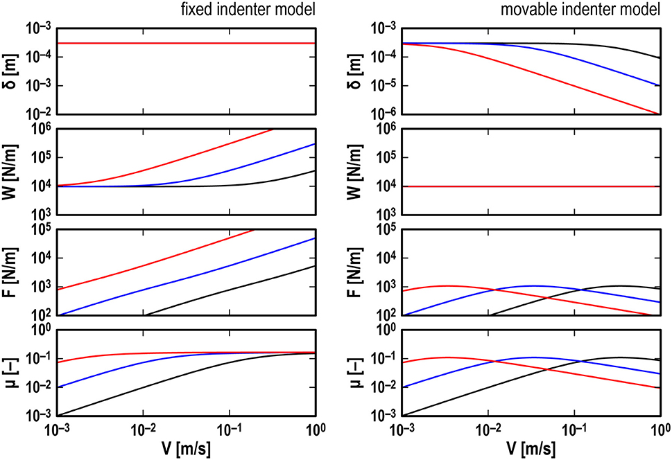
Figure 5. Numerical results in steady sliding for fixed indenter model (Left) and movable indenter model (Right): effects of retardation time τ on velocity dependences of indentation depth δ (Top), normal load W (second row), friction force F (third row), and friction coefficient μ (bottom row). Black lines, τ = 10⁻² s; blue lines, τ = 10⁻¹ s; red lines, τ = 10⁰ s (see Table 1 for other parameter values).

Through a series of numerical simulations under various sets of parameters, master curves on μ in the steady sliding for the two types of models were obtained (see Figure 6). The red curve in the left graph is the master curve for the FI model, the ordinate and abscissa of which are μ(R/δ)^1/2 and Vτ(Rδ)^−1/2, respectively, while the red curve in the right graph is the master curve for the MI model, the ordinate and abscissa of which are μ(KR²/W)^1/3 and Vτ(K/RW)^1/3, respectively. It should be stressed that every quantity assigned to the axes in Figure 6 is dimensionless.

FIGURE 6

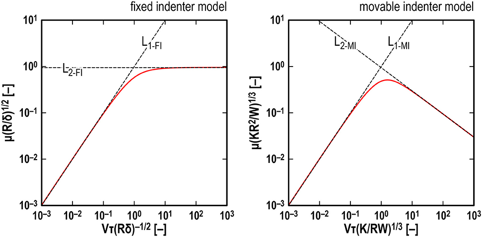
Figure 6. Master curves on friction coefficient μ in steady sliding for fixed indenter model (Left) and movable indenter model (Right). Red solid lines: master curves obtained numerically, black broken lines: asymptotes obtained theoretically.

To examine the asymptotes of the master curves, we again consider the two limiting cases:

$\begin{array}{ll}(x_{\text{LE}},x_{\text{TE}})=(-a,a)\text{ for }{l}_{\text{r}}\ll a(\text{steady sliding})& (38)\end{array}$

$\begin{array}{ll}(x_{\text{LE}},x_{\text{TE}})=(-a,0)\text{ for }{l}_{\text{r}}\gg a(\text{steady sliding})& (39)\end{array}$

where again, the former means the “non-peeling” of the entire contact area, and the latter means the “complete peeling” of the contact area in the outlet side. First, when l_r ≪ a, W and F can be estimated by

$\begin{array}{ll}W~{\displaystyle {\int }_{-a}^a}Ku(x)\text{d}x=2\alpha R^{1/2}K{\delta }^{3/2}& (40)\end{array}$

$\begin{array}{ll}F~{\displaystyle {\int }_{-a}^a}-h^{\prime }(x)C\stackrel{.}{u}(x)\text{d}x=2\alpha R^{-1/2}CV{\delta }^{3/2}& (41)\end{array}$

respectively, where $\alpha =2\sqrt{2}/3$. Therefore, μ for the first limiting case [Equation (38)] is given by

$\begin{array}{ll}\mu =\frac{CV}{RK}(\text{asymptotes }{\text{L}}_{\text{1-FI}}\text{ and }{\text{L}}_{\text{1-MI}})& (42)\end{array}$

Then, when l_r ≫ a, W and F can be estimated by

$\begin{array}{ll}W~{\displaystyle {\int }_{-a}^0}C\stackrel{.}{u}(x)\text{d}x=CV\delta & (43)\end{array}$

$\begin{array}{ll}F~{\displaystyle {\int }_{-a}^0}-h^{\prime }(x)C\stackrel{.}{u}(x)\text{d}x=\alpha R^{-1/2}CV{\delta }^{3/2}& (44)\end{array}$

respectively. Therefore, μ for the second limiting case [Equation (39)] is given by

$\begin{array}{ll}\mu =\alpha \sqrt{\frac{\delta }{R}}\left(\text{asymptote }{\text{L}}_{\text{2-FI}}\right)& (45)\end{array}$

or, by using Equation (43),

$\begin{array}{ll}\mu =\alpha \sqrt{\frac{W}{RCV}}\left(\text{asymptote }{\text{L}}_{\text{2-MI}}\right)& (46)\end{array}$

The black broken lines in Figure 6 are the above asymptotes. Now we find that excellent agreement of the asymptotes with the master curves. Note that Equations (42) and (46) are the same as those shown by Popov (2010).

Velocity Dependences of Friction Coefficient

In this section, based on Figure 6, let us consider the velocity dependences of the friction coefficient. In Figure 6, the drive velocity V is included only on the abscissa. Therefore, from the intersection of the two asymptotes, we introduce the critical velocity V^* defined as

$\begin{array}{ll}{V}^{*}~\frac{K\sqrt{R\delta }}{C}(\text{FI model})& (47)\end{array}$

$\begin{array}{ll}{V}^{*}~\frac{\sqrt[3]{R{K}^{2}W}}{C}(\text{MI model})& (48)\end{array}$

By using V^*, the formulas for estimating friction coefficient are summarized in Table 2.

TABLE 2

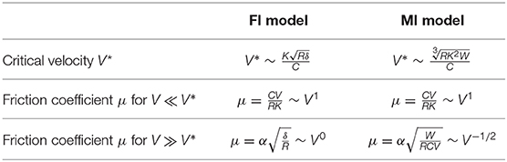
Table 2. Velocity dependences of friction coefficient in steady sliding ($\alpha =2\sqrt{2}/3$).

First, we consider the case of V ≪ V^*. From the third row of Table 2, we find that the formulas for both models are the same, which means that when V ≪ V^*, the vertical lift effect is negligible, although the rigid indenter could move vertically in the MI model. In addition, considering the assumption given by Equation (38), we find that when V ≪ V^*, the peeling of the contact area in the outlet side is also negligible in both models. The velocity dependence of μ is μ ~ V¹, which means that it is caused by the damping of the Kelvin–Voigt foundation.

Then, we consider the case of V ≫ V^*. From the bottom row of Table 2, we find that the formulas for the two types of models are different, which means that when V ≫ V^*, the vertical lift effect strongly appears in the MI model. From Equation (43), we find that the vertical lift effect appears according to

$\begin{array}{ll}\delta ~V^{-1}\text{ for }V\gg V^{*}(\text{MI model})& (49)\end{array}$

which is confirmed by the numerical results shown in the upper right graph of Figure 5, where a decrease in δ means an increase in z_A (= –δ): that is, the vertical lift of the rigid indenter. In addition, considering the assumption given by Equation (39), we find that when V ≫ V^*, the complete peeling of the contact area in the outlet side occurs in both models. Regarding the velocity dependence of μ in the FI model, it is μ ~ V⁰ (i.e., μ is constant). This is because when V ≫ V^*, the damping becomes dominant, and therefore the restoring becomes negligible, which leads to the situation that both of W and F are proportional to V, as shown in Equations (43) and (44). Regarding the velocity dependence of μ in the MI model, on the other hand, it shows the negative dependence μ ~ V^−1/2, which is caused by the vertical lift of the rigid indenter.

As a result, we find that in the MI model, the function μ = μ(V) has a local maximum at V ~V^*. Note that for many decades, this type of velocity dependence has been observed and discussed by a number of researchers for the sliding friction of elastomers, which seems to be basically understood as the frequency dependence of viscoelasticity (Persson, 2001; Momozono et al., 2010; Carbone and Putignano, 2013). However, the MI model produces a qualitatively similar dependence, although the frequency dependence of the Kelvin–Voigt foundation has no local maximum, where it is caused by the vertical lift of the rigid indenter.

Also note that the negative dependence μ ~ V^−1/2 means

$\begin{array}{ll}\mu \to 0\text{ for }\frac{V}{V^{*}}\to \infty (\text{MI model})& (50)\end{array}$

which gives us an idea of the ultra-low friction. If we try to embody the situation of Equation (50) in real systems, not only increasing V but also decreasing V^* is promising, the method of which is shown by Equation (48). Probably, the most effective parameter is the damping C (or the retardation time τ = C/K). According to the equation, increasing C leads to decreasing V^*, which leads to approaching the situation of Equation (50). It should be noted that the concept can never be embodied in the FI model, because increasing C under a constant δ just linearly increases F, as shown in Equation (44). Therefore, the key is the vertical lift effect arising with the movable boundary condition of the rigid indenter.

Recently, several swollen polymers showing ultra-low friction (e.g., hydrogels and polymer brushes) have attracted attention, with inspirations from natural tribosystems in human bodies (e.g., eyes and joints) (Klein et al., 1994; Lee and Spencer, 2008). An important aspect is obviously the low-adhesive properties of surfaces caused by their “microscopic” structures. However, as another important aspect, proper “macroscopic” structures are also needed to utilize them properly under various conditions. At least, recalling the results on the transient sliding (Figure 3), we can say that in the lubricated sliding of elastomers, macroscopic structures utilizing the vertical lift effect by viscoelasticity seem to have strong advantages for smooth transition to the fluid film lubrication regime, especially at the onset of sliding.

Conclusions

In this study, the sliding friction of elastomers was investigated numerically and theoretically for the line contact between a cylindrical rigid indenter and a “frictionless” Kelvin–Voigt foundation. The onset of sliding under an abrupt increase in the drive velocity was simulated with different boundary conditions of the rigid indenter. The main conclusions are as follows:

1. When the rigid indenter is not allowed to move in any direction, just an abrupt change in the friction force appears, which is not accompanied by any transient processes. However, when the rigid indenter is able to move in the vertical direction, the transient sliding friction including three different time constants appears, resembling the typical transition from the static friction to the kinetic friction, in spite of no static friction considered in the simulation. The aforementioned drastic difference is caused by the “vertical lift” of the rigid indenter induced by the damping of the Kelvin–Voigt foundation.

2. When the drive velocity is sufficiently low, the vertical lift effect is negligible, where the restoring is more dominant than the damping, which leads to little peeling of the entire contact area and the friction coefficient proportional to the drive velocity. On the other hand, when the drive velocity is sufficiently high, the vertical lift effect becomes strong, where the damping is more dominant than the restoring, leading to the complete peeling of the contact area in the outlet side. The vertical lift of the rigid indenter strongly affects the characteristics of the steady sliding friction, which is explained well by using the critical velocity determined from the asymptotes in the master curve of friction coefficient.

At the end, it is noted again that the foregoing conclusions are obtained for the Kelvin–Voigt foundation against a cylindrical rigid indenter. In general, since behaviors are greatly affected by the rheology of the viscoelastic foundation or the shape of the rigid indenter (Popov and Heß, 2015), further investigations are needed.

Data Availability Statement

All datasets generated for this study are included in the article/supplementary material.

Author Contributions

KN designed the study and wrote the manuscript. MK conducted the simulations. KN and MK analyzed the results. All authors contributed to the article and approved the submitted version.

Funding

This study was partly supported by ACCEL (Accelerated Innovation Research Initiative Turning Top Science and Ideas into High-Impact Values) under Grant No. JPMJAC1503 sponsored by Japan Science and Technology Agency.

Conflict of Interest

The authors declare that the research was conducted in the absence of any commercial or financial relationships that could be construed as a potential conflict of interest.

Acknowledgments

The authors gratefully acknowledge Professor Valentin L. Popov and Professor Hiroshi Watanabe for fruitful and stimulating discussions.

References

Barquins, M. (1985). Sliding friction of rubber and Schallamach waves: a review. Mater. Sci. Eng. 73, 45–63. doi: 10.1016/0025-5416(85)90295-2

CrossRef Full Text | Google Scholar

Belin, M., Arafune, H., Kamijo, T., Perret-Liaudet, J., Morinaga, T., Honma, S., et al. (2018). Low friction, lubricity, and durability of polymer brush coatings, characterized using the relaxation tribometer technique. Lubricants 6:52. doi: 10.3390/lubricants6020052

CrossRef Full Text | Google Scholar

Carbone, G., and Putignano, C. (2013). A novel methodology to predic tsliding and rolling friction of viscoelastic materials: theory and experiments. J. Mech. Phys. Solids 61, 1822–1834. doi: 10.1016/j.jmps.2013.03.005

CrossRef Full Text | Google Scholar

Fukahori, Y., and Yamazaki, H. (1994). Mechanism of rubber abrasion: part I: abrasion pattern formation in natural rubber vulcanizate. Wear 171, 195–202. doi: 10.1016/0043-1648(94)90362-X

CrossRef Full Text | Google Scholar

Gong, J. P., Kurokawa, T., Narita, T., Kagata, G., Osada, Y., Nishimura, G., et al. (2001). Synthesis of hydrogels with extremely low surface friction. J. Am. Chem. Soc. 123, 5582–5583. doi: 10.1021/ja003794q

PubMed Abstract | CrossRef Full Text | Google Scholar

Grosch, K. A. (1963). The relation between the friction and visco-elastic properties of rubber. Proc. Roy. Soc. Ser. A 274, 21–39. doi: 10.1098/rspa.1963.0112

CrossRef Full Text | Google Scholar

Johnson, K. L. (1985). Contact Mechanics. Cambridge: Cambridge University Press. doi: 10.1017/CBO9781139171731

CrossRef Full Text | Google Scholar

Klein, J., Kumacheva, E., Mahalu, D., Perahia, D., and Fetters, L. J. (1994). Reduction of frictional forces between solid surfaces bearing polymer brushes. Nature 370, 634–636. doi: 10.1038/370634a0

CrossRef Full Text | Google Scholar

Kusche, K. (2017). Frictional force between a rotationally symmetric indenter and a viscoelastic half-space. Z. Angew. Math. Mech. 97, 226–239. doi: 10.1002/zamm.201500169

CrossRef Full Text | Google Scholar

Lee, S., and Spencer, N. D. (2008). Sweet, hairy, soft, and slippery. Science 319, 575–576. doi: 10.1126/science.1153273

PubMed Abstract | CrossRef Full Text | Google Scholar

Li, Q., Dimaki, A., Popov, M., Psakhie, S. G., and Popov, V. L. (2015). Kinetics of the coefficient of friction of elastomers. Sci. Rep. 4:5795. doi: 10.1038/srep05795

PubMed Abstract | CrossRef Full Text | Google Scholar

Maegawa, S., and Nakano, K. (2010). Mechanism of stick-slip associated with Schallamach waves. Wear 268, 924–930. doi: 10.1016/j.wear.2009.12.018

CrossRef Full Text | Google Scholar

May, W. D., Morris, E. L., and Atack, D. (1959). Rolling friction of a hard cylinder over a viscoelastic material. J. Appl. Phys. 30, 1713–1724. doi: 10.1063/1.1735042

CrossRef Full Text | Google Scholar

Mizukami, M., Gen, M., Hsu, S. Y., Tsujii, Y., and Kurihara, K. (2019). Dynamics of lubricious, concentrated PMMA brush layers studied by surface forces and resonance shear measurements. Soft Matter. 15, 7765–7776. doi: 10.1039/C9SM01133A

PubMed Abstract | CrossRef Full Text | Google Scholar

Momozono, S., Nakayama, K., and Kyogoku, K. (2010). Theoretical model for adhesive friction between elastomers and rough solid surfaces. J. Chem. Phys. 132:114105. doi: 10.1063/1.3356220

PubMed Abstract | CrossRef Full Text | Google Scholar

Moore, D. F., and Geyer, W. A. (1972). A review of adhesion theories for elastomers. Wear 22, 113–141. doi: 10.1016/0043-1648(72)90271-2

CrossRef Full Text | Google Scholar

Moore, D. F., and Geyer, W. A. (1974). A review of hysteresis theories for elastomers. Wear 30, 1–34. doi: 10.1016/0043-1648(74)90055-6

CrossRef Full Text | Google Scholar

Nakano, K., Kawaguchi, K., Takeshima, K., Shiraishi, Y., Forsbach, F., Benad, J., et al. (2019). Investigation on dynamic response of rubber in frictional contact. Front. Mech. Eng. 5:9. doi: 10.3389/fmech.2019.00009

CrossRef Full Text | Google Scholar

Nakano, K., and Maegawa, S. (2009). Stick-slip in sliding systems with tangential contact compliance. Tribol. Int. 42, 1771–1780. doi: 10.1016/j.triboint.2009.04.039

CrossRef Full Text | Google Scholar

Nomura, A., Okayasu, K., Ohno, K., Fukuda, T., and Tsujii, Y. (2011). Lubrication mechanism of concentrated polymer brushes in solvents: effect of solvent quality and thereby swelling state. Macromolecules 44, 5013–5019. doi: 10.1021/ma200340d

CrossRef Full Text | Google Scholar

Persson, B. N. J. (2001). Theory of rubber friction and contact mechanics. J. Chem. Phys. 115, 3840–3861. doi: 10.1063/1.1388626

CrossRef Full Text | Google Scholar

Popov, V. L. (2010). Contact Mechanics and Friction: Physical Principles and Applications. Berlin: Springer. doi: 10.1007/978-3-642-10803-7

CrossRef Full Text | Google Scholar

Popov, V. L., and Heß, M. (2015). Method of Dimensionality Reduction in Contact Mechanics and Friction. Berlin: Springer. doi: 10.1007/978-3-642-53876-6

CrossRef Full Text | Google Scholar

Popov, V. L., Voll, L., Kusche, S., Li, Q., and Rozhkova, S. V. (2018). Generalized master curve procedure for elastomer friction takin into account dependencies on velocity, temperature and normal force. Tribol. Int. 120, 376–380. doi: 10.1016/j.triboint.2017.12.047

PubMed Abstract | CrossRef Full Text | Google Scholar

Rubinstein, S. M., Cohen, G., and Fineberg, J. (2004). Detachment fronts and the onset of dynamic friction. Nature 430, 1005–1009. doi: 10.1038/nature02830

PubMed Abstract | CrossRef Full Text | Google Scholar

Schallamach, A. (1957). Friction and abrasion of rubber. Wear 1, 384–417. doi: 10.1016/0043-1648(58)90113-3

CrossRef Full Text | Google Scholar

Schallamach, A. (1971). How does rubber slide? Wear 17, 301–312. doi: 10.1016/0043-1648(71)90033-0

CrossRef Full Text | Google Scholar

Tadokoro, T., Sato, K., Nagamine, T., Nakano, K., Sasaki, S., Sato, T., et al. (2020). Concentrated polymer brush as reciprocating seal material for low leakage and low friction. Tribol. Trans. 63, 20–27. doi: 10.1080/10402004.2019.1650213

CrossRef Full Text | Google Scholar

Williams, M. L., Landel, R. F., and Ferry, J. D. (1955). The temperature dependence of relaxation mechanisms in amorphous polymers and other glass-forming liquids. J. Am. Chem. Soc. 77, 3701–3707. doi: 10.1021/ja01619a008

CrossRef Full Text | Google Scholar

Yamaguchi, T., Morishita, M., Doi, M., Hori, T., Sakaguchi, H., and Ampuero, J. P. (2011). Gutenberg-Richter's law in sliding friction of gels. J. Geophys. Res. 116, B12306. doi: 10.1029/2011JB008415

CrossRef Full Text | Google Scholar