Passive Thermography Measurement of Damage Depth During Composites Load Testing

Introduction

The advantages of thermal nondestructive evaluation (NDE) are fast inspection times, large area coverage, and noncontact measurements. Therefore, thermography NDE is commonly used for composite inspection during mechanical loading. The earliest published works discussed the combination of thermal imaging with mechanical vibrations for the detection of damage in composites (Reifsnider and Williams, 1974; Henneke et al., 1979). This was an active thermography inspection where the mechanical loading was controlled and optimized to produce heating over areas of damage. This technique is also known as vibrothermograhy (Reifsnider et al., 1980). Over the years other techniques have been developed where mechanical vibrations were used to detect damage. A lock-in detection technique, where ultrasonic vibrations are synchronized with the IR camera's image acquisition, is used to increase sensitivity for damage detection (Busse et al., 1992; Rantala et al., 1996; Dillenz et al., 1999). In the early 2000s, the term sonic thermography was introduced (Favro et al., 2000). A sonic thermography technique was patented using infrared imaging and acoustic chaos sound energy to actively inspect a structure with mechanical vibrations (Favro et al., 2006) and recently a portable sonic thermography inspection system has been developed (Polimeno et al., 2014).

Unlike active thermography, passive thermography for composites testing does not require control of the mechanical vibrations or loading for the inspection. The infrared camera observes the surface temperature and also perhaps obtains load information. In other words, a mechanical load is applied but is not actively controlled for the purposes of inspection; the thermal camera is passively acquiring data. Passive thermography has been used extensively for composites inspection under both cyclic and quasistatic mechanical load. Various studies have been performed using passive thermography for damage detection in composites during cyclic fatigue (Toubal et al., 2006; Roche et al., 2013a,b; De Finis and Palumbo, 2020). Also, studies have been performed using passive thermography during quasistatic loading (Harizi et al., 2014; Crupi et al., 2015; Zalameda and Winfree, 2018). A major challenge for passive thermography during quasistatic loading, as compared to cyclic loading, is to detect the small nonrepetitive temperature changes. During composites testing, other techniques have been combined with passive thermography to improve damage detection. These techniques include acoustic emission and digital image correlation (Ringermacher et al., 2009; Kordatos et al., 2013; Crupi et al., 2015; Munoz et al., 2015; Zalameda et al., 2017). In addition, passive thermography has been used to determine fatigue limits on composites during load testing (La Rosa and Risitano, 2000; Montesano et al., 2012; Vergani and Colombo, 2014; Munoz et al., 2015). Most of these efforts mainly focused on coupon level testing, however, there have been studies performed using passive thermography on more complex structures such as composite cylinders and hat stiffened panels (Zalameda et al., 2012; Bisagni et al., 2014).

Recent work has shown that rapid growth damage formation during quasistatic loading of a single stringer panel produces heating that is composed of two heat generation components (Winfree et al., 2019). The first component is an instantaneous response due to an irreversible thermoelastic strain release due to rapid damage formation. The second component observed is mechanical heating due to fracture damage (separation of layers) that produces a heat flux at the interface of failure (Huanga et al., 2019). This produces a transient rise in surface temperature as a function of damage depth. The first component defines the thermal start time for the transient response. A one-dimensional thermal model is presented that takes into account both the instantaneous and fracture heating. This model is independent of the gap spacing between the delaminated layers. The one-dimensional thermal model was fitted to the data pixel by pixel, to produce imagery of the damage depth. The quasistatic thermal inspection results are compared to ultrasonic and X-ray CT data for damage size, shape and depth with relatively good agreement. It has been observed also, that during fatigue loading, similar rapid growth damage occurs. This rapid growth damage is challenging to detect during cyclic loading because the thermoelastic response is dominant. This paper discusses a data processing technique to detect and image the damage depth of the rapid growth damage for periodic or cyclic loading. Finally, these results show that passive thermography is able to detect the damage location, size, and depth during composites load testing. This will provide valuable information during load testing to precisely control the damage growth at various composite laminar interfaces and determine when the loading should be stopped to document the damage progression using ultrasonics or X-ray CT. The damage progression inspection database can then be used to validate test articles and damage progression models (Rose et al., 2013; Clay, 2017).

Experimental

Composite Samples Tested

The stiffened composite panel skin is 12 plies with a thickness of 0.22 cm, the stiffener flange is 12 plies thick with a thickness of 0.24 cm. The stiffener hat top is 16 plies with a thickness of 0.32 cm. The stiffener is a woven composite. Figures 1A–C show the stiffened composite panel stringer side, a painted specimen, and a cross sectional view, respectively. The overall panel dimensions are 25.4 × 25.4 cm. This panel is used for the quasistatic loading. The applied quasistatic loads are up to 1,000 pounds. The single stringer panel, used for fatigue loading, has the same geometry and thickness. Figures 1D,E show the stiffened composite panel skin side and stiffener side, respectively. The dimensions of the panel are width 21.6 cm and length 51.3 cm. The maximum applied cyclic fatigue loads are ~25,000 pounds for the single stringer panel. The frequency of the loading is 2 Hz.

FIGURE 1

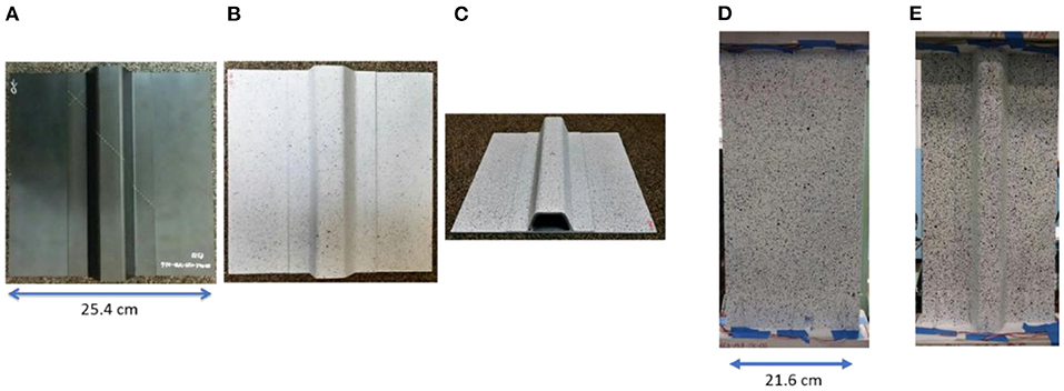
Figure 1. (A-E) composite single stringer hat stiffened panels used for quasistatic and fatigue loading.

Passive Thermography Systems for Quasistatic and Fatigue Loading

The test setups shown in Figures 2A,B are the quasistatic and fatigue loading configurations, respectively. The basic system consists of an IR camera operating in the 3–5 μm IR band and an image data acquisition computer. The IR camera is configured with 25 mm germanium optics. The focal plane array size of the camera is 640 × 512. The passive inspection captured the thermal variations during the loading. The setup required a Plexiglas^® shield to filter out spurious IR background sources (not shown in Figure 2). The camera frame rate is externally triggered and operated at up to 180 Hz. The load signal is also acquired using a USB based 12-bit data acquisition module. For each infrared camera frame, a load value is acquired. Furthermore, real time averaging, a delayed image subtraction, and real-time contrast adjustment are used to enhance detection of the small thermal transient signatures due to the damage (Zalameda and Winfree, 2018). The processed imagery is displayed in real time (~1 Hz) for the operator during testing. Without this processing, the faint thermal signatures that indicate damage would be difficult to detect in real time.

FIGURE 2

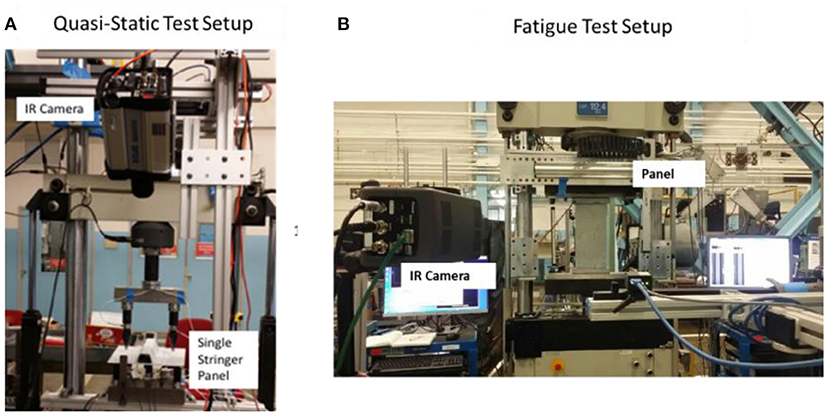
Figure 2. (A,B) passive thermography test setup used for quasistatic (left image) and fatigue loading (right image).

Measurement Results

Passive Thermography Results From Quasistatic Loading

Digital image processing is required to both enhance detection of thermal damage events and to facilitate comparison of the thermal inspection imagery to the ultrasonic or X-ray CT data. Typical parameters of 10 frames were boxcar averaged and a delay subtraction between the most recent averaged frame and the 100th averaged frame were used for real-time processing to produce the output image. The delayed subtraction removed fixed background infrared radiation while increasing sensitivity to changes. Additionally, for comparison to ultrasonic data, an image perspective transformation was used. The image perspective transformation was used to correct for the infrared camera view angle since the optical line of sight was not normal. The image correction is performed by defining four points mapped to a new set of four desired points (normal view) (Chan, 2012).

Figure 3 shows the instantaneous thermal response at 0.125 s. The thermally detected small delamination is similar in size and shape to the ultrasonic inspection. The thermal data were acquired at 80 Hz. Each averaged frame represented 0.125 s. The damage is semielliptical as confirmed by both the thermal and ultrasonic inspection images. The instantaneous heating component can be seen more clearly in Figure 4 where a single pixel is plotted over the damaged region center as a function of time. The instantaneous surface temperature increase occurs at ~79.8 s. Afterward, there is a significant transient increase in temperature occurring after 81.0 s. This heating is due to the fracture heating at the failure interface. This heat diffuses to the surface and the thermal time to reach maximum temperature is a function of damage depth and thermal diffusivity. Similarly, in Figure 5, the instantaneous thermal response for the large delamination failure is shown at 0.056 s. The thermally detected damage is similar in size and shape to the ultrasonic inspection. The thermal data were acquired at 180 Hz for the large delamination. Each averaged frame represented 0.056 s. The instantaneous heating component can be seen in Figure 6 where a single pixel is plotted over the damaged region center as a function of time. The instantaneous surface temperature increase occurs at ~41.7 s. Afterward, there is a dominant transient increase in temperature occurring after 43 s.

FIGURE 3

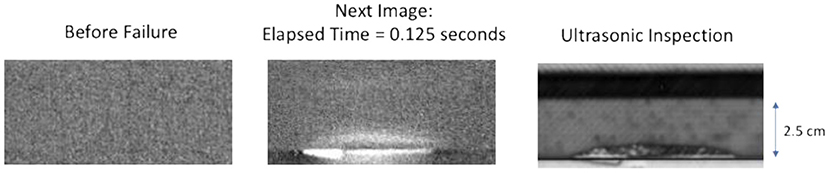
Figure 3. Comparison of instantaneous heating image to ultrasonic inspection for small delamination.

FIGURE 4

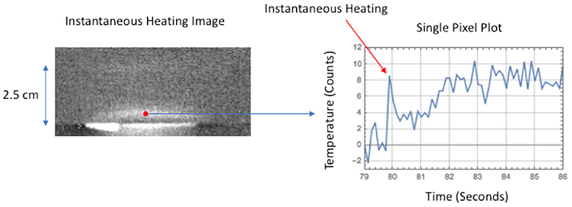
Figure 4. Single pixel plot of surface heating showing instantaneous heating response for small delamination.

FIGURE 5

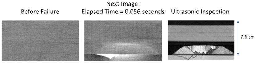
Figure 5. Comparison of instantaneous heating image to ultrasonic inspection for large delamination.

FIGURE 6

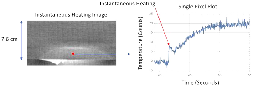
Figure 6. Single pixel plot of surface heating showing instantaneous heating response for large delamination.

Passive Thermography Results From Fatigue Loading

One area of interest is to capture the rapid temperature increase that results from damage events during fatigue loading. This can be masked by the significantly larger periodic temperature response due to the cyclic loading. The left images of Figure 7 display the thermoelastic response of the sample due to cyclic loading. These images are generated by averaging 10 frames and subtracting the averaged frames corresponding to the maximum and minimum temperature within a given cycle. For example, for 80 Hz acquisition frame rate and 10 frames averaged, there will be four average frames per cycle for a loading frequency of 2 Hz and two of those frames representing the maximum and minimum temperature will be subtracted. If the number of averages is adjusted to 40 frames, this will remove the periodic response. This can be viewed as a notch filter to remove the thermal response at 2 Hz in addition to any harmonic responses. The rapid growth thermal response is typically fracture damage at a given depth, which requires the heat to diffuse to the surface and will be typically much longer than the loading cycle time of 0.5 s. The most recent averaged frame is subtracted from the 30th averaged frame. The delay subtraction is sufficient to capture thermal transients that last 15 s or less. The notch filtered images with the delay subtraction, for the same data window, are shown in the right images of Figure 7. Using this processing, the periodic response at 2 Hz is removed thus revealing heating from sudden damage growth (indicated by the red arrows) and is not detectable in the periodic response left images. The periodic temperature response is plotted along with the filtered temperature response over the damage growth area (4 × 4 pixels average) in Figure 8. The periodic temperature response is removed to reveal the rapid growth damage temperature response. The instantaneous thermal heating is then used to determine the start time for the transient response. Using a thermal model, the depth of the damage can then be determined, and this is discussed in the next section.

FIGURE 7

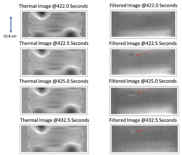
Figure 7. Single stringer composite panel analysis results showing periodic heating (left images) and rapid growth heating detection (right images).

FIGURE 8

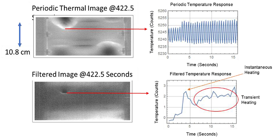
Figure 8. Single stringer composite panel with periodic and filtered temperature response.

One-Dimensional Modeling of Damage Heating

Series Solution for Instantaneous and Subsurface Heat Source

A one-dimensional solution was developed by Winfree et al. (2019) that models both the instantaneous and subsurface heating with perfect contact between layers and no convection losses. This model uses a series solution derived from the method of images and takes into account an instantaneous subsurface planar heat source buried between two layers (Carslaw and Jaeger, 1986). The analytic series solution is given as:

$\begin{array}{l}{T}_{planar}\left(t,l\right)\\ =\frac{Q}{K}\sqrt{\frac{\alpha }{\pi t}}\left(\text{ e}{}^{\frac{-l^2}{4\alpha t}}+{\displaystyle {\sum }_{N=1}^{\infty }(\text{e}{}^{\frac{-{\left(2LN-l\right)}^2}{4\alpha t}}+\text{ e}{}^{\frac{-{(2LN+l)}^2}{4\alpha t}})}\right)& (1)\end{array}$

where the buried source Q is the total energy per unit area, l is the depth of the source, t is time, K is thermal conductivity, α is the thermal diffusivity, and L is the total thickness of the layer. This time domain solution assumes there is no contact resistance at the buried heat source. The Laplace transform for a buried heat source at an interface with a contact resistance is given by

$\begin{array}{l}{T}_{planar}\left(s,l\right)\\ =\frac{\left(KR\sqrt{\frac{s}{\alpha }}+\coth (\left(L-l\right)\sqrt{\frac{s}{\alpha }})\right)Q}{K\sqrt{\frac{s}{\alpha }}\left(\cosh (l\sqrt{\frac{s}{\alpha }})+\sinh (l\sqrt{\frac{s}{\alpha }})(KR\sqrt{\frac{s}{\alpha }}+\coth \left(\left(L-l\right)\sqrt{\frac{s}{\alpha }}\right)) \right)}& (2)\end{array}$

where R is the contact resistance at the interface. The contact resistance R is equal to the air gap spacing divided by the thermal conductivity of air. Equation (2) is numerically inverted using the fixed Talbot algorithm (Talbot, 1979) to produce the time domain response. The thermal conductivity value used for air is 0.00026 W/cm/K. Other parameters used in Equation (2) were: Q is 1.0 Watt/cm², l is 0.22 cm, and L is 0.40 cm. The composite thermal conductivity was estimated to be K = 0.0045 W/cm/K (Colombo et al., 2011). The thermal diffusivity of the woven composite flange was measured previously using a two-sided thermal flash technique (Winfree and Heath, 1998). The thermal diffusivity value, α, measured was 0.0042 cm²/s. Equation (1) is equivalent to Equation (2) if the contact resistance is set to zero. Both equations are solved using the following parameters: Q = 1.0 Watt/cm², α = 0.0042 cm²/s, l = 0.1 cm, L = 0.2 cm, and K = 0.0045 W/cm/K. Equation (2) is numerically inverted using the fixed talbot algorithm (Chan, 2012) and this is equivalent to Equation (1) for infinite terms in the series. The number of terms to be used in the series solution of Equation (1) has to be determined to accurately simulate the one-dimensional heat flow. The root mean squared difference between Equation (2) and Equation (1) for series terms incremented from N = 1, 2, 3, 4, and 5 are 0.174, 0.00604, 0.00069, 2.395 × 10⁻⁷ and 2.42 × 10⁻¹⁰, respectively. The root mean squared difference error converges rapidly for N > 2 and therefore, N = 3 terms were sufficient to accurately simulate the one-dimensional heat flow for Equation (1). A comparison between the set of responses between Equations (1) and (2) are shown in Figure 9. The set of responses for Equation (2) is calculated for contact resistances representing air gap spacing distances of 0, 10, 20, and 40 μm. The Equation (2) responses are fits of the responses with Equation (1), where the parameters of the fit were l and Q. As can be seen from the figure, the data fits well with a maximum root mean square difference error of 0.041 for the 40 μm gap spacing. The values for the depth ranged from 0.22 (for no gap) to 0.20 (for 40 μm gap spacing) with an averaged error of 4.5%. Therefore, Equation (1) is adequate for estimation of the depth, since a more accurate estimation would require knowledge of the contact resistance or gap spacing. The instantaneous increase in surface temperature is assumed to be thermoelastic heating due to the change in curvature of the layer. The instantaneous thermoelastic energy density due to a change in curvature of a layer as a function of depth z, E(z), is given as:

$\begin{array}{ll}E(z)=E_0(1-2\frac{z}{L})\text{ where }{E}_o=-\frac{c\rho L}{2\sigma \Delta \varnothing }.& (3)\end{array}$

The variables of Equation (3) are: σ is the linear thermal expansion coefficient, ∅ is the change in radius of curvature, c is the heat capacity, ρ is the density, E₀ is the instantaneous thermoelastic energy density and L is again the total layer thickness. The change in radius of curvature is related to a change in strain thus providing the change in relative temperature. The instantaneous temperature response due to thermoelastic heating can then be found by convolving Equation (1) with Equation (3) and is given as:

$\begin{array}{ll}{T}_{TE}\left(t,l\right)={\displaystyle {\int }_0^l}{E}_0\left(1-\frac{2p}{L}\right)T_{planar}\left(t,p\right)dp& (4)\end{array}$

where p is the damage depth integration term. Solving for Equation (4) reveals the equation:

$\begin{array}{l}{T}_{TE}\left(t,l\right)=\frac{1}{Kl\sqrt{\pi }}{E}_{0}Q\sqrt{\frac{\alpha }{t}}(-4\alpha t+4\alpha e^{-\frac{49l^2}{4\alpha t}}t-8\alpha e^{-\frac{9l^2}{\alpha t}}t\\ +8\alpha e^{-\frac{25l^2}{4\alpha t}}t-8\alpha e^{-\frac{4l^2}{\alpha t}}t+8\alpha e^{-\frac{9l^2}{4\alpha t}}t-8\alpha e^{-\frac{l^2}{\alpha t}}t\\ +8\alpha e^{-\frac{l^2}{4\alpha t}}t+4\sqrt{\alpha }l\sqrt{\pi }\sqrt{t}\text{Erf}[\frac{l}{2\sqrt{\alpha }\sqrt{t}}]\\ -8\sqrt{\alpha }l\sqrt{\pi }\sqrt{t}\text{Erf}[\frac{l}{\sqrt{\alpha }\sqrt{t}}]+12\sqrt{\alpha }l\sqrt{\pi }\sqrt{t}\text{Erf}\\ \left[\frac{3l}{2\sqrt{\alpha }\sqrt{t}}\right]-16\sqrt{\alpha }l\sqrt{\pi }\sqrt{t}\text{Erf}\left[\frac{2l}{\sqrt{\alpha }\sqrt{t}}\right]\\ +20\sqrt{\alpha }l\sqrt{\pi }\sqrt{t}\text{Erf}\left[\frac{5l}{2\sqrt{\alpha }\sqrt{t}}\right]-24\sqrt{\alpha }l\sqrt{\pi }\sqrt{t}\text{Erf}\\ \left[\frac{3l}{\sqrt{\alpha }\sqrt{t}}\right]+13\sqrt{\alpha }l\sqrt{\pi }\sqrt{t}\text{Erf}[\frac{7l}{2\sqrt{\alpha }\sqrt{t}}]).& (5)\end{array}$

The total surface temperature response can then be given as the linear combination of the instantaneous thermoelastic heating, Equation (5) with the subsurface heating given in Equation (1). This is given as:

$\begin{array}{ll}{T}_{total}\left(t,l\right)=T_{TE}\left(t,l\right)+T_{planar}\left(t,l\right)& (6)\end{array}$

where again l is the depth of damage. The temperature response equation assumes no convection losses and the heat flux generated is considered instantaneous. For a known thermal diffusivity, Equation (6) can be used to determine the damage depth, pixel by pixel, by minimizing the squared difference between the model and measured response using a three parameter fit of damage depth l, the instantaneous thermoelastic energy density E₀, and the equilibrium temperature term Q α /K. Equation (6) is plotted in Figure 10 for l varied at damage depths of 0.20, 0.25, and 0.30 cm and with E₀ = 1.0 Watt/cm² and the overall thickness L = 0.40 cm. For Equation (6), as expected for the early times, the temperature response is dominated by the instantaneous thermal heating. For the later times the thermal response is dominated by the transient heating. As shown in Figure 10, Equation (6) predicts if the damage is deeper, the temperature will take more time to come to an equilibrium value as expected.

FIGURE 9

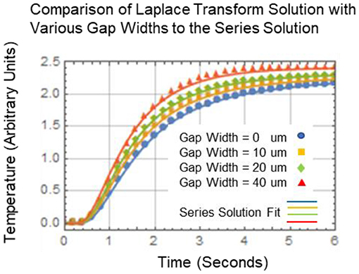
Figure 9. Comparison between the series solution of Equation (1) and the numerically inverted results of Equation (2) for various air gap spacing.

FIGURE 10

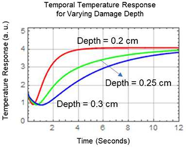
Figure 10. Temporal temperature plots of Equation (6) showing thermal response variation for varying damage depths.

Measurement Results

Quasistatic Load Damage Depth Imaging

Equation (6) was used to reduce the thermal data into a depth map image by fitting the thermal data pixel by pixel by minimizing the squared difference between the model and measured response using a three parameter fit of damage depth l, the instantaneous thermoelastic energy density E₀, and the equilibrium temperature term Q α /K. The thermal diffusivity was measured previously and the value used for the model fit was 0.0042 cm²/s. Example model fits to the thermal data, for a single pixel point (located approximately in the damage center) for the both the small and large delaminations, are displayed in Figure 11.

FIGURE 11

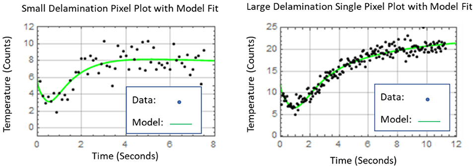
Figure 11. Examples of model curve fit to data for both small delamination and large delamination.

The thermally determined depth map images, obtained from the curve fitting for both the small delamination and large delamination, are displayed in Figure 12. A comparison between the ultrasonic and thermal measurement of the delamination size is shown in Table 1. The percent difference between thermal results, as compared to the ultrasonic measurements of damage length and width, was on average 15%. For the large delamination, the size and shape compares relatively well between the ultrasonic and thermal measurements. The large delamination maximum length and width for the ultrasonic measurements are length = 10.7 cm and width = 1.7 cm and the maximum length and width for the thermal measurements are length = 10.9 cm and width = 1.9 cm. The thermal measurements are slightly larger most likely due to in-plane heat flow. For the small delamination, the size and shape did not compare well between the ultrasonic and thermal measurements with an averaged percent difference of 23.6%. The small delamination maximum length and width for the ultrasonic measurements are length = 7.1 cm and width = 0.7 cm and the maximum length and width for the thermal measurements are length = 6.3 cm and width = 1.0 cm. The thermal length measurement is smaller as compared to the ultrasonic measurements. A possible reason for this is the small delamination fracture did not produce a significant amount of thermal energy that could be detected by the infrared camera. This can be seen in the instantaneous thermal image shown in Figure 3 where the thermal signature is not as pronounced on the right side of the delamination. This could be due to the change in curvature and heating during fracture was not significant enough to produce detectable heating. The maximum width of the thermal measurement was larger than the ultrasonic measurement and this again is most likely due to in-plane heat flow.

FIGURE 12

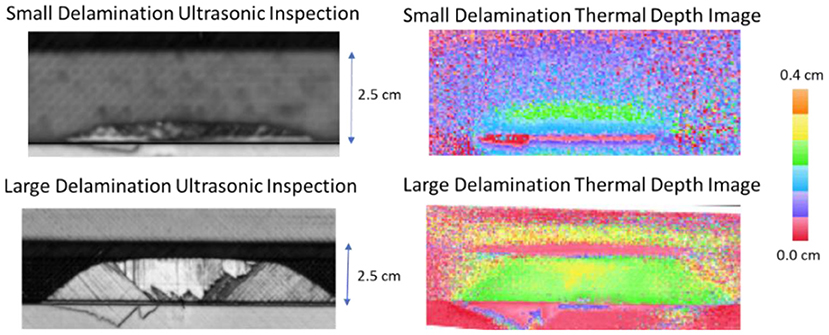
Figure 12. Comparison of curve fit depth map imaging to ultrasonic inspections for both small delamination and large delamination.

TABLE 1

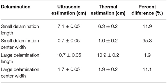
Table 1. Comparison of thermal to ultrasound measurement of delamination.

Shown in Figures 13, 14 are the respective line plots and X-ray CT cross-section imagery for both the small delamination and large delamination. A comparison between the X-ray CT and thermally measured crack depths are summarized in Table 2. For the small delamination, the crack depth is measured ~0.1 cm from the edge of the stiffener flange toward the hat at three different points A, B, and C, which are defined as left (1.2 cm from center), center, and right (1.2 cm from center), respectively. The X-ray CT imagery represents a subsection of the crack and not the full length due to field of view and resolution trade-offs. The X-ray CT measured depth for points A, B, and C appears to vary between 0.20 and 0.25 cm over the damaged area. This is confirmed from the thermal measurement results for points A, B, and C, which shows the crack depth varying between 0.20 and 0.23 cm at these three points. Also note the thermally measured depth away from the damage gives erroneous values due to the lack of a thermal response. For the large delamination, the crack depth is measured ~1 cm from the edge of the stiffener flange toward the hat at three different points A, B, and C, which are defined as left (2.5 cm from center), center, and right (2.5 cm from center), respectively. The X-ray CT imagery represents a subsection of the crack and not the full length due to field of view and resolution trade-offs. The X-ray CT measured depth for points A, B, and C, appears to vary between 0.24 and 0.29 cm over the damaged area. This is confirmed from the thermal measurement results for points A, B, and C which shows the crack depth varying between 0.24 and 0.30 cm at these three points. From the X-ray CT image it is clearly seen that the damage depth is deeper in the center (point B) and the depth slightly decreases away from the center. Also the X-ray CT clearly shows some cracks at multiple interfaces which cannot be detected using this thermal technique. This is a limitation since the thermal model accounts for one planar heat flux source. For both the small and large delamination, the percent difference between the thermal results, as compared to the X-ray CT measurements for damage depth was on average 7%. This difference error appears typical especially since the thermal model did not take into account the gap spacing which is unknown during load testing.

FIGURE 13

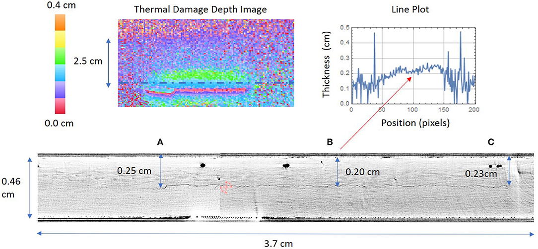
Figure 13. Thermal damage depth image and line plot for small delamination with comparison to X-ray CT cross section slice. At three different locations (A–C).

FIGURE 14

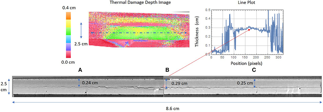
Figure 14. Thermal damage depth image and line plot for large delamination with comparison to X-ray CT cross section slice. At three different locations (A–C).

TABLE 2

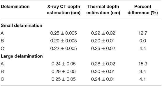
Table 2. Comparison of thermal to X-ray CT for damage depth.

Periodic Load Damage Depth Imaging

The thermal response due to periodic loading is dominated by thermoelastic heating. Applying the notch filter, as discussed in section Passive Thermography Results from Fatigue Loading, removes the periodic thermoelastic heating and reveals the heating due to rapid growth damage. The rapid growth damage contains the instantaneous and transient thermal responses. Shown in Figure 15 is an example model fit of Equation (6) to the thermal data for an area of 4 × 4 pixel points (located by the arrow in Figure 15) over the delamination. Again, by fitting the thermal model to the data, pixel by pixel, the thermal data can be reduced to a depth map image revealing the damage depth. This is shown in Figure 16. The thermally measured depth image reveals damage at depths around 0.19 cm. The thermal data were obtained during load testing and the loading was not stopped for ultrasound or X-ray CT characterization and therefore, no comparisons can be made for validation. Unlike the static loading measurements, the thermal data were acquired with the camera facing the panel's skin side. The skin thickness is ~0.22 cm thick. The damage depth of 0.19 cm would indicate the rapid growth damage would be near the skin stringer interface.

FIGURE 15

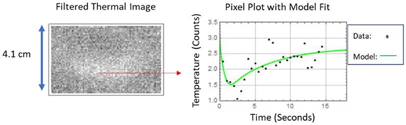
Figure 15. Example model fit to the filtered thermal data.

FIGURE 16

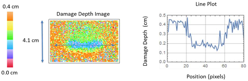
Figure 16. Model fit damage depth image with line plot showing damage depth values.

Conclusions

Passive thermography has been shown to be an effective real time NDE inspection technique to detect rapid growth (severe degradation) damage in a composite single stringer test panel during both quasistatic and cyclic loading. The size, shape, location, and depth of the damage can be detected. A one-dimensional thermal model, that is independent of delamination damage gap spacing, is presented and fitted to the data pixel by pixel, to produce imagery of the damage size and depth. The percent difference between thermal results, as compared to the ultrasonic measurements of damage length and width, was on average 15%.

A limitation of this technique is the potentially low signal to noise of the thermal signatures. For example, large errors were obtained for the small delamination length and width measurements (average of 23.6%). This is likely due to both the instantaneous and transient heating were small as compared to the large delamination. This is confirmed by the X-ray CT data which shows a much larger fracture as compared to the small delamination. The percent difference between the thermal results, as compared to the X-ray CT measurements for damage depth was on average 7%. This percent difference error is expected since the model did not take into account the gap spacing. The application of the notch filter allows for the measurement of rapid growth damage size and depth during cyclic loading. Of particular interest during composites testing is determining when the damage has transitioned to another interface. Future work could involve rapidly determining the depth of the damage as it appears during loading. This would require a more sophisticated processing technique. One approach is to use a denoising algorithm along with the use of Parkers method (Parker et al., 1961) for rapid determination of damage depth. This could be potentially helpful to structural test engineers by providing real time NDE of damage depth during composites load testing.

Data Availability Statement

The datasets presented in this article are not readily available because if the data is requested for release it will need to be approved through the NASA Langley approval process. Requests to access the datasets should be directed to; joseph.n.zalameda@nasa.gov.

Author Contributions

All authors listed have made a substantial, direct and intellectual contribution to the work, and approved it for publication.

Funding

This research was performed under NASA's Advanced Composite Project.

Conflict of Interest

The authors declare that the research was conducted in the absence of any commercial or financial relationships that could be construed as a potential conflict of interest.

Acknowledgments

The authors would like to thank composite testing leads Cheryl A. Rose and Wade C. Jackson of NASA Langley for composite sample preparation and load testing.

References

Bisagni, C., Davila, C. G., Rose, C., and Zalameda, J. N. (2014). “Experimental evaluation of damage progression in postbuckled single stiffener composite specimens,” in American Society for Composites 29th Technical Conference Proceedings, US-Japan 16, ASTM D30 (Seattle, WA).

Google Scholar

Busse, G., Bauer, M., Rippel, W., and Wu, D. (1992). “Lockin vibrothermal inspection of polymer composites,” in Quantitative Infrared Thermography, QIRT 92, Hrsg. Balageas, D., Busse, G., and Carlomagno, G. M., (Paris: Editions Européennes Thermique et Industrie), 154–159. doi: 10.21611/qirt.1992.024

CrossRef Full Text | Google Scholar

Carslaw, H. S., and Jaeger, J. C. (1986). Conduction of Heat in Solids, 2nd Edn. Oxford: Clarendon Press, 297–326.

Google Scholar

Chan, M. (2012). Perspective Control/Correction. Available online at: https://www.mathworks.com/matlabcentral/fileexchange/35531-perspective-control–correction (accessed January 10, 2018).

Clay, S. (2017). How ready are progressive damage analysis tools? Compos. World 3, 8–10. Available online at: https://www.compositesworld.com/articles/how-ready-are-progressive-damage-analysis-tools

Colombo, C., Libonati, F., Pezzani, F., Salerno, A., and Vergani, L. (2011). Fatigue behavior of a GFRP laminate by thermographic measurements. Proc. Eng. 10, 3518–3527. doi: 10.1016/j.proeng.2011.04.579

CrossRef Full Text | Google Scholar

Crupi, V., Guglielmino, E., Risitano, G., Risitano, F., and Tavilla, F. (2015). Experimental analyses of SFRP material under static and fatigue loading by means of thermographic and DIC techniques. Composit. Part B Eng. 77, 268–277. doi: 10.1016/j.compositesb.2015.03.052

CrossRef Full Text | Google Scholar

De Finis, R., and Palumbo, D. (2020). Estimation of the dissipative heat sources related to the total energy input of a CFRP composite by using the second amplitude harmonic of the thermal signal. Materials 13:2820. doi: 10.3390/ma13122820

PubMed Abstract | CrossRef Full Text | Google Scholar

Dillenz, A., Busse, G., and Wu, D. (1999). “Ultrasound lock-in thermography: feasibilities and limitations,” in Proceedings SPIE 3827, Diagnostic Imaging Technologies and Industrial Applications (Munich). doi: 10.1117/12.361008

CrossRef Full Text | Google Scholar

Favro, L. D., Han, X., Ouyang, Z., Sun, G., Sui, H., and Thomas, R. L. (2000). Infrared imaging of defects heated by a sonic pulse, Rev. Sci. Inst. 71, 2418–2421. doi: 10.1063/1.1150630

CrossRef Full Text | Google Scholar

Favro, L. D., Thomas, R. L., Han, X., Rothenfusser, M. J., Baumann, J. B., Shannon, R. E., et al. (2006). System and Method for Aacoustic Chaos and Sonic Infrared Imaging. U.S. Patent No. 7,516,663 B2. Washington, DC: U.S. Patent and Trademark Office.

Google Scholar

Harizi, W., Chaki, S., Bourse, G., and Ourak, M. (2014). Mechanical damage assessment of glass fiber-reinforced polymer composites using passive infrared thermography. Compos. Part B Eng. 59, 74–79. doi: 10.1016/j.compositesb.2013.11.021

CrossRef Full Text | Google Scholar

Henneke, E. G., Reifsnider, K. L., and Stinchcomb, W. W. (1979). Thermography—an NDI method for damage detection. JOM 31, 11–15. doi: 10.1007/BF03354475

CrossRef Full Text | Google Scholar

Huanga, B., Pastor, M. L., Garnier, C., and Gonga, X. J. (2019). A new model for fatigue life prediction based on infrared thermography and degradation process for CFRP composite laminates. Int. J. Fatigue 120, 87–95. doi: 10.1016/j.ijfatigue.2018.11.002

CrossRef Full Text | Google Scholar

Kordatos, E., Dassios, K. G„ Aggelis, D. G., and Matikas, T. E. (2013). Rapid evaluation of the fatigue limit in composites using infrared lock-in thermography and acoustic emission. Mech. Res. Commun. 54, 14–20, doi: 10.1016/j.mechrescom.2013.09.005

CrossRef Full Text | Google Scholar

La Rosa, G., and Risitano, A. (2000). Thermographic methodology for rapid determination of the fatigue limit of materials and mechanical components. Int. J. Fatigue 22, 65–73. doi: 10.1016/S0142-1123(99)00088-2

CrossRef Full Text | Google Scholar

Montesano, J., Bougherara, H., and Fawaz, Z. (2012). “Using infrared thermography for assessing the fatigue behavior of polymer matrix composites,” in ECCM15-15th European Conference on Composite Materials (Venice)24–28.

Google Scholar

Munoz, V., Vales, B., Perrin, M., Pastor, M. L., Welemane, H., Cantarel, A., et al. (2015). Damage detection in CFRP by coupling acoustic emission and infrared thermography. Compos. Part B Eng. 85, 68–75, doi: 10.1016/j.compositesb,.2015.09.011

CrossRef Full Text | Google Scholar

Parker, W. J., Jenkins, R. J., Butler, C. P., and Abbott, G. (1961). Flash Method of determining thermal diffusivity, heat capacity, and thermal conductivity. J. Appl. Phys, 32, 1679–1684. doi: 10.1063/1.1728417

CrossRef Full Text | Google Scholar

Polimeno, U., Almond, D. P., Weekes, E. W., and Chen, J. (2014). A compact thermosonic inspection system for the inspection of composites. Compos. Part B Eng. 59, 67–73. doi: 10.1016/j.compositesb.2013.11.019

CrossRef Full Text | Google Scholar

Rantala, J., Wu, D., and Busse, G. (1996). Amplitude modulated lock-in vibrothermography for NDE of polymers and composites. Res. Nondestruct. Eval. 7, 215–228. doi: 10.1080/09349849609409580

CrossRef Full Text | Google Scholar

Reifsnider, K. L., Henneke, E. G., and Stinchcomb, W. W. (1980). “The mechanics of vibrothermography,” in Mechanics of Nondestructive Testing, eds Stinchcomb, W. W., Duke, J. C., Henneke, E. G., and Reifsnider, K. L., (Boston, MA: Springer), 249–276. doi: 10.1007/978-1-4684-3857-4_12

CrossRef Full Text | Google Scholar

Reifsnider, K. L., and Williams, R. S. (1974). Determination of fatigue-related heat emission in composite materials. Exp. Mech. 14:479. doi: 10.1007/BF02323148

CrossRef Full Text | Google Scholar

Ringermacher, H. I., Howard, D. R., Knight, B. E., Plotnikov, Y. A., Osterlitz, M. J., Li, J., et al. (2009). System and Method for Locating Failure Events in Samples Under Load. U.S. Patent No. US6998616B2. Washington DC: U.S. Patent and Trademark Office.

Google Scholar

Roche, J.-M., Balageas, D., Lamboul, B., Bai, G., Passilly, F., Mavel, A., et al. (2013a). “Passive and active thermography for in situ damage monitoring in woven composites during mechanical testing,” in The 39th Annual Review of Progress in Quantitative Nondestructive Evaluation, AIP Conference Proceedings 1511, 555–562. doi: 10.1063/1.4789096

CrossRef Full Text | Google Scholar

Roche, J.-M., Balageas, D., Lapeyronnie, B., Passilly, F., and Mavel, A. (2013b). “Use of infrared thermography for in situ damage monitoring in woven composites,” in Photomechanics Conference; 27–29 May 2013 (Montpellier).

Google Scholar

Rose, C. A., Dávila, C. G., and Leone, F. A. (2013). Analysis Methods for Progressive Damage of Composite Structures; NASA/TM-2013-218024. Hampton, VA: NASA Langley Research Center.

Google Scholar

Talbot, A. (1979). The accurate numerical inversion of laplace transforms. IMA J. Appl. Math. 23, 97–120. doi: 10.1093/imamat/23.1.97

CrossRef Full Text | Google Scholar

Toubal, L., Karama, M., and Toubal, L. (2006). Damage evolution and infrared thermography in woven composite laminates under fatigue loading. Int. J. Fatigue 28, 1867–1872. doi: 10.1016/j.ijfatigue.2006.01.013

CrossRef Full Text | Google Scholar

Vergani, L., Colombo, C, and Libonati, F. (2014). A review of thermographic techniques for damage investigation in composites. Frattura ed Integrità Strutturale 27, 1–12. doi: 10.3221/IGF-ESIS.27.01

CrossRef Full Text | Google Scholar

Winfree, W. P., and Heath, D. M. (1998). “Thermal diffusivity imaging of aerospace materials and structures,” in Proceedings of SPIE, Thermosense XXIII, Vol. 3361 (Orlando, FL), 282–290. doi: 10.1117/12.304739

CrossRef Full Text | Google Scholar

Winfree, W. P., Zalameda, J. N., and Horne, M. R. (2019). Simulations of thermal signatures of damage measured during quasistatic loading of a single-stringer panel. AIP Conf. Proc. 2102:120007. doi: 10.1063/1.5099849

CrossRef Full Text | Google Scholar

Zalameda, J., and Winfree, W. (2018). Detection and characterization of damage in quasistatic loaded composite structures using passive thermography. Sensors 18:3562. doi: 10.3390/s18103562

CrossRef Full Text | Google Scholar

Zalameda, J. N., Burke, E. R., Horne, M. R., and Madaras, E. I. (2017). “Large area nondestructive evaluation of a fatigue loaded composite structure,” in Residual Stress, Thermomechanics and Infrared Imaging, Hybrid Techniques and Inverse Problems, Vol. 9, Proceedings of the 2016 Annual Conference on Experimental and Applied Mechanics, eds Quinn, S., and Balandraud, X., ISBN 978-319-42254-1, Chapter 4, doi: 10.1007/978-3-319-42255-8_4

CrossRef Full Text | Google Scholar

Zalameda, J. N., Burke, E. R., Parker, R. F., Seebo, J. P., Wright, C. W., and Bly, J. B. (2012). “Thermography inspection for early detection of composite damage in structures during fatigue loading,” in Thermosense XXXIV, Proceedings of SPIE Vol. 835403 (Baltimore, MD). doi: 10.1117/12.918127

CrossRef Full Text | Google Scholar