Localized Defect Detection from Spatially Mapped, In-Situ Process Data With Machine Learning

Introduction

Additive manufacturing (AM) is a set of exciting and promising processing methods that are expected to continue to revolutionize manufacturing. One exciting subset is AM for metals, which is being investigated for applications in several industries such as aerospace, automotive, biomedical, and nuclear (Herderick, 20112011), (Lou and Gandy, 2019) The excitement behind AM is attributed to its flexibility in component design—AM may be used to fabricate geometries not possible by other conventional means.

At the same time, however, the technologies have not achieved widespread adoption and are typically relegated to non-critical applications. The inability to gain traction comes from the poor repeatability of the process from one build to the next stemming from the prevalence of seemingly stochastic defects (Grasso and Colosimo, 2017) and anisotropic microstructure (Kok et al., 2018) yielding inconsistent and heterogeneous properties throughout a component and across nominal duplicates of a component. This is true for all metal AM technologies including the more mature subdomain of powder bed fusion (PBF).

The key to mitigating these shortcomings is to characterize more accurately the complex relationships between the PBF processes, the components’ structural characteristics (both microstructural as well as macro-scale defects), and the resulting mechanical properties that ultimately dictate the quality of the component. These sets of intricately coupled relationships have collectively been deemed process-structure-property relationships (DebRoy et al., 2018).

Some researchers have proposed the use of machine learning (ML) as a way to establish relationships between these different regimes. Such relationships would aid in more robust qualification of AM builds. The ultimate goal would be to predict component characteristics and mechanical properties from in-situ process data collected during fabrication. This would allow for circumvention of costly ex-situ characterization and destructive testing. Additionally, discovering and leveraging relationships between in-situ process data and component properties would allow for the determination of part properties in real-time during fabrication and possibly even the triggering of reparative measures.

Currently, research predominantly focuses on some form of in-situ imaging data for localized defect detection and property prediction as well as closed-loop control (Everton et al., 2016) (Moltumyr et al., 2020). However, other, less utilized in-situ data—specifically temporal sensor data—is also being investigated for process quality monitoring. Several commercial machines yield such data in the form of a build log file. Much of the data in build log files is generated by sensors that directly monitor machine subsystems and the build environment, the status of which can directly affect build quality (Sames et al., 2016). Analyzing these streams may help to directly relate the process to corresponding properties.

Recent work has shown the value of this temporal sensor data for build qualification—especially for electron beam PBF (EB-PBF). Grasso et al. (Grasso et al., 2018) showed how a statistical model could leverage data from Arcam log files to predict swelling. Additionally, Chandrasekar et al. (2019) showed how rake data from these log files, in addition to powder reuse information, informs build quality. Steed et al. (Steed et al., 2017) shows how a visual analysis tool called Falcon may be used for EB-PBF builds to analyze the time series data from log files to determine process consistency and relate it to build quality. Currently, however, it has been only possible to use these data on a layer-wise or build-wise basis; no published technique exists to leverage this data for more localized, intra-layer analyses.

Some machines produce sensor data records at a sufficient sampling rate to detect changes in these important subsystems during a single layer and even during a single melt-phase. However, leveraging this data for localized analysis is unintuitive due to its different modality—temporal instead of spatial. As such, some technique must be used to convert the temporal data to space in order to have a one-to-one relationship with the spatial data. Vandone et al. (Vandone et al., 2018) have proposed leveraging tool paths for directed energy deposition (DED) to fuse spatial (melt track morphology data) and temporal (melt pool imaging video data and laser power) datasets together for modeling. However, their work centers on experimental data from single melt tracks, the temporal input feature space is small and targeted, and the overall findings are likely not to scale to larger and more complex geometries and will be confounded by other process intricacies. Our approach, rather than being bottom up, begins to chip away at the process monitoring and defect detection problem in a top-down way. We begin with data from multiple full-scale builds and fuse together as many in-situ process signals as are available and leverage ML to mine for relationships between the process and structure.

For this study, we focus on a ConceptLaser M2 Laser Powder Bed Fusion (L-PBF) machine instead of Arcam EBM or DED sensor data. It records data from multiple sensors during a build and compiles it into a log file. Several of these data streams contain enough records to allow for investigating how perturbations in these process signals relate to localized defects that are detectable in in-situ layer-wise images. This work demonstrates an initial attempt of leveraging these temporal process data to detect localized, layer-wise defects within four entire builds using XGBoost. Additionally, we analyze the XGBoost prediction results to better understand key relationships between process data and the resulting defects.

This work specifically investigates the relationship between the process data and the occurrence of soot within a layer. Soot has been shown to cause significant degradation within the L-PBF process. While studying the effects of powder reused in L-PBF processes, Heiden et al. (Heiden et al., 2019) found that soot is potentially detrimental to both mechanical properties of components and to the reuse of powders for subsequent builds. They recommend process parameter tuning to reduce the occurrence of soot and spatter. Huang and Li (Huang and Li, 2021) found that the prevalence of soot that has resettled is likely related to decreased ductility of components due to reduced effective laser power in those regions. Finally, in a recent white paper GE additive discusses the poor materials processing that occurs as a result of soot and outlines ways that they are improving the gas flow systems on the ConceptLaser M2 machines to remove soot from the build area more effectively (Roidl).

Materials and Methods

Data Sources and Descriptions

This work was performed on process data produced from four builds fabricated at the Oak Ridge National Laboratory’s (ORNL) Manufacturing Demonstration Facility. Here we outline relevant information about the builds and the data collection procedure.

Build Setups and Descriptions

The builds were fabricated on a ConceptLaser M2 L-PBF system that has two 400 W laser modules and a build chamber volume of 245 mm × 245 mm x 450 mm. Four builds were chosen that had approximately the same geometry to reduce confounding effects that different geometries induce in the in-situ process data—especially the trajectory laser data. Figure 1 shows the two geometries included in this analysis.

FIGURE 1

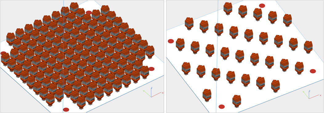
FIGURE 1. Left: geometry for build 1. Right: geometry for builds 2, 3, and 4. For builds 1 and 2 the gray and red regions represent where laser modules 1 and 2 are used respectively.

The builds were fabricated out of 316L stainless steel. Power was set to 370 W, speed to 1,350 mm/s, spot size to 130 μm, and hatch spacing to 0.09 mm. The gas flow rate was set at 52 mm/h, and the powder dosing factor was set to 350%. Builds 1 and 2 utilize both laser modules for different sections of the build. Build 3 uses only laser module 1; build 4 utilizes only laser module 2. Note that these builds were not fabricated specifically for this analysis. Instead, this work demonstrates the training, prediction, and analysis of an ML model on real-world data.

Data Collection and Description

Data were collected during the fabrication of these builds from several different distinct sources. These data sources are in-situ process data from various machine sensors that are recorded in log files, trajectory data that record relevant information about the laser scan path for each layer, and finally defect detection labels that were derived from in-situ visible-light layer-wise images.

In situ Process Data

During builds, the ConceptLaser M2 machine records data from several different in-situ sensors that monitor important subsystem statuses. These sensors monitor the build environment during fabrication and perturbations in these sensor signals may correlate with the quality of the fabricated component. In L-PBF the build chamber is filled with an inert gas, typically argon, to prevent oxidation of the material during fabrication. The laminar gas flow serves to mitigate the occlusion of the melt surface caused by the laser scattering off of the vapor plume and to remove spatter, soot, and other ejecta from the build area. A number of embedded sensors monitor this gas flow and the system that controls it.

In addition to gas flow rate, the machine monitors the oxygen concentration within the machine. The L-PBF process must be conducted within an inert environment because oxygen can react with the material during fabrication and lead to variable consistency and properties. Several sensors detect the level of residual oxygen in the system.

Finally, thermocouples are also placed in several location in the build chamber to monitor the global temperature. Figure 2 shows an example plot of temporal, in-situ process data from a gas flow sensor for one layer.

FIGURE 2

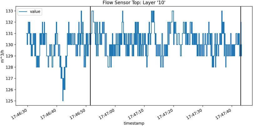
FIGURE 2. A plot of a single layer of log file data for “FlowSensorTop” from build 1. The black vertical lines indicate where the melt phase begins and ends for this layer.

These data are collected and recorded in text base log files that are available for analysis at the end of a build. Importantly, the data in these build logs are recorded asynchronously—values are only written out upon a significant change as dictated by the machine’s operating system. For this work, a specific value from one of the sensors is assumed to persist until a new value is recorded. A set of the sensor streams do not generate enough records in the log file to be included in this analysis. Table 1 shows the subset of sensors that were used in this analysis. Also, note that the log files contain timestamps of when the melt phase begins for each layer.

TABLE 1

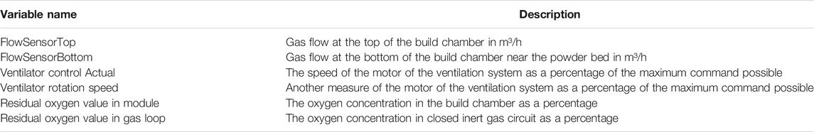
TABLE 1. Description of in-situ process data used to detect defects for this analysis.

Trajectory Data

In addition to the previously described temporal process data, spatial information from the laser modules is captured during the melt phase. This data is captured during a build by a National Instruments PXIe-data acquisition device at an approximate sampling rate of 40 kHz and stored in a TDMS file. The data that are included for each sample are scaled x and y location on the build plate, an indicator of which laser module is melting, and intensities from an on-axis photodiode. From the sequence of coordinates and sampling rate the absolute order and timing of the melt is known.

For this work, these data are transformed from the format described and interpreted as line segments. The start and end coordinates of these line segments are the coordinates of the current sample and the coordinates of the subsequent sample. Thus, we can derive a distance for each scan line, and since the sampling rate is constant, velocity can also be derived. Finally, the relative start time for each scan line since the beginning of the melt can also be found. This can be extended further to find the time elapsed since the beginning of the melt for any arbitrary location in the trajectory.

Also, for this work the photodiode data was only used to infer part boundaries and not as an input feature. Figure 3 shows a close up of a plot of trajectory where the color is from the photodiode data and shows the component boundaries. Determining the component boundaries allows for the analysis of only voxels that are melted and where process perturbations may affect the local material properties. This will be elaborated upon later in this paper. With the part boundaries identified, consecutive sub-scans could be consolidated into a single raster line. Table 2 shows the variable names and descriptions of the trajectory data.

FIGURE 3

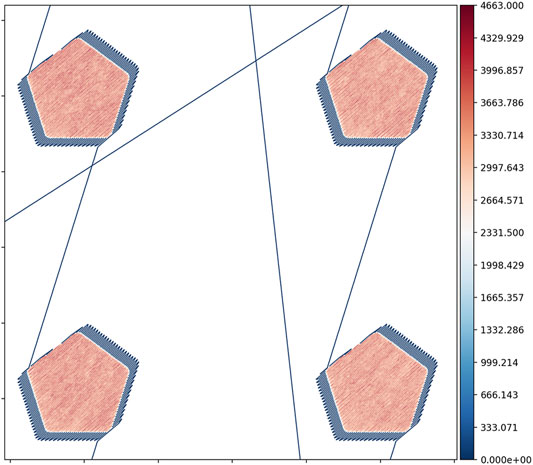
FIGURE 3. Example of trajectory data from build 1 zoomed in on four components. The image shows the melt areas, skywriting, and jump lines, and the visualized data are the raw digital intensity levels from the on-axis photodiode that was used to determine the component boundaries for spatial mapping.

TABLE 2

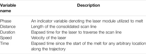
TABLE 2. Description of trajectory data used as the basis of spatial mapping of the in-situ process data and to detect defects for this analysis.

Defect Data

Finally, the defect data are generated from in-situ images of the powder bed that are collected by an off-axis, five-megapixel, visible light camera focused on the powder bed. The camera captures the full 245 × 245 mm build plate, and the build area is illuminated from above by an LED array (Scime et al., 2020). Two images are taken for each layer—one after powder spreading and another after the melt is complete.

The defect predictions are generated by Peregrine—a tool developed at ORNL (Scime et al., 2020). This tool uses a deep convolutional neural network (CNN)—what the authors specifically refer to as a dynamic segmentation convolutional neural network (DSCNN)—to perform semantic segmentation on the in-situ, layer-wise images. Semantic segmentation is a computer vision task for assigning one or multiple class labels to each pixel that is a constituent of an object within an image. As stated previously, we focus specifically on the “Soot” defect because this defect is generated during the melt and is influenced by build chamber gas flow and possibly by other process factors such as the laser trajectory and possibly amount of oxygen in the chamber—all features that are captured in the process log or trajectory data.

Peregrine outputs a categorical label for each voxel in a layer. Since only one label is investigated for this work, the defect data are transformed to a Boolean value indicating the presence of soot or not. Figure 4 shows the Boolean defect detections for a single layer as a binary image. Note that the authors state that the off-axis setup of the imaging system leads to differing effective resolutions across the build chamber (Scime et al., 2020).

FIGURE 4

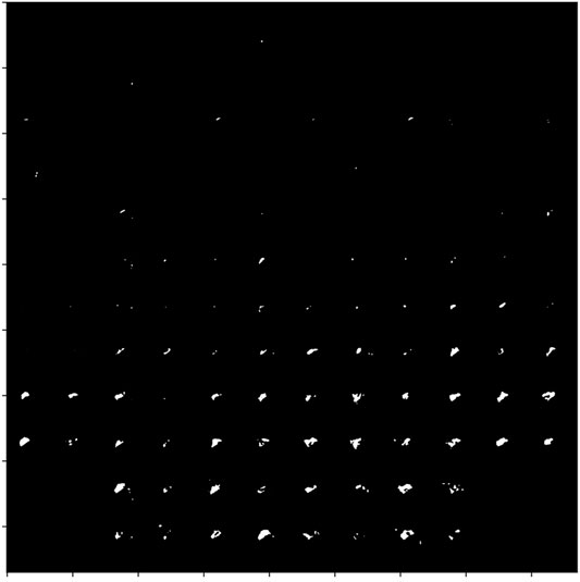
FIGURE 4. Binary class labels for “Soot” for each voxel of the build chamber in layer 10 of build 1 as predicted by Peregrine.

XGBoost Background

XGBoost is a fast and effective ML model implementation (Chen and Guestrin, 2016). It has been used effectively for many different, real-world applications—often achieving top performance for structured data tasks (Chen and Guestrin, 2016) (Awesome XGBoost, 2021).

Model Description

XGBoost is an implementation of Gradient Boosted Machine (GBM). GBM, in turn, is a robust ML model that aims to train many weak learners that, when leveraged in conjunction, act as one strong model (Friedman, 2001). A weak learner is a model whose predictions are only slightly better than random guessing; they are simple and typically have few learnable parameters. As such, GBM is an example of ensemble learning, and specifically as the name denotes, it implements a paradigm of ensemble learning called boosting. Boosted models are still trained using gradient descent; however, it differs from typical gradient descent training used in other, monolithic models such as logistic regression or neural networks. A brief discussion of similarities and differences between training GBM’s and other ML models that the reader may be familiar with is now presented. The equations are taken from the original paper on GBM’s by Friedman (Friedman, 2001) with minor simplifications for brevity and clarity.

The goal of supervised ML is to find an optimal function, F^*(x), minimizes a loss function, $\text{Ψ}$, with respect to provided labels or response values, y, as shown in Eq. 1.

${\mathit{F}}^{\ast }\left(\mathit{x}\right)=\mathit{arg}\underset{\mathit{F}\left(\mathit{x}\right)}{\min }{\mathit{E}}_{\mathit{y},\mathit{x}}\text{Ψ}\left(\mathit{y},\mathit{F}\left(\mathit{x}\right)\right)(1)$

Many different types of ML models have been developed to this end, and many of these models, such as logistic regression and neural networks, are parameterized. This means that finding an optimal function for a given model occurs when optimal model parameters, P^*, are found as shown in Eq. 2.

${\mathit{P}}^{\ast }=\mathit{arg}\underset{\mathit{P}}{\min }{\mathit{E}}_{\mathit{y},\mathit{x}}\text{Ψ}(\mathit{y},\mathit{F}\left(\mathit{x},\mathit{P}\right);{\mathit{F}}^{\ast }\left(\mathit{x}\right)=\mathit{F}\left(\mathit{x},{\mathit{P}}^{\ast }\right)(2)$

The optimization of the parameters occurs by updating the parameters over the course of M iterations from an initial guess, $p_0$, as shown in Eq. 3.

${\mathit{P}}^{\ast }={\displaystyle \sum _{\mathit{m}=0}^{\mathit{M}}{\mathit{p}}_{\mathit{m}}}(3)$

Each update is a small increment—scaled by a learning rate, $\alpha$—along the negative gradient of the loss function with respect to the current parameter values, as shown in Eqs 4, 5.

${\mathit{p}}_{\mathit{m}}=-\alpha {\mathit{g}}_{\mathit{m}}(4)$

${\mathit{g}}_{\mathit{m}}={\left[\frac{\partial \text{Ψ}\left(\mathit{y},\mathit{F}\left(\mathit{x},\mathit{P}\right)\right)}{\partial \mathit{P}}\right]}_{\mathit{P}={\mathit{P}}_{\mathit{m}-1}}(5)$

In fact, GBM’s leverage a similar algorithm for model training. As an ensemble method, the optimal function, F^*(x), is a summation of constituent weak learner models, and like conventional models, the optimization of this ensemble can be performed by iterative updates as shown in Eq. 6.

${\mathit{F}}^{\ast }\left(\mathit{x}\right)={\displaystyle \sum }_{\mathit{m}=0}^{\mathit{M}}{\mathit{f}}_{\mathit{m}}\left(\mathit{x}\right)(6)$

However, instead of updating one set of model parameters, the ensemble incrementally adds additional learners along the negative gradient of the ensemble loss with respect to all the current learners in the ensemble, as show in Eqs 7, 8.

${\mathit{f}}_{\mathit{m}}\left(\mathit{x}\right)=-\mathit{\rho }{\mathit{g}}_{\mathit{m}}\left(\mathit{x}\right)(7)$

${\mathit{g}}_{\mathit{m}}\left(\mathit{x}\right)={\mathit{E}}_{\mathit{y}}{\left[\frac{\partial \text{Ψ}\left(\mathit{y},\mathit{F}\left(\mathit{x}\right)\right)}{\partial \mathit{F}\left(\mathit{x}\right)}|\mathit{x}\right]}_{\mathit{F}\left(\mathit{x}\right)={\mathit{F}}_{\mathit{m}-1}\left(\mathit{x}\right)}(8)$

So, gradient boosting performs gradient descent by iteratively training additive models that each attempt to lower the global loss of the ensemble. For a complete technical description of the model and underlying algorithm, the reader is referred to original paper on GBM’s by Friedman (Friedman, 2001) as well as a technical overview provided in the XGBoost documentation (Introduction to Boosted Trees, 2021).

Typically, XGBoost employs decision trees as the base, weak learners; however, other base models may be used instead. Also, it may be used for either classification or regression. For this task we used the classification version with the decision tree base learner. The model has several user-defined parameters that affect training and performance of the algorithm. A subset of the parameters that are considered the most important are shown in Table 3. The values for these parameters were empirically optimized. This process is covered in Model parameter optimization and tuning Section.

TABLE 3

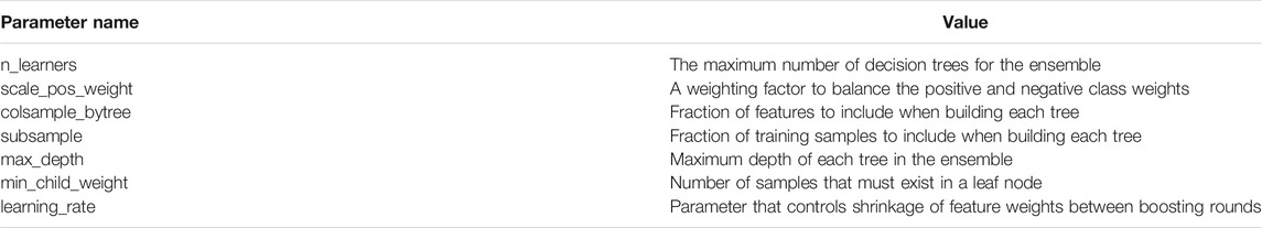
TABLE 3. Description of a subset of XGBoost model parameters.

Model Interpretability

Additionally, XGBoost offers several metrics for evaluating the importance of input features on the performance of the final model. This enables a user to gain a better understanding of the key relationships between the input features and the output. This is an important advantage over other, deep neural network ML models. Specifically, XGBoost offers three distinct metrics for feature importance: gain, weight, and cover (Pythone API Reference, 2021). The gain metric calculates the average improvement to the model’s loss contributed by each feature. Cover and frequency refer to how many samples are associated with a feature and how often a feature was utilized for splits within the ensemble respectively. Based on these definitions, gain is a more relevant evaluation metric when compared to the other two. Therefore, we focus on it to analyze the input features. This will allow for the investigation and initial determination of which process data may be most closely associated with the chosen defect class–soot.

Methodology

Before the analysis is possible on these data, several transformations and preprocessing steps must be performed. These steps are outlined here, but for the sake of brevity and scope some of the more technical details are omitted.

Temporal and Trajectory Data Transformation

The temporal data from the in-situ sensors as well as some of the trajectory data, and spatial data from the in-situ images and defect detections, are not immediately useful in conjunction. Indeed, typical data analysis is restrained to using each of these modalities only in isolation. As such, the need to transform one of these modalities to the other is necessary for them to be leveraged together. To this end and for this work, we propose a “spatial mapping” transformation that takes the inherently temporal in-situ process data and turns it into a spatial dataset.

Several items are needed to complete this transformation: an absolute timestamp for the start of the melt phase for each layer and the location and timing information of the heat source. For the ConceptLaser M2 these data come from the build log and the trajectory data respectively. The ultimate goal is to transform the temporal data into an image-like array of the same shape as the in-situ image data and Peregrine defect predictions.

The basic process is to use the location information from the trajectory data to determine which voxels each scan line travels through for a given layer. The timing information of the trajectory data gives the relative time from the start of the melt that the pixels are intersected by the laser. The melt start time given in the build log gives the absolute time for the start of the melt, and together yield the absolute time that the laser passed through each pixel. With this information, one can trivially index into the in-situ process data and pull any sensor value from a given time that corresponds to a physical location where the laser was melting material. Figure 5 illustrates this general concept. This spatial mapping and voxelization of the data can be performed for any arbitrary voxel resolution; however, intuitively, the data are mapped to match the resolution—approximately 100 µm—of the Peregrine defect prediction data.

FIGURE 5

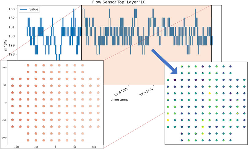
FIGURE 5. A sample layer from build 1 includes trajectory data, log data for “FlowSensorTop”, and the subsequent mapped data. The orange highlighted portion of the log data corresponds to the melt phase for the layer as indicated by the “Exposure started for” and “Exposure ended for” log file entries.

Once this data transformation is complete, the in-situ process data as well as the trajectory data are in the same domain as the defect data. Each voxel of each component contains localized in-situ process data, trajectory data from the laser scan path, as well as local defect detections.

Data Preprocessing

After the data are transformed to the same voxelized, spatial domain, as shown in Figure 6, several more preprocessing steps are performed before the analysis. These steps and rationale are outlined in this section.

FIGURE 6

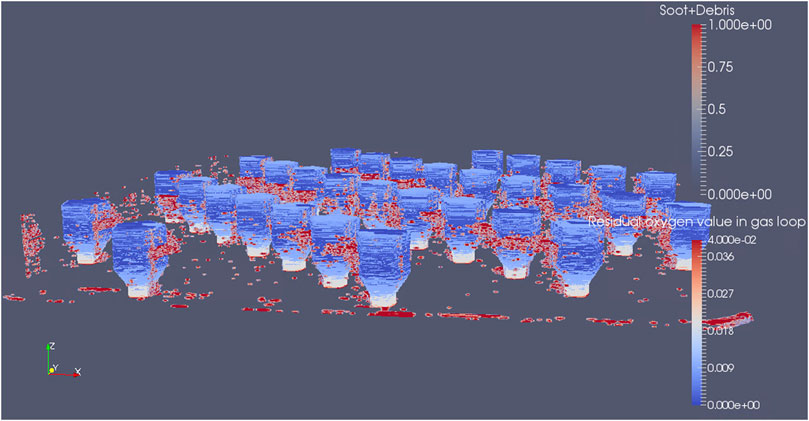
FIGURE 6. 3D plot of the build volume of spatially mapped process data for “Residual oxygen value in gas loop” with defects overlaid for build 2. Note that this image shows combined soot and debris defects (Scime et al., 2020), but for the actual analysis only soot was considered.

Defect Data Preprocessing

First, the defect data undergo a dilation operation. Through qualitative analysis it was determined that many of the “Soot” defect detections occurred over the powder bed and proximal to the printed components with vanishingly few detections over the components themselves. This operation expands the defect predictions from the original set of voxels to adjacent voxels, and it serves to reasonably increase the number of “Soot” voxels that intersect with voxels where mapped process data exist. The likely reality is that the soot particles are also present on the printed surfaces in quantities proportional to their presence near the part; however, the imaging conditions make their on-part in-situ detection challenging.

Full Data Preprocessing

The next operation is a Gaussian blur of defects and in-situ process data—both the log data and the trajectory data. Within the AM process, many complex interactions occur within local regions, so this Gaussian blurring of the data serves to blend the data together and eliminate hard boundaries between defects and nominal voxels as well as voxels with one sensor value proximal to another with a different value from the same sensor.

Afterwards, the data were resized spatially to reduce the data burden. This decreased the voxel spatial resolution of the data from 100 × 100 µm to 300 × 300 µm. This was determined to be a reasonable processing step since soot may be detected from in-situ layer images at lower resolutions.

The blurring and resizing of the data create a target set, “Soot”, that is no longer simply 0’s and 1’s, so we threshold the defect data of the lower resolution dataset at 0.5 to recreate a Boolean target for classification.

Now the data are in a form where many voxels in the build chamber contain data from all three data sources (any voxel outside the geometry where no in-situ process data exist is removed). This dataset is now appropriate for training a supervised ML model. Each voxel represents a sample in the dataset with process and trajectory data acting as the input features and the defect labels serving as the training targets.

Several final preprocessing steps are taken. Namely, the removal of some bad data points. Specifically, these were voxels where the trajectory “Speed” value had been corrupted at some point along the way and had a value of infinity. This represented a very small number of overall voxels.

At this point a subset of the data was generated by randomly choosing one million voxels with spatially mapped data from each of the four builds. For the first build this represented approximately 1.5% of the voxels, and for the remaining three builds it represented approximately 6%. This subset of the data were used for parameter optimization, as outlined later in the paper, and for final model training.

Finally, the input features were duplicated, standardized in two different ways, and concatenated to create the final input feature set. The first copy of input features was each standardized globally across all four builds. For each feature a global mean and standard deviation were calculated. Then for each sample, each respective feature was zero centered and scaled to have a unit standard deviation. The second copy of input features were standardized per build—meaning that the mean and standard deviation were calculated for each feature and build separately and then each sample was standardized based upon which build it belonged to. The rationale for these two, simultaneous standardization methods is that the global standardization will allow a ML algorithm to learn important trends and relationships in the absolute ranges for each sensor. The build-wise standardization, on the other hand, will help account for and mitigate any possible sensor drift or changes in calibration between builds and still allow for the ML algorithm to learn relationships between changes in relative sensor values and defects.

Model Parameter Optimization and Tuning

ML models have distinct parameters that affect the training characteristics and performance of the model. For this work we approximately followed the parameter optimization procedure as outlined in (Aarshay, 2016), and we only optimized the parameters discussed in Model Description Section. Parameters of interest were set to default values as outlined in the XGBoost documentation until optimized with one exception. The “scale_pos_weight” value was initialized using a heuristic recommended by the creators of XGBoost—a ratio of the number of negative samples to the number of positive samples (XGBoost Parameters, 2021).

Additionally, receiver operating characteristic (ROC) area under the curve (AUC) is used as the evaluation metric during parameter optimization. It was chosen because it is well suited for binary classification tasks when there is a significant class imbalance. Using this evaluation metric mandates that the model use logistic regression as its objective to perform the classification (XGBoost Parameters, 2021).

To determine the model performance more accurately for a given parameter set, the dataset is typically divided into multiple folds, or training and validation set pairs, that are each used to evaluate the model performance and across which an average performance is calculated in a process called cross validation. For this work, the voxels were divided into four folds each consisting of approximately four million voxels. The validation set of each fold contained voxels from only one of the four builds—one million voxels; the training set contained the remaining voxels from the other three builds—three million voxels. This was done to emulate a likely scenario where an ML model is trained on data from existing builds and then used to predict properties of new builds. Later, for model training this same principle was applied—models were trained on data from three builds to predict defects for the fourth build.

The first optimization was to determine an initial number of learners, n_learners. An XGBoost model was trained with an initial goal of 1,000 learners; however, early stopping was enabled that would end training after 50 consecutive trees failed to reduce the loss and the number of learners with the best average loss across the four folds was used.

Next, with the new number of learners established, “scale_pos_weight” was optimized from its original, heuristic-based number. This optimization was done by using random search as implemented in the python library scikit-learn (Pedregosa et al., 2011). Twenty randomly selected values between the square root of “scale_pos_weight” and the original, heuristic-base “scale_pos_weight” were tested while holding the remaining model parameters constant. A second random search of a narrower range was performed if it was deemed necessary.

Then, “max_depth” and “min_child_weight” were jointly optimized followed by another round of updates to “n_learners”. Afterwards, “colsample_bytree” and “subsample” were jointly optimized. Finally, “learning_rate” was manually set to 0.01 and the final value for “n_learners” was determined. The optimized model parameter values are shown in Table 4. An asterisk indicates that the parameter was chosen manually and did not undergo any optimization.

TABLE 4

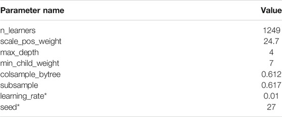
TABLE 4. Final XGBoost model parameters used to train all models for analysis.

Input Feature Subsets

Several different subsets of the features were used to train models (each using the same model parameters previously outlined). This ablation study was performed to establish the effect on model performance that different in-situ data had for identifying defects. These subsets were as follows: the full feature set—both in-situ sensor data and trajectory data, the full feature set excluding the ordering information from the trajectory data, and finally a subset that consisted only of in-situ sensor data and laser module data. Table 5 shows these three different input feature sets. Recall that each feature listed, except “Phase”, actually represents two input features—one that is globally standardized and another that is standardized per build.

TABLE 5

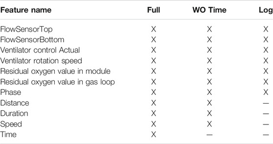
TABLE 5. Three different input feature sets (“Full”, “Without Time”, and “Log Data”) that were used to train the XGBoost model.

These subsets were chosen with the following respective rationales: to train a model on a comprehensive feature set that did not include any explicit location information, to train a model on a feature set that did not include implicit location information (in the form of scan path order as given in the “Time” feature), and to train a model strictly on in-situ process data and establish initial relationships between these signals and detected defects. Note that “Phase”—information about which laser module was melting—was included in all three feature sets because the log files also indicate when each laser is being utilized. In summary, a total of twelve models were trained—four models trained on data from three builds to predict defects in the fourth and replicated for all three subsets of the feature set.

Results

Models were trained with the optimized XGBoost model parameters. One model was trained to make voxel-level soot predictions for each of the four builds with sampled data from the other three builds—approximately three million voxels worth of data. This was repeated for each of the three distinct input feature sets. This process produced several distinct results that will each be presented. The overall performance of each model, the feature importance rankings for each model, and the location-based performance for each model will be presented.

Model Performance

Confusion matrices are a canonical way of presenting classification results; however, the imbalanced nature of this problem makes their use impractical because the overwhelming majority of predictions are true negatives. Instead, we will discuss several metrics in conjunction that will allow for analyzing the model performances. These are sensitivity and specificity, balanced accuracy, as well as false omission rate and false discovery rate.

Sensitivity is also known as the true positive rate and is the fraction of ground-truth positives that were correctly predicted as a percentage of all ground-truth positive examples. Similarly, specificity is also known as the true negative rate and is the fraction of ground-truth negatives that were correctly predicted as a percentage of all ground-truth negative samples. Balanced accuracy is the average of sensitivity and specificity and is a good metric for analyzing performance in light of class imbalance. False omission rate is the fraction of data that were ground-truth positive that were incorrectly predicted as a percentage of all model-predicted negatives; false discovery rate is the fraction of data that were ground-truth negative that were incorrectly predicted as a percentage of all model-predicted positives. Table 6 shows the performance for all twelve models as well as aggregated metrics across the four build-wise models for each input feature set.

TABLE 6

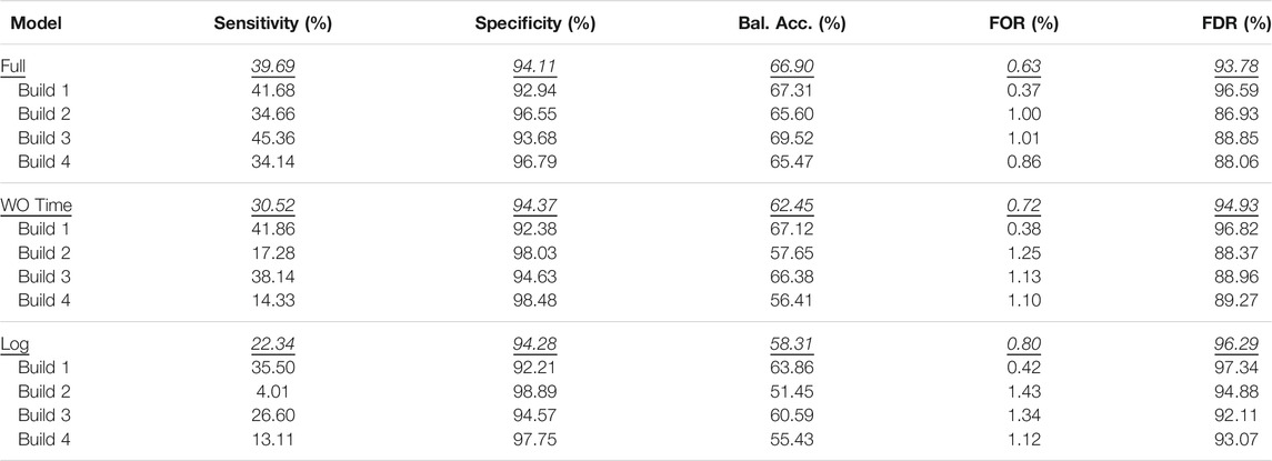
TABLE 6. Model performances. The top lines for each input feature set represents the aggregated performance across all four models and respective builds.

Feature Importance

As previously discussed, XGBoost offers metrics for ranking the importance of each feature for producing predictions. Figure 7 shows the top ten features for each of the twelve models divided up by input feature sets.

FIGURE 7

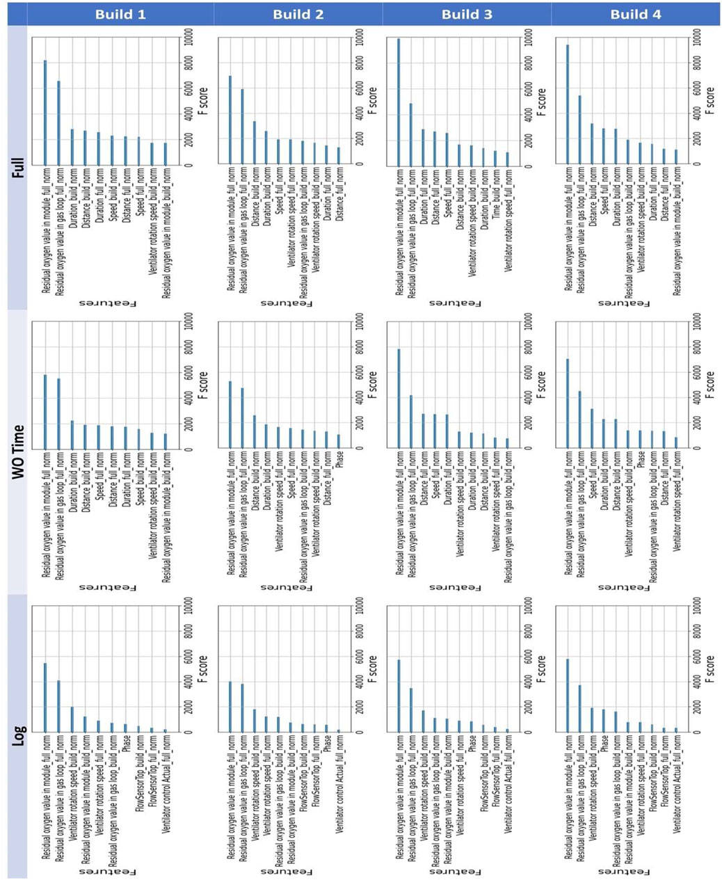
FIGURE 7. XGBoost feature importances for the twelve build and dataset combinations.

Location-Based Model Performance

The performance results can also be calculated per component and visualized. This may lead to some interesting observations about the model performance. Figure 8 show the component-wise balanced accuracy for each build and input feature set. Note that the coloring scale is not consistent across the images. This was done to ensure that differences among the components and trends across the build chamber could be observed easily. Also, note that changes in balanced accuracy are dominantly influenced by changes in the sensitivity metric across the build chamber.

FIGURE 8

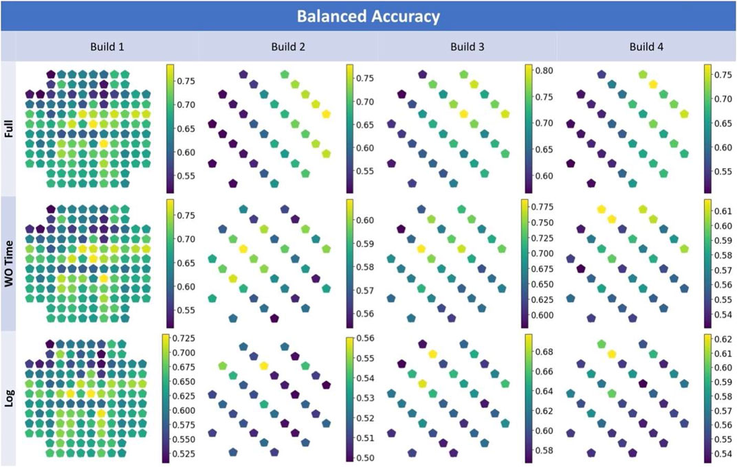
FIGURE 8. Visualization of balanced accuracy per component of each build for the “Log” input feature set.

For context, the spatial distribution of the soot prevalence per build is shown in Figure 9.

FIGURE 9

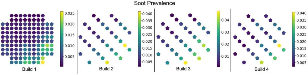
FIGURE 9. Spatial distribution of soot prevalence for the four builds.

Discussion

Analysis

The results from this analysis show fair performance but with ample room for improvement with respect to the various metrics. The model achieved an aggregated best sensitivity of approximately 40% and balanced accuracy of approximately 67%. However, the model still performed better than a baseline of random guessing. In general, models for builds 1 and 3 had better performance. Additionally, the performance consistently decreased with more restricted input feature sets.

Across all twelve XGBoost models, two input features were consistently measured to have the greatest importance for model predictions across all builds and input feature sets. These were “Residual oxygen value in module_full_norm” and “Residual oxygen value in gas loop_full_norm” constantly occupying the first and second positions respectively. This makes strong intuitive sense as increasing levels of oxygen lead to greater levels of oxidation on the exposed surface that manifest as darker regions that are easy for Peregrine to detect as soot. Additionally, these two features were the globally standardized versions (indicated by the “_full_norm” suffix), so it is the absolute ranges for residual oxygen that is most informative (as opposed to the relative changes within a relative range in the sensor readings within a build).

Finally, several interesting spatial trends are observed when visualizing model performance in different regions of the build area—especially as observed in builds 2-4. Figure 9 shows how the prevalence of soot increases toward the front of the build chamber. The prevalence is also skewed toward the right side of the build chamber. When “Time” is included as an input feature, the XGBoost models likely consistently uses it to approximately determine location. This occurs because the ConceptLaser M2 machine printed these components at the extreme left side of the machine first proceeding from front to back. The “Time” feature indirectly gives the model approximate spatial information. As such, the models are able to correctly predict more samples on the right side of the machine where the prevalence is greater as shown in the first row of Figure 8—labelled “Full”. However, when the “Time” feature is removed, performance across the build plate changes. Row two of Figure 8—labelled “WO Time”—shows that the balanced accuracy tends to be greater toward the back of the build chamber albeit only slightly. This may stem from the data lacking information that relates to the higher prevalence of soot at the front of the build chamber leading to decreased model sensitivity. Using only in-situ process log data shows a similar pattern. Across all three input feature sets, the component-wise balanced accuracy is very similar for build 1. This is likely related to the models that predicted defects for build 1 having been trained on builds 2 through 4 that have a different geometry. Since different geometries yield different trajectory data, the model was likely unable to leverage those features effectively for defect detection and thus the little apparent spatial performance change from one input feature set to the next.

Future Work

This work demonstrates a first take on leveraging already-available in-situ process and trajectory data modalities, but it only begins to scratch the surface of testing the possible utility of these data. When training the ML model this work completely neglected spatial information and makes predictions for each voxel based only on the sensor values for that voxel. Instead of XGBoost these data could be used to train a deep CNN which would be able to learn from the spatial relationships between the mapped voxels in addition to the mapped data. Further, they could be employed as additional input channels in existing deep learning NN models, like the DSCNN that generated the initial defect data in this study, for more accurate defect detection. Alternatively, with spatial and trajectory data omitted, as was the case for the third input feature set, the existing models could be utilized directly with sampled, streaming in-situ process data to make defect predictions in real-time as a coarse AI-based process monitoring system.

Finally, this type of analysis should be readily employable for any AM technology that has the requisite data—in-situ temporal process data, trajectory data, and localized property data. One can even imagine leveraging this method to mine for relationships between other localized properties such as microstructure and mechanical properties by utilizing the feature importance scores produced by XGBoost to discover relationships between the inputs and targets to investigate further with targeted experiments.

Conclusion

This analysis represents a first attempt at leveraging in-situ process data for predicting localized build defects. It elicits interesting possibilities for leveraging temporal data modalities for predicting localized spatial properties. Specifically, that spatially mapped, in-situ process and trajectory data may be fused into a common representation and related to image-based defect data. The overall performance of the model is likely not adequate to be deployed as the sole means for process monitoring and soot detection. However, the use of XGBoost as the chosen classifier yields desirable auxiliary capabilities—namely the ability to narrow down which in-situ data are most relevant for detecting certain in-situ defects. Additionally, the spatially transformed in-situ process dataset may be used as additional inputs to other ML models for more accurate prediction of defects.

Data Availability Statement

The raw data supporting the conclusions of this article will be made available by the authors, without undue reservation.

Author Contributions

WH contributed to ideation and implementation—including data processing, data analysis, and interpretation of results—and drafted the manuscript. DR assisted in ideation and made intellectual contributions toward optimizing, training, and evaluating the ML model and reviewed the manuscript. LS assisted in ideation and made intellectual contributions toward spatial mapping of process data as well as interpreting the results and provided domain expertise regarding the data and reviewed the manuscript. RD assisted in ideation and made intellectual contributions toward spatial mapping of process data and provided the build data that was used for analysis. VP assisted in ideation and made intellectual contributions toward spatial mapping of process data and provided funding for the work.

Funding

This manuscript has been authored by UT-Battelle, LLC, under contract DE-AC05-00OR22725 with the U.S. Department of Energy (DOE). DOE will provide public access to these results of federally sponsored research in accordance with the DOE Public Access Plan (https://energy.gov/downloads/doe-public-access-plan). Research was sponsored by the U.S. Department of Energy, Office of Energy Efficiency and Renewable Energy, Advanced Manufacturing Office.

Conflict of Interest

The authors declare that the research was conducted in the absence of any commercial or financial relationships that could be construed as a potential conflict of interest.

Publisher’s Note

All claims expressed in this article are solely those of the authors and do not necessarily represent those of their affiliated organizations, or those of the publisher, the editors and the reviewers. Any product that may be evaluated in this article, or claim that may be made by its manufacturer, is not guaranteed or endorsed by the publisher.

Acknowledgments

Additionally, the authors would like to thank Michael Sprayberry and Joseph Simpson of ORNL for their technical review of this manuscript.

References

Aarshay, J. (2016). “Complete Guide to Parameter Tuning in XGBoost.” Analytics Vida. [Online]. Available: https://www.analyticsvidhya.com/blog/2016/03/complete-guide-parameter-tuning-xgboost-with-codes-python/.

Google Scholar

“Awesome XGBoost.”(2021) [Online]. Available: https://github.com/dmlc/xgboost/tree/master/demo#machine-learning-challenge-winning-solutions. [Accessed: 10-Aug-2021].

Google Scholar

Chandrasekar, S., Coble, J. B., Yoder, S., Nandwana, P., Dehoff, R. R., Paquit, V. C., et al. (2019). Investigating the Effect of Metal Powder Recycling in Electron Beam Powder Bed Fusion Using Process Log Data. Addit. Manuf. 32, 100994. doi:10.1016/j.addma.2019.100994

CrossRef Full Text | Google Scholar

Chen, T., and Guestrin, C. (2016). XGBoost: A Scalable Tree Boosting System” in Proceedings Of the 22nd Acm Sigkdd International Conference on Knowledge Discovery and Data Mining, 785–794.

Google Scholar

DebRoy, T., Wei, H. L., Zuback, J. S., Mukherjee, T., Elmer, J. W., Milewski, J. O., et al. (2018). Additive Manufacturing of Metallic Components - Process, Structure and Properties. Prog. Mater. Sci. 92, 112–224. doi:10.1016/j.pmatsci.2017.10.001

CrossRef Full Text | Google Scholar

Everton, S. K., Hirsch, M., Stravroulakis, P., Leach, R. K., and Clare, A. T. (2016). Review of In-Situ Process Monitoring and In-Situ Metrology for Metal Additive Manufacturing. Mater. Des. 95, 431–445. doi:10.1016/j.matdes.2016.01.099

CrossRef Full Text | Google Scholar

Friedman, J. H. (2001). Greedy Function Approximation: a Gradient Boosting Machine. Ann. Stat. 2, 34. doi:10.1214/aos/1013203451

CrossRef Full Text | Google Scholar

Grasso, M., and Colosimo, B. M. (2017). Process Defects and In Situ Monitoring Methods in Metal Powder Bed Fusion: A Review. Meas. Sci. Technol. 28 (4). doi:10.1088/1361-6501/aa5c4f

CrossRef Full Text | Google Scholar

Grasso, M., Gallina, F., and Colosimo, B. M. (2018). Data Fusion Methods for Statistical Process Monitoring and Quality Characterization in Metal Additive Manufacturing. Proced. CIRP 75, 103–107. doi:10.1016/j.procir.2018.04.045

CrossRef Full Text | Google Scholar

Heiden, M. J., Deibler, L. A., Rodelas, J. M., Koepke, J. R., Tung, D. J., Saiz, D. J., et al. (2019). Evolution of 316L Stainless Steel Feedstock Due to Laser Powder Bed Fusion Process. Additive Manufacturing 25, 84–103. doi:10.1016/j.addma.2018.10.019

CrossRef Full Text | Google Scholar

Herderick, E. (20112011). Additive Manufacturing of Metals: A Review. Mater. Sci. Technol. Conf. Exhib.MS T’11 2 (176252), 1413.

Google Scholar

Huang, D. J., and Li, H. (2021). A Machine Learning Guided Investigation of Quality Repeatability in Metal Laser Powder Bed Fusion Additive Manufacturing. Mater. Des. 203, 109606. doi:10.1016/j.matdes.2021.109606

CrossRef Full Text | Google Scholar

Introduction to Boosted Trees,”(2021) XGBoost. [Online]. Available: https://xgboost.readthedocs.io/en/latest/tutorials/model.html. [Accessed: 05-Oct-2021].

Google Scholar

Kok, Y., Tan, X. P., Wang, P., Nai, M. L. S., Loh, N. H., Liu, E., et al. (2018). Anisotropy and Heterogeneity of Microstructure and Mechanical Properties in Metal Additive Manufacturing: A Critical Review. Mater. Des. 139, 565–586. doi:10.1016/j.matdes.2017.11.021

CrossRef Full Text | Google Scholar

Lou, X., and Gandy, D. (2019). Advanced Manufacturing for Nuclear Energy. Jom 71 (8), 2834–2836. doi:10.1007/s11837-019-03607-4

CrossRef Full Text | Google Scholar

Moltumyr, A. H., Arbo, M. H., and Gravdahl, J. T. (2020). Towards Vision-Based Closed-Loop Additive Manufacturing : A Review.

Google Scholar

Pedregosa, F., Varoquaux, G., Gramfort, A., Michel, V., Thirion, B., et al. (2011). Scikit-learn: Machine Learning in Python. J. Mach. Learn. Res. 12 (85), 2825–2830.

Google Scholar

Python API Reference.”(2021) [Online]. Available: https://xgboost.readthedocs.io/en/latest/python/python_api.html#module-xgboost.plotting. [Accessed: 11-Aug-2021].

Google Scholar

Roidl, B. “Continuous Improvement in Gas Flow Design,” Gas Flow White Pap.

Sames, W. J., List, F. A., Pannala, S., Dehoff, R. R., and Babu, S. S. (2016). The Metallurgy and Processing Science of Metal Additive Manufacturing. Int. Mater. Rev. 61 (5), 315–360. doi:10.1080/09506608.2015.1116649

CrossRef Full Text | Google Scholar

Scime, L., Siddel, D., Baird, S., and Paquit, V. (2020). Layer-wise Anomaly Detection and Classification for Powder Bed Additive Manufacturing Processes: A Machine-Agnostic Algorithm for Real-Time Pixel-wise Semantic Segmentation, Additive Manufacturing, 36. March, 101453. doi:10.1016/j.addma.2020.101453

CrossRef Full Text | Google Scholar

Steed, C. A., Halsey, W., Dehoff, R., Yoder, S. L., Paquit, V., Powers, S., et al. (2017). Falcon: Visual Analysis of Large, Irregularly Sampled, and Multivariate Time Series Data in Additive Manufacturing. Comput. Graphics 63, 50–64. doi:10.1016/j.cag.2017.02.005

CrossRef Full Text | Google Scholar

Vandone, A., Baraldo, S., and Valente, A. (2018). Multisensor Data Fusion for Additive Manufacturing Process Control” IEEE Robot. Autom. Lett.

Google Scholar

“XGBoost Parameters.” (2021) [Online]. Available: https://xgboost.readthedocs.io/en/latest/parameter.html. [Accessed: 10-Aug-2021].

Google Scholar