Variational Approach to Damage Induced by Drainage in Partially Saturated Granular Geomaterials

1 Introduction

How can mode-I fractures initiate on the surface of saturated granular geomaterials which are under compressive effective stress states when subjected to forced drainage or drying boundary conditions? This question has been intriguing some researchers for the last decade especially in the light of the prevailing assessment that in homogeneous desiccating soils, macroscopic surface cracks can appear only in the presence of tensile stresses induced by zero displacement boundary conditions or by moisture gradients through the thickness of the sample capable of inducing nontrivial stress concentration, see for example Peron et al. (2009); Cordero et al. (2021). Indeed, following Shin and Santamarina (2010, 2011), a different mechanism can be invoked to explain opening-like fractures appearing at the drained/drying surface of uncemented granular materials, which is compatible with their fundamental behavior to exhibit a cohesive state only under compressive effective stresses. In this case, fracturing is hypothesized to be caused by the forced invasion of the pore network by either immiscible or miscible fluids. In the study by Shin and Santamarina (2010) water-saturated slurry of clay in a cylindrical chamber was subjected to pressure by a superposed immiscible nonwetting fluid (oil). This is a scenario which unambiguously generates compressive effective stresses within the confined sample with the ratio of horizontal to vertical effective stresses less than 1, which is typical of granular media. Drainage was initiated by opening a port below the sample. Following an initial settlement of the sediment, mode-I fracture initiation was observed at sub-millimeter defects on the invasion surface, and these fractures propagated vertically downward and laterally within a plane normal to the minor principal effective stress. This definitely cannot be explained through a tensile stress–driven mechanism. In Shin and Santamarina (2010, 2011), it has been hypothesized that such fracture initiation and the initiation of pattern-forming surface fractures typical to desiccating soils are due to capillary pressure overwhelming the maximum pressure that a granular material can resist before a new fluid–fluid interface is formed. In a more recent publication, Cordero et al. (2017), the effects of suction and compressibility of the overall granular material on desiccation fracture formation have been discussed. A similar configuration has also been investigated using the Discrete Element Method by Jain and Juanes (2009); in this case, however, a local condition for fracture opening has been identified, on the basis of classical fracture mechanics, requiring the gas pressure to exceed the minimum compressive stress.

Looking at the macroscopic modeling of such behavior of granular geomaterials, few contributions can be retrieved from the literature assuming brittle fracture to be allowed under tensile stresses and shear stresses. We refer among others to Peron et al. (2013) and to those approaches that even model the fracture nucleation/propagation, for instance, the phase-field approaches proposed by Choo and Sun (2018); Cajuhi et al. (2018) and references therein. However, these approaches are not adapted to model the triggering of opening-like fractures under purely compressive effective stresses on the surface of saturated granular materials when subjected to forced drainage or drying boundary conditions. This is the reason why a new phase-field model is proposed here, which assumes the micro-scale grain reorganization to not affect the macroscopic stiffness of the material but its retention properties, hence allowing for the characterization of a damage criterion comparing a given threshold with the released capillary energy rather than with the elastic one. On the other hand, it is to be noted that rock-like geomaterials are known (Zhou, 2005, 2006; Zhou et al., 2008; Spetz et al., 2021) to exhibit, under overall compressive loading, a dilatation of pre-existing defects leading to their further opening-mode propagation. However, the current work is neither intended to describe such materials/geometry nor such loading scenarios.

This work is organized as follows. The proposed approach is presented in Section 2. Section 3 is devoted to presenting the numerical algorithm implementing the aforementioned phase-field approach, while in Section 4, the desiccation problem is formulated and solved, discussing the stability of damage profiles and their capability to induce damage localization. Conclusions and perspectives are briefly drawn in Section 5.

2 Mathematical Model

2.1 A Damaged Porous Solid

The partially saturated porous medium is described here adopting the classical approach of continuum poromechanics as presented by Coussy (2004), to which we refer for a detailed presentation; the notation used hereafter is consistent with that of the aforementioned reference. According to this classical approach to partial saturation, a porous solid is understood as a so-called ‘wetted’ porous skeleton with a thin layer of fluid attached to the pore walls, and thus a contribution to the stored energy of the porous solid is attributed to the fluid–fluid and solid–fluid interfaces. This interfacial energy density is obtained as the cumulative work carried out by a macroscopic capillary pressure difference between the wetting and the nonwetting fluids in modifying the relative fluid volume fractions within the pores.

Now, the formation of a fracture due to grain/pore reorganization, as hypothesized by Shin and Santamarina (2010, 2011), results in a discontinuity of the porous material. This “absence” of porous material within a fracture would mean, locally, a complete loss of retention property toward the wetting fluid and thus a loss of the ability of the porous medium to store interfacial energy. In the current study, a scalar damage variable, α, is introduced in order to describe the effects of grain/pore reorganization within the porous solid, in the regime of compressive effective stresses, as briefly discussed in the Introduction. Damage is thus assumed to induce a reduction in the air-entry pressure and in general to degrade the retention properties of the porous medium, which is equivalent to a reduction of the cumulative interfacial energy stored.

Accordingly, the degraded retention relation between the saturation degree of the wetting fluid, S_w, and the degraded macroscopic capillary pressure, p_c, reads,

$p_c\left(S_w,\alpha \right)=a\left(\alpha \right){\tilde{p}}_c\left(S_w\right)\approx -a\left(\alpha \right){\tilde{p}}_w\left(S_w\right)=-p_w\left(S_w,\alpha \right),(1)$

where a(α) is a damage law whose functional form is elaborated at a later point. p_w is the pore-pressure of the wetting fluid in a degraded porous solid, and ${\tilde{p}}_w$ its nondegraded counterpart. ${\tilde{p}}_c(S_w)$ represents the standard retention relation, unaffected by damage. In the current study, the widely used van Genuchten form (van Genuchten, 1980),

${\tilde{p}}_c\left(S_w\right)=\frac{{\rho }_{w}g}{{\alpha }_{vG}}{\left(S_w^{\frac{n}{1-n}}-1\right)}^{\frac{1}{n}},(2)$

is assumed where, α_vG and n are the model parameters, g is the acceleration due to gravity, and ρ_w is the mass density of liquid water. It is to be noted that residual saturation is assumed to be vanishing for simplicity but its incorporation is trivial.

Also, the assumptions leading to Richards’ equation (Hilfer and Steinle, 2014) are adopted, in particular the hypothesis of a passive non-wetting phase is assumed, leading to p_c ≈ −p_w in Eq. 1. While the above development serves as a reasonable first assumption for investigation, a complete modeling approach should also involve the degradation of the resistance to fluid flow within the damaged zone and eventually along localized fracture planes. With the abovementioned assumptions, the transient hydraulic problem governing the evolution of pore-pressure, p_w, within the porous solid is written as,

$\frac{\partial \left(\varphi S_w\right)}{\partial t}-\frac{\mathit{\varkappa }}{{\eta }_w}\nabla \cdot \left[K_{rw}\left(p_w\right)\left(\nabla p_w\right)\right]=0,(3)$

where the intrinsic permeability ϰ is assumed to be independent of α and ${\eta }_w$ is the dynamic viscosity of water. Since ϰ is expected to increase, in orders of magnitude, within a fracture, we make a rather simplifying assumption on the relative permeability function, K_rw(p_w) = 1 to in part compensate for the lack of the aforementioned coupling. It is to be noted that since the primary unknown factor in the aforementioned equation is the pore-pressure, S_w can then be derived from it using the degraded inverse retention relation,

$S_w\left(p_w,\alpha \right)={{\tilde{p}}_c}^{-1}\left(\frac{-p_w}{a\left(\alpha \right)}\right).(4)$

Appropriate boundary conditions compliment the aforementioned partial differential equation (PDE) which could be either an imposed flux representing a natural boundary condition or an imposed pressure representing a Dirichlet boundary condition.

We consider an n_d-dimensional domain, $\mathrm{\Omega }\in R^{n_d}$, representing the initial configuration of a damaging isotropic partially saturated porous solid whose boundary is denoted by ∂Ω. In line with standard gradient damage modeling (Marigo et al., 2016) and the theory of unsaturated poroelasticity, the following considerations are carried out.

1) The scalar internal variable, α ∈ [0, 1], is assigned the role of describing the extent of damage in the sense of loss of retention properties. α = 0 denotes an intact healthy skeleton whose retention properties are described by the standard retention curve, whereas α = 1 denotes a fully damaged skeleton whose retention properties are degraded and can only hold vanishing or residual amounts of wetting fluid.

2) For a given unit volume of porous solid in its reference configuration, the bulk energy density, W, accounting for the internal energy and the dissipation due to material degradation, is a state function characterized by $\partial \Omega$ (ɛ, ϕ, S_w, α, ∇α), respectively, the linearized strain tensor, the Lagrangian porosity, the saturation degree of the wetting fluid, the damage variable, and the damage gradient vector field.

3) In a similar way as the construction of the standard gradient damage model (Marigo et al., 2016) for the solid continuum, the porous solid is assumed to be dissipative in a nonlocal sense due to the dependency of the bulk energy density on the gradient of damage. The particular expression of the bulk energy density is assumed to be

$W\left(\epsilon ,\varphi ,S_w,\alpha ,\nabla \alpha \right)={\mathrm{\Psi }}_s\left(\epsilon ,\varphi ,S_w,\alpha \right)+w\left(\alpha \right)+\frac{1}{2}{w}_1{\ell }^2\nabla \alpha \cdot \nabla \alpha .(5)$

The different terms of the aforementioned expression are explained below.

a) The energy density of the porous solid, Ψ_s(ɛ, ϕ, S_w, α), encompasses the contributions due to the deformation of the porous skeleton, resulting in solid strains and changes in porosity and, also, the interfacial energy contribution due to formation/annihilation of interfaces. Adopting the concept of energy separation (Coussy, 2004) between the free energy of the porous skeleton and the interfacial energy we obtain,

${\mathrm{\Psi }}_s\left(\epsilon ,\varphi ,S_w,\alpha \right)={\psi }_s\left(\epsilon ,\varphi \right)+\varphi U\left(S_w,\alpha \right).(6)$

Here, a specific choice is made that would result in the aforementioned postulate that damage means the degradation of only the retention properties and not the poroelastic properties. The latter would have been the choice for modeling tensile mode fracture as carried out, for instance, by Cajuhi et al. (2018). The choice made here allows to isolate the investigation of fracture formation just due to the ‘release’ of interfacial energy. Specifically, we assume a degradation of the form,

$U\left(S_w,\alpha \right)=a\left(\alpha \right)\tilde{U}\left(S_w\right),(7)$

consistent with the definition of the degraded capillary pressure in Eq. 1. In Figure 1, the two functions p_c(S_w, α) and U(S_w, α) are depicted with the assumed degradation behavior. $\tilde{U}(S_w)$ represents the undamaged interfacial energy given by,

$\tilde{U}\left(S_w\right)={\int }_{S_w}^1{\tilde{p}}_c\left(s\right)ds.(8)$

FIGURE 1

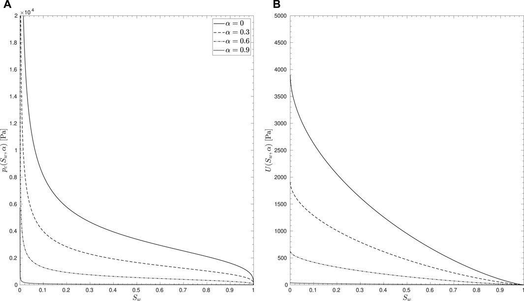
FIGURE 1. Proposed degradation of the retention properties with evolution of damage depicted for material properties taken from Table 1, (A) macroscopic capillary pressure, p_c(S_w, α), in Eq. 1, (B) interfacial energy density, U(S_w, α), in Eq. 7.

While various choices of the functional form of a(α) are possible, we make a specific choice following the standard gradient damage modeling,

$a\left(\alpha \right)={\left(1-\alpha \right)}^2+k_{\ell },(9)$

where k_ℓ is a small positive constant used solely for numerical purposes to govern the fully damaged state. Accordingly, when α grows from 0 to 1, the interfacial energy density degrades to a vanishing value. The consequence on the damage evolution due to the abovementioned choices is discussed further.

Now concerning the free energy density of the skeleton, a possible form that retrieves back the classical Biot’s linear constitutive relations as its state equations reads as,

${\psi }_s\left(\epsilon ,\varphi \right)=\frac{1}{2}{\mathbb{C}}^0\left(\epsilon -{\epsilon }_0\right)\cdot \left(\epsilon -{\epsilon }_0\right)+\frac{1}{2}{b}^{2}N{\left(ϵ-{ϵ}_0\right)}^2-\mathrm{\Delta }\varphi \left(bN\left(ϵ-{ϵ}_0\right)-p_0^{\ast }\right)+\frac{1}{2}N\mathrm{\Delta }{\varphi }^2,(10)$

where the notations are borrowed from Coussy (2004). ${\mathbb{C}}^0$ is the elastic stiffness tensor, b the Biot coefficient, and N the tangent Biot modulus. Δϕ represents the increment of Lagrangian porosity, (ϕ − ϕ₀). ϕ₀, ɛ₀, and $p_0^{\ast }$ denote the initial reference states of the Lagrangian porosity, the linearized strain tensor, and the average pore-pressure, respectively.

b) The second term in Eq. 5 is the local part of the dissipated energy,

$w\left(\alpha \right)=w_1\alpha ,(11)$

growing from 0 when α = 0, to a positive constant w₁ < + ∞ when α = 1. In accordance with the developments in the study by Pham et al. (2011a), since w′(α) > 0, there exists an elastic phase preceding damage initiation and the finiteness of w₁ ensures that the energy dissipated during a homogeneous evolution of α from 0 to 1 is as well finite. However, w₁ is not related to fracture toughness in the classical sense. Rather, it is to be viewed as related to a threshold beyond which the grains that form the skeleton start to ‘slip’ at their contacts, thus characterizing a dissipative phenomenon that accompanies the release of built-up interfacial energy and the creation of a new fluid–fluid interface.

c) The last term in Eq. 5 is the nonlocal dissipation, which is assumed to be a quadratic function of the gradient of α and is intended for regularization allowing localizations of finite thickness. ℓ appears with the physical dimension of a length that in the context of gradient damage modeling is intended to control the localization thickness.

d) The dual relations associated with the state variables in Eq. 5 are obtained as follows,

$\begin{array}{ll}\hfill \frac{\partial W}{\partial \epsilon }& ={\mathbb{C}}^0\left(\epsilon -{\epsilon }_0\right)+bN\left(b\left(ϵ-{ϵ}_0\right)-\mathrm{\Delta }\varphi \right)\mathbb{I},\hfill \\ \hfill \frac{\partial W}{\partial \varphi }& =-bN\left(ϵ-{ϵ}_0\right)+p_0^{\ast }+N\mathrm{\Delta }\varphi +U\left(S_w,\alpha \right),\hfill \\ \hfill \frac{\partial W}{\partial S_w}& =\varphi \frac{\partial U}{\partial S_w}\left(S_w,\alpha \right),\hfill \\ \hfill \frac{\partial W}{\partial \alpha }& =\varphi a^{\prime }\left(\alpha \right)\tilde{U}\left(S_w\right)+w^{\prime }\left(\alpha \right),\hfill \\ \hfill \frac{\partial W}{\partial \left(\nabla \alpha \right)}& =w_1{\ell }^2\nabla \alpha .\hfill \end{array}(12)$

2.2 Evolution Problem

Now, we pose the evolution problem for the solution triplet (u, ϕ, α) of the poromechanical damage problem using a variational approach similar to the developments in the studies by Pham and Marigo (2010a, 2010b). The principles governing the evolution are elaborated for the current problem concerning the porous solid.

The variational approach is based on the definition of a suitable total energy of the body under consideration (i.e., the porous solid), that is associated with the triplet of admissible states $(v,\phi ,\beta )\in \mathcal{C}\times \mathcal{P}\times \mathcal{D}$. These functional spaces are defined as,

$\begin{array}{ll}\hfill \mathcal{C}& =\left\{v\in H^1{\left(\mathrm{\Omega }\right)}^{n_d}:v=0\text{on}\partial {\mathrm{\Omega }}_D\right\},\hfill \\ \hfill \mathcal{P}& =\left\{\phi \in L^2\left(\mathrm{\Omega }\right):0<\phi <1\text{in}\mathrm{\Omega }\right\},\hfill \\ \hfill \mathcal{D}& =\left\{\beta \in H^1\left(\mathrm{\Omega }\right):0\le \beta <1\text{in}\mathrm{\Omega }\right\},\hfill \end{array}(13)$

where L²(Ω) is the Lebesgue space of square-integrable functions equipped with an L²-norm and H¹(Ω) is the Sobolev space of square-integrable functions whose weak gradients are also also square-integrable. $\partial {\mathrm{\Omega }}_D$ is a subset of $\partial \mathrm{\Omega }$ where displacement, $u$, is imposed.

This definition of total energy at each time t is given as the integral over the whole domain of the bulk energy density minus the potential of external forces,

${\mathcal{E}}_t\left(v,\phi ,\beta \right)={\int }_{\mathrm{\Omega }}{W}_t\left(v,\phi ,\beta ,\nabla \beta ;S_t\right)dx-{\mathcal{W}}_t^e.(14)$

Since the focus here is on the porous solid, the external loading concerns not only bulk forces and tractions exerted on the solid skeleton, which in this case are assumed to vanish for the sake of simplicity, but also zeroth-order bulk actions tending to modify from inside the porosity of the solid. This time-dependent bulk action is obviously related to the presence of fluids in the porous network and is, therefore, coupled with the solution of the hydraulic problem, governed by Eq. 3. In a similar way as in the case of fully saturated porous materials, working this action of the change of Lagrangian porosity, it will coincide with the average pore-pressure, $p_t^{\ast }=p_t{S}_t+p_{nw}{S}_{nw}$, for all t > 0. Pore pressure, p_w, and saturation degree, S_w, of the wetting fluid at time t are further denoted p_t and S_t, respectively, in order not to overload the notation. The assumption of a passive nonwetting phase leads to $p_t^{\ast }(S_t,{\alpha }_t)\approx p_t{S}_t$. It is to be noted that the dependence of $p_t^{\ast }$ on damage is due to the coupling of the fluid problem to the damage evolution within the domain. This contribution to the potential due to external efforts defined on the set of admissible porosity fields, $\phi \in \mathcal{P}$, reads,

${\mathcal{W}}_t^e\left(\phi \right)={\int }_{\mathrm{\Omega }}{p}_t^{\ast }\phi dx.(15)$

Remark: We assume that all the fields are sufficiently smooth in time, allowing for the following developments. Also, we consider only the states of damage where α < 1 and the saturation degree S_w > 0. This is done so that in the following analysis, the total energy remains finite.

Now, we are in a position to setup the principles of the variational approach for the evolution in Ω of $(u_t,{\varphi }_t,{\alpha }_t)\in \mathcal{C}\times \mathcal{P}\times \mathcal{D}$ for all t ≥ 0 which read:

1) Irreversibility of damage: t↦α_t must be nondecreasing. Consequently, the admissible states accessible from α_t belong to the space ${\mathcal{D}}_t$ defined as,

${\mathcal{D}}_t=\left\{\beta \in H^1\left(\mathrm{\Omega }\right):{\alpha }_t\le \beta <1\text{in}\mathrm{\Omega }\right\}.(16)$

2) Stability: The state (u_t, ϕ_t, α_t) must be directionally stable in the sense that for all $(v,\phi ,\beta )\in \mathcal{C}\times \mathcal{P}\times {\mathcal{D}}_t$, there exists $\bar{h}>0$, such that,

$\forall h\in \left[0,\bar{h}\right],{\mathcal{E}}_t\left(u_t+h\left(v-u_t\right),{\varphi }_t+h\left(\phi -{\varphi }_t\right),{\alpha }_t+h\left(\beta -{\alpha }_t\right)\right)\ge {\mathcal{E}}_t\left(u_t,{\varphi }_t,{\alpha }_t\right).(17)$

3) Energy balance: During the evolution t↦(u_t, ϕ_t, α_t), the following energy balance must hold,

${\mathcal{E}}_t\left(u_t,{\varphi }_t,{\alpha }_t\right)={\mathcal{E}}_0\left(u_0,{\varphi }_0,{\alpha }_0\right)-{\int }_0^t{\int }_{\mathrm{\Omega }}{\varphi }_s\frac{\partial \pi }{\partial S_s}{\dot{S}}_{s}dxds,(18)$

where the classical definition of equivalent pore-pressure is adapted to the current context, $\pi (S_t,{\alpha }_t)=p_t^{\ast }(S_t,{\alpha }_t)-U(S_t,{\alpha }_t)$, and (u₀, ϕ₀, α₀) denotes the state of the skeleton at time t = 0. At any time 0 ≤ s ≤ t, the second term on the left-hand side of Eq. 18 accounts for the time parametrization of the total energy through its dependency on S_t.

2.3 First-Order Stability and Necessary Conditions

Equilibrium equation and damage criterion can be obtained as first-order stability conditions starting from Eq. 17. In addition, since the solution now involves ϕ_t, an associated zeroth-order balance equation is expected to appear.

We start again by expanding the perturbed energy up to the second-order,

$h{\mathcal{E}}_t^{\prime }\left(u_t,{\varphi }_t,{\alpha }_t\right)\left(v-u_t,\phi -{\varphi }_t,\beta -{\alpha }_t\right)+\frac{h^2}{2}{\mathcal{E}}_t^{″}\left(u_t,{\varphi }_t,{\alpha }_t\right){\left(v-u_t,\phi -{\varphi }_t,\beta -{\alpha }_t\right)}^2+o\left(h^2\right)\ge 0.(19)$

${\mathcal{E}}_t^{\prime }$ and ${\mathcal{E}}_t^{\prime }\prime$ represent, respectively, the first and second directional derivatives of ${\mathcal{E}}_t$ further referred to as FDD and SDD, respectively, for compactness. The representation ${\mathcal{E}}_t^{\prime }\prime (u_t,{\varphi }_t,{\alpha }_t){(\cdot )}^2$ is to be understood as a shorthand for the quadratic form, whereas the associated symmetric bilinear form is represented ${\mathcal{E}}_t^{\prime }\prime (u_t,{\varphi }_t,{\alpha }_t)⟨\cdot ,\cdot ⟩$ that is, the application of ${\mathcal{E}}_t^{\prime }\prime (u_t,{\varphi }_t,{\alpha }_t)$ to the pair of directions ⟨⋅, ⋅⟩. The directional derivatives in Eq. 19 have the following forms in the general direction $(\widehat{v},\widehat{\phi },\widehat{\beta })$,

${\mathcal{E}}_t^{\prime }\left(u_t,{\varphi }_t,{\alpha }_t\right)\left(\widehat{v},\widehat{\phi },\widehat{\beta }\right)=\underset{\mathrm{\Omega }}{\int }\left\{\frac{\partial W_t}{\partial \epsilon }\cdot \epsilon \left(\widehat{v}\right)+\left(\frac{\partial W_t}{\partial \varphi }{-p}_t^{\ast }\right)\widehat{\phi }+\left(\frac{\partial W_t}{\partial \alpha }-{p_t^{\ast }}^{\prime }{\varphi }_t\right)\widehat{\beta }+\frac{\partial W_t}{\partial \left(\nabla \alpha \right)}\cdot \nabla \widehat{\beta }\}\right.dx,(20)$

$\begin{array}{ll}\hfill {\mathcal{E}}_t^{″}\left(u_t,{\varphi }_t,{\alpha }_t\right){\left(\widehat{v},\widehat{\phi },\widehat{\beta }\right)}^2& =\underset{\mathrm{\Omega }}{\int }\left\{{\mathbb{C}}^0\epsilon \left(\widehat{v}\right)\cdot \epsilon \left(\widehat{v}\right)+N{\left(bϵ\left(\widehat{v}\right)-\widehat{\phi }\right)}^2-{\varphi }_t{\pi }_t^{″}{\widehat{\beta }}^2\right.-2{\pi }_t^{\prime }\widehat{\phi }\widehat{\beta }+w_1{\ell }^2\nabla \widehat{\beta }\cdot \nabla \widehat{\beta }\}dx,\hfill \end{array}(21)$

where for the sake of compactness of the notation, we denoted the directions $(v-u_t,\phi -{\varphi }_t,\beta -{\alpha }_t)$ with $(\widehat{v},\widehat{\phi },\widehat{\beta })$ and define their associated function spaces as $\mathcal{C}\times \widehat{\mathcal{P}}\times \mathcal{D}$ with,

$\widehat{\mathcal{P}}=\left\{\widehat{\phi }\in H^1\left(\mathrm{\Omega }\right):-1<\widehat{\phi }<1\text{in}\mathrm{\Omega }\right\}.(22)$

In Eq. 20, the partial derivatives of bulk energy density are functions of state (u_t, ϕ_t, α_t) given by Eq. 12.

Dividing Eq. 19 by h and passing to the limit h → 0 gives,

${\mathcal{E}}_t^{\prime }\left(u_t,{\varphi }_t,{\alpha }_t\right)\left(v-u_t,\phi -{\varphi }_t,\beta -{\alpha }_t\right)\ge 0,(23)$

which is the so-called first-order stability condition and can be viewed as characterizing stationarity of the state (u_t, ϕ_t, α_t). In Eq. 23, testing with φ = ϕ_t and β = α_t and noting that $\mathcal{C}$ is a linear space, one can obtain the variational (weak) form of the classical equilibrium condition:

$\underset{\mathrm{\Omega }}{\int }\frac{\partial W_t}{\partial \epsilon }\cdot \epsilon \left(v-u_t\right)dx=0,\forall \left(v-u_t\right)\in \mathcal{C},(24)$

where a stress tensor can obviously be identified as,

${\sigma }_t=\frac{\partial W_t}{\partial \epsilon }={\mathbb{C}}^0\left({\epsilon }_t-{\epsilon }_0\right)+bN\left(b\left({ϵ}_t-{ϵ}_0\right)-\mathrm{\Delta }{\varphi }_t\right)\mathbb{I}.(25)$

Similarly, testing with v = u_t and β = α_t in Eq. 23, one obtains the zeroth-order balance equation associated with small variations in ϕ_t,

$\underset{\mathrm{\Omega }}{\int }\left(\frac{\partial W_t}{\partial \varphi }-p_t^{\ast }\right)\left(\phi -{\varphi }_t\right)dx=0,\forall \phi \in \mathcal{P},(26)$

Finally, using Eq. 24 and Eq. 26 in Eq. 23 gives the variational form of the non-local damage criterion

$\underset{\mathrm{\Omega }}{\int }\left\{\left(\frac{\partial W_t}{\partial \alpha }-{p_t^{\ast }}^{\prime }{\varphi }_t\right)\left(\beta -{\alpha }_t\right)+\frac{\partial W_t}{\partial \left(\nabla \alpha \right)}\cdot \nabla \left(\beta -{\alpha }_t\right)\right\}dx\ge 0,\forall \beta \in {\mathcal{D}}_t(27)$

Using classical localization arguments of calculus of variations, one can obtain from Eq. 24 and Eq. 26 and Eq. 27 the following local forms, respectively, with corresponding boundary conditions,

$\nabla \cdot {\sigma }_t=0\text{in\hspace{0.17em}}\mathrm{\Omega },{\sigma }_t\cdot \widehat{n}=0\text{on\hspace{0.17em}}\partial \mathrm{\Omega }\backslash \partial {\mathrm{\Omega }}_D,(28)$

$-bN\left({ϵ}_t-{ϵ}_0\right)+p_0^{\ast }+N\mathrm{\Delta }{\varphi }_t+U\left({\alpha }_t;S_t\right)=p_t^{\ast }\text{in\hspace{0.17em}}\mathrm{\Omega },(29)$

$-{{\pi }_t}^{\prime }{\varphi }_t+w^{\prime }\left({\alpha }_t\right)-w_1{\ell }^2\mathrm{\Delta }{\alpha }_t\ge 0\text{\hspace{0.17em}in\hspace{0.17em}}\mathrm{\Omega },\frac{\partial {\alpha }_t}{\partial \widehat{n}}\ge 0\text{\hspace{0.17em}\hspace{0.17em}\hspace{0.17em}on\hspace{0.17em}\hspace{0.17em}\hspace{0.17em}}\partial \mathrm{\Omega },(30)$

where $\widehat{n}$ denotes the outward unit normal vector associated with part of the boundary wherever invoked. Note the absence of surface and volume forces in the equilibrium equation according to earlier assumption.

Equation 29 is the local form of the zeroth-order balance law associated with variations in porosity. Rearranging it, one can identify the relation which in classical poromechanics is characterized as the constitutive relation for porosity,

${\varphi }_t=b\left({ϵ}_t-{ϵ}_0\right)+\frac{1}{N}\left[\left(p_t^{\ast }-p_0^{\ast }\right)-U\left({\alpha }_t;S_t\right)\right]+{\varphi }_0.(31)$

Remark: The aforementioned formulation results in an equivalent equilibrium equation to be resolved in tandem with the zeroth-order balance law for variations in porosity. This can be seen by substituting Eq. 31 into the equilibrium equation, Eq. 28, giving,

$\nabla \cdot \left({\mathbb{C}}^0\left(\epsilon -{\epsilon }_0\right)-b\left[\left(p_t^{\ast }-p_0^{\ast }\right)-U\left({\alpha }_t;S_t\right)\right]\mathbb{I}\right)=0\text{in\hspace{0.17em}}\mathrm{\Omega }.(32)$

In the abovementioned formula, the classical stress tensor for unsaturated poroelasticity can be identified as,

${\sigma }_t={\mathbb{C}}^0\left({\epsilon }_t-{\epsilon }_0\right)-b\left[\left(p_t^{\ast }-p_0^{\ast }\right)-U\left({\alpha }_t;S_t\right)\right]\mathbb{I}.(33)$

This equivalence between the formulations is exploited further for the purpose of numerical approximation.

Since we have assumed that the evolution is smooth in time, taking a time derivative of the Energy balance leads to,

$\begin{array}{ll}\hfill 0=& \frac{d}{dt}{\mathcal{E}}_t\left(u_t,{\varphi }_t,{\alpha }_t\right)+\underset{\mathrm{\Omega }}{\int }{\varphi }_t\frac{\partial {\pi }_t}{\partial S_t}{\dot{S}}_{t}dx\hfill \\ \hfill =& \underset{\mathrm{\Omega }}{\int }\left\{\frac{\partial W_t}{\partial \epsilon }\cdot \epsilon \left(\dot{u_t}\right)+\left(\frac{\partial W_t}{\partial \varphi }-p_t^{\ast }\right)\dot{{\varphi }_t}+\left(\frac{\partial W_t}{\partial \alpha }-{p_t^{\ast }}^{\prime }{\varphi }_t\right)\dot{{\alpha }_t}+\frac{\partial W_t}{\partial \left(\nabla \alpha \right)}\cdot \nabla \dot{{\alpha }_t}\right\}dx.\hfill \end{array}(34)$

Integrating by parts the gradient terms and further using the local form of the equilibrium equations Eq. 28 and the zeroth-order balance law, Eq. 29 gives,

$0=\underset{\mathrm{\Omega }}{\int }\left\{\frac{\partial W_t}{\partial \alpha }-{p_0^{\ast }}^{\prime }{\varphi }_t-\left(\nabla \cdot \frac{\partial W_t}{\partial \left(\nabla \alpha \right)}\right)\right\}\dot{{\alpha }_t}dx+\underset{\partial \mathrm{\Omega }}{\int }\left(\frac{\partial W_t}{\partial \left(\nabla \alpha \right)}\cdot \widehat{n}\right)\dot{{\alpha }_t}dx.(35)$

Owing to the irreversibility of damage everywhere in Ω and the local inequalities Eq. 30, the two integrals on the right-hand side of the abovementioned equation are positive or equal to zero. So, both of them should vanish. Further using classical localization arguments, we obtain the so-called consistency conditions or the Karush–Kuhn–Tucker (KKT) conditions applicable everywhere in Ω and on the boundary ∂Ω respectively,

$\begin{array}{ll}\hfill \left(-{{\pi }_t}^{\prime }{\varphi }_t+w^{\prime }\left({\alpha }_t\right)-w_1{\ell }^2\mathrm{\Delta }{\alpha }_t\right)\dot{{\alpha }_t}& =0\text{\hspace{0.17em}in\hspace{0.17em}}\mathrm{\Omega },\hfill \\ \hfill \frac{\partial {\alpha }_t}{\partial \widehat{n}}\dot{{\alpha }_t}& =0\text{\hspace{0.17em}on\hspace{0.17em}}\partial \mathrm{\Omega }.\hfill \end{array}(36)$

These conditions can be read in tandem with the Irreversibility of damage. The first condition states that everywhere in Ω, the damage increases only if the local form of the damage criterion Eq. 30 is an equality, and if it is a strict inequality, then damage does not increase. The second condition states that everywhere on the boundary ∂Ω, if damage increases then the spatial derivative normal to the boundary vanishes.

3 Numerical Approximation and Algorithm

Adopting a similar approach to that extensively used for the standard gradient damage modeling, see Bourdin et al. (2000); an alternate minimization algorithm is proposed to solve the nonconvex minimization problem of the regularized energy functional, considering that when minimized separately for u, ϕ, and α, the individual minimization problems are convex.

If one assumes an absence of damage modeling, numerical approximation of the poromechanical problem can be carried out using the finite element method and resolving in tandem the equilibrium equation, Eq. 24, and the zeroth-order balance law for variations in porosity, Eq. 29, in their variational forms subject to prescribed boundary conditions. As per the earlier remark, here, we exploit the equivalence between the aforementioned formulation and the classical equilibrium equation of unsaturated poroelasticity. Specifically, we resolve the latter for the poromechanical part of the problem. For the transient hydraulic problem, on the other hand, we resolve the mixed-head form of the governing equation for pore-water pressure, Eq. 3, with Eq. 4. In the presence of damage, which is the current context, the damage problem is resolved by the minimization of the total energy under the unilateral constraint of the irreversibility of damage.

Given the solution triplet (u_n−1, p_n−1, α_n−1) of the solid and fluid problems at time-step (n − 1), Algorithm 1 describes the alternating algorithm to obtain the solution at time-step n. Spatial discretization is carried out using linear Lagrange finite elements for approximating p, α, and quadratic elements for u. The time derivative within Eq. 3 for the hydraulic problem is discretized using the implicit Euler scheme of first-order. The coupled problem for solid displacement and fluid pressure, $(u_n^i,p_n^i)$, at each alternate iteration is solved using Newton iterations and a sparse LU decomposition routine, available in the FEniCS suite (Alnaes et al., 2015), to solve the linearized systems. The minimization problem for damage within each alternate iteration is posed as,

${\alpha }_n^i=\underset{\alpha }{\mathrm{arg\; min}}{\mathcal{E}}_n\left(u_n^i,{\varphi }_n^i,\alpha \right)\mid {\alpha }_{n-1}\le \alpha \le 1\text{\hspace{0.17em}in\hspace{0.17em}}\mathrm{\Omega },(37)$

where the unilateral constraint α_n−1 ≤ α ≤ 1 is the time-discrete version of the irreversibility of damage. Numerically, we solve this minimization problem using a bound-constrained optimization solver routine available as part of the TAO library (Balay et al., 2021). The convergence criterion of the alternating algorithm, at each iteration i, is the comparison against a tolerance, the ℓ²-norm of the difference between the damage solutions of successive iterations, $\Vert ({\alpha }_n^i-{\alpha }_n^{i-1})\Vert$.

Algorithm 1

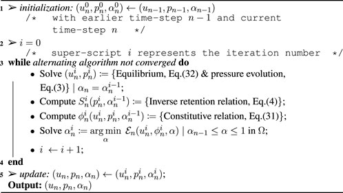
Algorithm 1. Alternating algorithm for the capillary damage model

4 Two-Dimensional Desiccation Problem

The abovementioned modeling approach is now applied to study the desiccation of soils. As already mentioned in the Introduction, this test case comes from the various desiccation experiments that can be found in the literature, Peron et al. (2009); Shin and Santamarina (2010, 2011); Stirling (2014) to name a few. Typical desiccation experiments are carried out by subjecting a certain mass of fully saturated soil to air-drying under controlled temperature and relative humidity. For numerical purposes, the flux on the drying face/s is estimated (Stirling, 2014) using the discharge rate that is calculated from experimental measurements of mass loss of water.

Furthermore, we consider a plane-strain assumption owing to the transverse dimension of the samples in all the experiments being larger than the vertical depth. This assumption does not drastically affect the aforementioned developments. Specifically, the in-plane stress components can still be obtained from the relation Eq. 33 with the definition of stiffness tensor in index notation,

${\mathbb{C}}_{\mathit{ijkl}}^0=\lambda {\delta }_{ij}{\delta }_{kl}+\mu \left({\delta }_{ik}{\delta }_{jl}+{\delta }_{il}{\delta }_{jk}\right),i,j,k,l\in \left\{\mathrm{1,2}\right\}.(38)$

λ and μ are, respectively, the first and second Lamé parameters that are related to Young’s modulus, E, and Poisson’s ratio, ν, of the empty porous skeleton. So, the boundary value problem formed by the coupled system of equations Eq. 3, Eq. 32, and the bound-constrained minimization with respect to α, Eq. 37, are resolved with appropriately defined boundary and initial conditions as laid out further in Section 4.1 and following the algorithm described in Algorithm 1. The material properties of the porous medium and the parameters of the model chosen for the purpose of the simulations are listed in Table 1, which are in the range typical of silica sands saturated with an air–water mixture.

TABLE 1

TABLE 1. Material properties and model parameters used throughout the article unless mentioned otherwise.

During the experiments in the aforementioned literature, two stages were observed in the drying process. The first stage involves large irreversible deformations with the degree of saturation close to 1 and the second stage involves a noticeable decrease in the saturation degree and with smaller deformations. Fracture initiation usually was associated with the sample close to full saturation and the air–water interface coinciding with the apparent soil surface. In the current modeling context, damage initiation is associated with the threshold, w₁, appearing within the local dissipation contribution, Eq. 11, to the bulk energy density and this, as mentioned earlier, is understood as not directly related to fracture toughness of the material but to the creation of a new fluid–fluid interface within the porous medium. Nevertheless, w₁ is a parameter that depends on the material and boundary conditions. For instance, Holtzman et al. (2012) have shown experimentally that fracturing is the preferred mode of invasion of air into water-saturated granular media when the confining stress is lower. So, this threshold can only be characterized through experimental observation of fracture initiation, viewed as a localization of the damage variable within the model. For the purpose of the current investigation, various values of w₁ are tested that either initiate damage or not, and in the former case, the possibility of localization is studied.

4.1 Problem Setup

The reference initial configuration is a rectangular domain Ω = (0, L) × (0, H) as shown in the Figure 2 with the boundary ∂Ω = {(x₁ = 0) ∪ (x₁ = L) ∪ (x₂ = 0) ∪ (x₂ = H)}. At time t = 0, it is assumed that the porous solid is completely intact, stress-free, and fully saturated giving,

${\alpha }_0\left(x\right)=0,u_0\left(x\right)=0,{\epsilon }_0\left(x\right)=0,S_0\left(x\right)=1,p_0\left(x\right)=0.(39)$

x ∈ Ω is the position vector given by x = x₁e₁ + x₂e₂. The horizontal and vertical displacements are set to vanish, respectively, on the lateral (x₁ = 0, x₁ = L) and the bottom (x₂ = H) faces along with the shear stresses at those boundaries. The top face at x₂ = 0 is a free surface. These set of mechanical boundary conditions ∀t ≥ 0 read,

$\begin{array}{ll}\hfill u_t\cdot \left(-e_1\right){|\left.\right|}_{\left(x_1=0\right)}& =0,u_t\cdot e_1|{}_{\left(x_1=L\right)}=0,u_t\cdot e_2|{}_{\left(x_2=H\right)}=0,\hfill \\ \hfill e_2\cdot {\sigma }_t\cdot \left(-e_1\right)|{}_{\left(x_1=0\right)}& =0,e_2\cdot {\sigma }_t\cdot e_1|{}_{\left(x_1=L\right)}=0,\hfill \\ \hfill {\sigma }_t\cdot \left(-e_2\right)|{}_{\left(x_2=0\right)}& =0,e_1\cdot {\sigma }_t\cdot e_2|{}_{\left(x_2=H\right)}=0.\hfill \end{array}(40)$

FIGURE 2

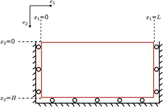
FIGURE 2. Reference configuration of the desiccation problem.

Damage is not prescribed and is free to evolve at all the boundaries whenever the damage criterion is met. Accordingly, the natural boundary condition on damage reads,

$\frac{\partial {\alpha }_t}{\partial \widehat{n}}|{\left.\right|}_{x\in \partial \mathrm{\Omega }}=0\forall t\ge 0.(41)$

For the hydraulic problem, the lateral and bottom faces are set to be impermeable. The loading is carried out by a constant imposed outward flux, − q_fe₂, on the top face, thus inducing a drying effect. While the drying flux measured using the discharge rates in Stirling (2014) is found to be a function of time, we choose to make a simplifying assumption of constant flux. These boundary conditions ∀t ≥ 0 read,

$\begin{array}{ll}\hfill \nabla p_t\cdot \left(-e_1\right)|{\left.\right|}_{\left(x_1=0\right)}& =0,\nabla p_t\cdot e_1|{\left.\right|}_{\left(x_1=L\right)}=0,\hfill \\ \hfill \left(-\frac{\varkappa }{{\eta }_w}{K}_{rw}\left(p_t\right)\nabla p_t\right)\cdot \left(-e_2\right)|{\left.\right|}_{\left(x_2=0\right)}& =q_f,\nabla p_t\cdot e_2|{\left.\right|}_{\left(x_2=H\right)}=0.\hfill \end{array}(42)$

4.2 One-Dimensional Base Solutions

It can be seen from the problem setup that the geometry, material properties, and initial conditions are invariant along the x₁-direction. The loading and boundary conditions on the top and bottom faces are as well-invariant along the x₁-direction. The boundary conditions on the lateral faces demand vanishing gradients of the solution along the x₁-direction. So, even though the problem does not render itself for obtaining an easy exact solution due to its nonlinearity, one can a priori anticipate the existence of a particular class of solutions that are homogeneous in the x₁-direction and are dependent only on x₂. Such solutions are termed here as base solutions. In fact, to obtain the base solutions, one just needs to solve the problem in one-dimension along the x₂-direction with appropriate boundary conditions, instead of the full two-dimensional problem posed earlier. This is the purpose that is explained in this section. Rigorous mathematical proof of the existence and uniqueness of such base solutions for all times is out of the scope of the current work. Instead, we exhibit numerically these solutions for t > 0.

The domain of the one-dimensional problem is defined $\tilde{\mathrm{\Omega }}=(0,H)$ along the x₂-coordinate, with boundary $\partial \tilde{\mathrm{\Omega }}=\{(x_2=0)\cup (x_2=H)\}$. The initial and boundary conditions from Section 4.1 are adapted to this domain. While studying the influence of depth H could be interesting, we choose a depth such that H ≫ ℓ.

In view of the damage criterion, Eq. 30, with the definition of average pore-pressure, $p_t^{\ast }(S_t,{\alpha }_t)=p_t(S_t,{\alpha }_t)S_t$, the solution states can be classified into two: undamaged $({\alpha }_t=0\forall x_2\in \tilde{\mathrm{\Omega }})$ and damaged $(\exists x_2\in \tilde{\mathrm{\Omega }}\mid {\alpha }_t>0)$. Since the initial state at t = 0 is assumed to be that of a uniformly intact solid, damage would initiate if the following local damage criterion is an equality.

${\varphi }_t{U}^{\prime }\left({\alpha }_t;S_t\right)-p_t^{\prime }{S}_t{\varphi }_t+w^{\prime }\left({\alpha }_t\right)\ge 0\text{\hspace{0.17em}in\hspace{0.17em}}\tilde{\mathrm{\Omega }},(43)$

where Eq. 1 gives $-p_t^{\prime }=p_c^{\prime }(S_t,{\alpha }_t)=a^{\prime }({\alpha }_t){\tilde{p}}_c(S_t)$ and Eq. 7 gives $U^{\prime }({\alpha }_t;S_t)=a^{\prime }({\alpha }_t)\tilde{U}(S_t)$. In Eq. 43, the terms that drive the damage evolution are first and second. Now for α_t = 0, a′(α_t) = −2, and for 0 < S_t < 1, $\tilde{U}(S_t)>0$ and ${\tilde{p}}_c(S_t)>0$. Since ${\varphi }_t\in \mathcal{P}$, the first driving term is negative, whose magnitude increases with decreasing S_t and conversely with increasing α_t. With a similar reasoning also, the second term is negative. The third term is a positive constant, w′(α_t) = w₁, acting as the threshold for damage initiation. Owing to the drying flux applied at x₂ = 0, the saturation degree is the lowest here. Thus, one can anticipate that starting from a uniformly undamaged state, the damage initiates at x₂ = 0 within a finite depth and propagates into the domain driven by desaturation. However, at initial times, since a minimum amount of capillary energy needs to be stored before damage initiation according to Eq. 43, the saturation degree everywhere in the domain could be such that the damage criterion is a strict inequality and damage does not initiate at all. So, one can envisage a finite time t_d > 0 beyond which the damage criterion is an equality at the drying boundary and so damage initiates. All the solution states for t ≥ t_d are called the damaged states, and this t_d depends on the intensity of the drying flux for a given material.

Figures 3, 4 show the time evolution of the solution and functions of the solution, with H = 1.0m, q_f = 10m.s⁻¹, and w₁ = 1000N.m⁻³. The material properties correspond to sand and the fluid combination to air–water. It can be seen that initially, damage does not evolve anywhere in the domain even though flux-induced desaturation initiates at x₂ = 0 and progresses into the domain. During this stage of evolution, the strain remains compressive and the porosity reduces from the initial value as expected within the unsaturated zone. However, once the damage criterion becomes equality, damage initiates at x₂ = 0. With damage growing from 0, the saturation degree degrades close to 0, indicating invasion of the air phase while the pore-water pressure only reduces slightly in magnitude. The paths followed by the solutions for different thresholds, w₁, in the space (S_t, p_t) are shown in Figure 5. It is clear that the path followed during the initial damage evolution is that of a ‘softening’ with respect to pore-water pressure. It is also interesting to observe that even though the drying flux at the boundary continues to drive the desaturation process, the damage stagnates at a maximum value at larger times, and this is replicated also within the domain, thus creating a zone of uniform damage. This is due to the simultaneous reduction in the magnitude of the first driving term in Eq. 43 with increasing damage so that after a certain value of damage, the criterion does not become an equality anymore, even though desaturation progresses.

FIGURE 3

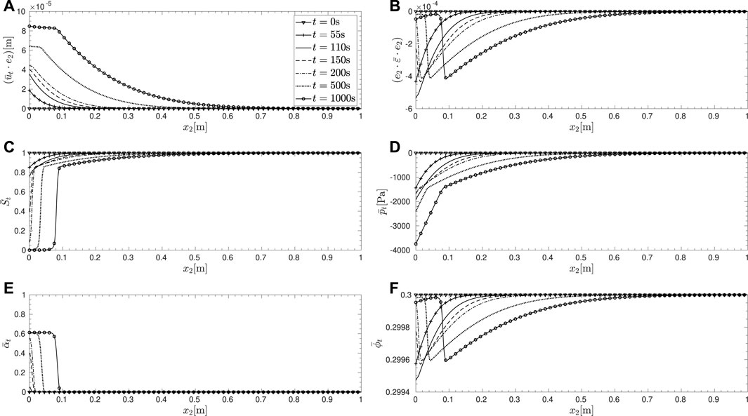
FIGURE 3. Evolution of the one-dimensional base solution and functions of the solution within the full computational domain, $\tilde{\mathrm{\Omega }}=(\mathrm{0,1}\text{m})$, for w₁ = 1000N.m⁻³.

FIGURE 4

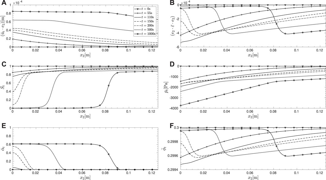
FIGURE 4. Evolution in Figure 3 shown within a restricted computational domain, $\tilde{\mathrm{\Omega }}=(\mathrm{0,0.05}\text{m})$, close to the drying boundary for clarity.

FIGURE 5

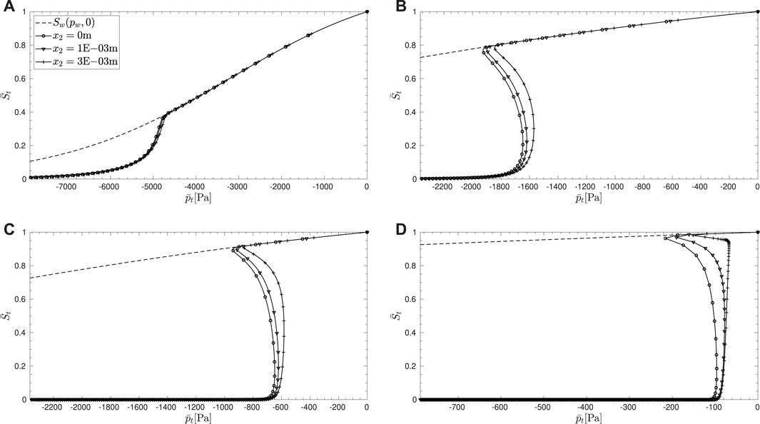
FIGURE 5. Path followed by the solution in the space (S_t, p_t) at the boundary x₂ = 0m and two locations within the domain close to this boundary for values of w₁ (A) 2000 N.m⁻³ (B) 1000 N.m⁻³, (C) 500 N.m⁻³, and (D) 100 N.m⁻³. The dashed line represents the standard non-degraded retention curve.

Figure 6 shows the time evolution of damage for different thresholds, w₁. In all cases, the damage initiates at x₂ = 0 as anticipated and then propagates into the domain supported by a finite depth, d_t, that increases with time. Lower thresholds are characterized by earlier initiation of damage and a damage value closer to 1 at the drying boundary.

FIGURE 6

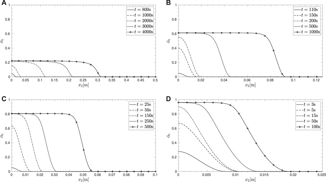
FIGURE 6. Evolution of damage for values of w₁ (A) 2000 N.m⁻³, (B) 1000 N.m⁻³, (C) 500 N.m⁻³, and (D) 100 N.m⁻³.

4.3 Bifurcation From and Instability of the Fundamental Branch

The one-dimensional base solutions resolved in Section 4.2 are the x₁-homogeneous solutions or the so-called fundamental states of the corresponding two-dimensional problem. These solutions are denoted by $({\bar{u}}_t,{\bar{\varphi }}_t,{\bar{\alpha }}_t)$ at time $t$ and, for consistency, the solution of the hydraulic problem by $({\bar{S}}_t,{\bar{p}}_t)$. The branch of the evolution along which all the states remain x₁-homogeneous is called the fundamental branch. Following the works of Benallal and Marigo (2006); Pham et al. (2011b); Sicsic et al. (2014) for standard gradient damage models, we investigate the possibility of bifurcation from the fundamental branch of evolution. A bifurcation in this sense is understood as the availability of admissible solution state/s other than the fundamental one. Whether or not the solution shifts from the fundamental branch depends on the loss of stability of the fundamental state itself and the characteristics of the perturbation that can cause such a shift. In the earlier mentioned works concerning standard gradient damage models, the possibility of bifurcations was associated with a loss of uniqueness criterion of the fundamental state. We follow a similar approach by first analyzing the loss of stability of the fundamental state and then the possibility of bifurcation.

4.3.1 Loss of Stability

By construction of the fundamental state, $({\bar{u}}_t,{\bar{\varphi }}_t,{\bar{\alpha }}_t)$ satisfies the first-order stability, Eq. 23. The question is if it satisfies the full stability condition. To verify this, one needs to analyze the condition Eq. 19 that is obtained by the expanding the perturbed state of energy in the vicinity of the one associated with the fundamental state,

$h{\mathcal{E}}_t^{\prime }\left({\bar{u}}_t,{\bar{\varphi }}_t,{\bar{\alpha }}_t\right)\left(v-{\bar{u}}_t,\phi -{\bar{\varphi }}_t,\beta -{\bar{\alpha }}_t\right)+\frac{h^2}{2}{\mathcal{E}}_t^{″}\left({\bar{u}}_t,{\bar{\varphi }}_t,{\bar{\alpha }}_t\right){\left(v-{\bar{u}}_t,\phi -{\bar{\varphi }}_t,\beta -{\bar{\alpha }}_t\right)}^2+o\left(h^2\right)\ge 0.(44)$

By virtue of the equilibrium, Eq. 24, and zeroth-order balance, Eq. 26, the FDD in Eq. 44 reduces to,

$\begin{array}{ll}\hfill {\mathcal{E}}_t^{\prime }\left({\bar{u}}_t,{\bar{\varphi }}_t,{\bar{\alpha }}_t\right)\left(v-{\bar{u}}_t,\phi -{\bar{\varphi }}_t,\beta -{\bar{\alpha }}_t\right)& =\underset{\mathrm{\Omega }}{\int }\left\{\left(-{\pi }_t^{\prime }{\bar{\varphi }}_t+w^{\prime }\left({\bar{\alpha }}_t\right)\right)\times \left(\beta -{\bar{\alpha }}_t\right)\right.\left.+w_1{\ell }^2\nabla {\bar{\alpha }}_t\cdot \nabla \left(\beta -{\bar{\alpha }}_t\right)\right\}dx,\hfill \end{array}(45)$

with the directions $(v-{\bar{u}}_t,\phi -{\bar{\varphi }}_t,\beta -{\bar{\alpha }}_t)\in \mathcal{C}\times \widehat{\mathcal{P}}\times {\widehat{\mathcal{D}}}_t^d$, with $\widehat{\mathcal{P}}$ defined in Eq. 22 and

${\widehat{\mathcal{D}}}_t^d=\left\{\widehat{\beta }\in H^1\left(\mathrm{\Omega }\right):0\le \widehat{\beta }<1\text{in}{\mathrm{\Omega }}_t^d\widehat{\beta }=0\text{in}{\mathrm{\Omega }}_t^e\right\},(46)$

where ${\mathrm{\Omega }}_t^d=(0,L)\times (0,d_t)$ is the damaged strip if damage initiates and ${\mathrm{\Omega }}_t^e=\mathrm{\Omega }\backslash {\mathrm{\Omega }}_t^d$ is the undamaged region.

Undamaged States:

For t < t_d, ${\bar{\alpha }}_t=0$ throughout Ω and the FDD is positive for all directions $(v-{\bar{u}}_t,\phi -{\bar{\varphi }}_t,\beta )$ if β ≠ 0. For directions such that $\beta ={\bar{\alpha }}_t=0$, the FDD vanishes and the SDD, Eq. 21, reduces to,

${\mathcal{E}}_t^{″}\left({\bar{u}}_t,{\bar{\varphi }}_t,{\bar{\alpha }}_t\right){\left(v-{\bar{u}}_t,\phi -{\bar{\varphi }}_t,\beta -{\bar{\alpha }}_t\right)}^2=\underset{\mathrm{\Omega }}{\int }\left\{{\mathbb{C}}^0\epsilon (v-{\bar{u}}_t)\cdot \epsilon (v-{\bar{u}}_t)+N{\left(bϵ(v-{\bar{u}}_t)-(\phi -{\bar{\varphi }}_t)\right)}^2\right\}dx,(47)$

which is positive. Hence, full stability of the fundamental state is guaranteed for t < t_d.

Damaged States:

For t ≥ t_d, the damage criterion is an equality within the damaged strip ${\mathrm{\Omega }}_t^d=(0,L)\times (0,d_t)$ and an inequality everywhere else, ${\mathrm{\Omega }}_t^e=\mathrm{\Omega }\backslash {\mathrm{\Omega }}_t^d$. If we consider directions such that $\beta \ne {\bar{\alpha }}_t$, then the FDD is positive within ${\mathrm{\Omega }}_t^e$ owing to the strict inequality of the local damage criterion, whereas a vanishing FDD corresponds to directions such that $\beta ={\bar{\alpha }}_t=0$ in ${\mathrm{\Omega }}_t^e$. In such directions, stability of the fundamental state is guaranteed if,

${\mathcal{E}}_t^{″}\left({\bar{u}}_t,{\bar{\varphi }}_t,{\bar{\alpha }}_t\right){\left(v-{\bar{u}}_t,\phi -{\bar{\varphi }}_t,\beta -{\bar{\alpha }}_t\right)}^2>0,\forall \left(v,\phi ,\beta \right)\in \mathcal{C}\times \mathcal{P}\times {\mathcal{D}}_t^d,(48)$

and only if the above inequality is not strict. It should be noted that in the abovementioned equation, the expression of SDD is given by Eq. 21 and not by the reduced Eq. 47 owing to the possibility of $\beta \ne {\bar{\alpha }}_t$ in ${\mathrm{\Omega }}_t^d$. ${\mathcal{D}}_t^d\subset {\mathcal{D}}_t$, is the set of admissible damage fields given by,

${\mathcal{D}}_t^d=\left\{\beta \in H^1\left(\mathrm{\Omega }\right):{\bar{\alpha }}_t\le \beta <1\text{in}{\mathrm{\Omega }}_t^d,\beta =0\text{in}{\mathrm{\Omega }}_t^e\right\}.(49)$

The directions $(v-{\bar{u}}_t,\phi -{\bar{\varphi }}_t,\beta -{\bar{\alpha }}_t)$ are further denoted as $(\widehat{v},\widehat{\phi },\widehat{\beta })\in \mathcal{C}\times \widehat{\mathcal{P}}\times {\widehat{\mathcal{D}}}_t^d$, with an abuse of notation w.r.t the notation introduced in Section 2.3.

Noting, for the moment, that SDD in the damaged states is evaluated at the fundamental state and analysis of the condition in Eq. 48 is deferred to a later moment in view of studying the possibility of bifurcations.

Synopsis: While the undamaged states are fully stable, the damaged states are conditionally stable and this condition amounts to verifying the positive definiteness of the quadratic form ${\mathcal{E}}_t^{″}({\bar{u}}_t,{\bar{\varphi }}_t,{\bar{\alpha }}_t){(\cdot )}^2$ when applied on directions belonging to $\mathcal{C}\times \dot{\mathcal{P}}\times {\dot{\mathcal{D}}}_t^d$. Specifically,

$\forall \left(\widehat{v},\widehat{\phi },\widehat{\beta }\right)\in \mathcal{C}\times \widehat{\mathcal{P}}\times {\widehat{\mathcal{D}}}_t^d\left\{\begin{array}{c}{\mathcal{E}}_t^{″}\left({\bar{u}}_t,{\bar{\varphi }}_t,{\bar{\alpha }}_t\right){\left(\widehat{v},\widehat{\phi },\widehat{\beta }\right)}^2>0\Rightarrow \mathit{\text{stability}}\hfill \\ {\mathcal{E}}_t^{″}\left({\bar{u}}_t,{\bar{\varphi }}_t,{\bar{\alpha }}_t\right){\left(\widehat{v},\widehat{\phi },\widehat{\beta }\right)}^2<0\Rightarrow \mathit{\text{instability}}.\hfill \end{array}\right.(50)$

4.3.2 Possibility of Bifurcations

As mentioned earlier, the notion of bifurcation from the fundamental branch is intertwined with the availability of admissible solution state/s other than the fundamental one. This amounts to studying the evolution problem at time t + η, with η > 0 small enough, knowing that the solution has followed the fundamental branch up until t, that is, knowing the solution at t is $({\bar{u}}_t,{\bar{\varphi }}_t,{\bar{\alpha }}_t)$. Before proceeding further, we assume that such an evolution is smooth enough that forward time derivatives of the solution components exist at time t and are defined

$\dot{u}=\underset{\eta \to 0}{\lim }\frac{u_{t+\eta }-{\bar{u}}_t}{\eta },\dot{\varphi }=\underset{\eta \to 0}{\lim }\frac{{\varphi }_{t+\eta }-{\bar{\varphi }}_t}{\eta },\dot{\alpha }=\underset{\eta \to 0}{\lim }\frac{{\alpha }_{t+\eta }-{\bar{\alpha }}_t}{\eta }.(51)$

Furthermore, a smooth growth of the damage zone is assumed within the time interval (t, t + η). More detail of such a hypothesis can be found in Sicsic et al. (2014). Now, if the solution continues to stay on the fundamental branch, then it implies that $(\dot{u},\dot{\varphi },\dot{\alpha })$ are as well x₁-homogeneous giving, $(\dot{u},\dot{\varphi },\dot{\alpha })=(\dot{\stackrel{̄}{u}},\dot{\stackrel{̄}{\varphi }},\dot{\stackrel{̄}{\alpha }})$. However, if bifurcation is to happen, then there should be some other solution rate $(\dot{u},\dot{\varphi },\dot{\alpha })$. To check this possibility we derive from the evolution problem at t + η, a rate problem that any solution rate needs to satisfy.

Imposing (u_t+η, ϕ_t+η, α_t+η) to satisfy the three evolution principles in Section 2.2, we get:

1) Irreversibility of damage: Damage must be nondecreasing, that is, $\dot{\alpha }\ge 0$. Consequently, $(\dot{u},\dot{\varphi },\dot{\alpha })\in \mathcal{C}\times \dot{\mathcal{P}}\times \dot{\mathcal{D}}$, with,

$\dot{\mathcal{P}}=\left\{\phi \in H^1\left(\mathrm{\Omega }\right)\right\},\dot{\mathcal{D}}=\left\{\beta \in H^1\left(\mathrm{\Omega }\right):\beta \ge 0\text{in}\mathrm{\Omega }\right\}.(52)$

2) Stability: Directional stability implies first-order stability which at (u_t+η, ϕ_t+η, α_t+η) reads,

${\mathcal{E}}_{t+\eta }^{\prime }\left(u_{t+\eta },{\varphi }_{t+\eta },{\alpha }_{t+\eta }\right)\left(\widehat{v},\widehat{\phi },\widehat{\beta }\right)\ge 0\forall \left(\widehat{v},\widehat{\phi },\widehat{\beta }\right)\in \mathcal{C}\times \widehat{\mathcal{P}}\times \mathcal{D}.(53)$

As analyzed earlier for loss of stability of the fundamental state at time t, for directions $(\widehat{v},\widehat{\phi },\widehat{\beta })$ such that ${\mathcal{E}}_t^{\prime }({\bar{u}}_t,{\bar{\varphi }}_t,{\bar{\alpha }}_t)(\widehat{v},\widehat{\phi },\widehat{\beta })>0$, by continuity, Eq. 53 and consequently full stability of the state (u_t+η, ϕ_t+η, α_t+η) hold true.

Whereas for directions such that ${\mathcal{E}}_t^{\prime }({\bar{u}}_t,{\bar{\varphi }}_t,{\bar{\alpha }}_t)(\widehat{v},\widehat{\phi },\widehat{\beta })=0$, this is not evident. In fact, such directions correspond to $\widehat{\beta }=0$ in ${\mathrm{\Omega }}_t^e$, that is, $\widehat{\beta }\in {\widehat{\mathcal{D}}}_t^d$. Dividing Eq. 53 by η and passing to the limit when η tends to 0 gives the following condition on any $(\dot{u},\dot{\varphi },\dot{\alpha })\in \mathcal{C}\times \dot{\mathcal{P}}\times {\dot{\mathcal{D}}}_t^d$,

$\begin{array}{ll}\hfill {\mathcal{E}}_t^{″}\left({\bar{u}}_t,{\bar{\varphi }}_t,{\bar{\alpha }}_t\right)⟨\left(\dot{u},\dot{\varphi },\dot{\alpha }\right),\left(\widehat{v},\widehat{\phi },\widehat{\beta }\right)⟩+& {\dot{\mathcal{E}}}_t^{\prime }\left({\bar{u}}_t,{\bar{\varphi }}_t,{\bar{\alpha }}_t\right)\left(\widehat{v},\widehat{\phi },\widehat{\beta }\right)\ge 0\hfill \\ \hfill & \forall \left(\widehat{v},\widehat{\phi },\widehat{\beta }\right)\in \mathcal{C}\times \widehat{\mathcal{P}}\times {\widehat{\mathcal{D}}}_t^d,\hfill \end{array}(54)$

with¹,

${\dot{\mathcal{D}}}_t^d=\left\{\beta \in H^1\left(\mathrm{\Omega }\right):\beta \ge 0\text{in}{\mathrm{\Omega }}_t^d,\beta =0\text{in}{\mathrm{\Omega }}_t^e\right\}.(55)$

3) Energy Balance: The energy balance at time t + η reads,

${\mathcal{E}}_{t+\eta }\left(u_{t+\eta },{\varphi }_{t+\eta },{\alpha }_{t+\eta }\right)={\mathcal{E}}_t\left({\bar{u}}_t,{\bar{\varphi }}_t,{\bar{\alpha }}_t\right)-\underset{t}{\overset{t+h}{\int }}\underset{\mathrm{\Omega }}{\int }\left(\frac{\partial {\pi }_s}{\partial S_s}{\varphi }_s\right){\dot{S}}_{s}dxds.(56)$

A first expansion of ${\mathcal{E}}_{t+\eta }(u_{t+\eta },{\varphi }_{t+\eta },{\alpha }_{t+\eta })$ on the left-hand side of the above equation up to second-order leads to,

$\begin{array}{ll}\hfill & {\mathcal{E}}_{t+\eta }\left({\bar{u}}_t,{\bar{\varphi }}_t,{\bar{\alpha }}_t\right)+{\mathcal{E}}_{t+\eta }^{\prime }\left({\bar{u}}_t,{\bar{\varphi }}_t,{\bar{\alpha }}_t\right)\left(u_{t+\eta }-{\bar{u}}_t,{\varphi }_{t+\eta }-{\bar{\varphi }}_t,{\alpha }_{t+\eta }-{\bar{\alpha }}_t\right)\hfill \\ \hfill & +\frac{1}{2}{\mathcal{E}}_{t+\eta }^{″}\left({\bar{u}}_t,{\bar{\varphi }}_t,{\bar{\alpha }}_t\right){\left(u_{t+\eta }-{\bar{u}}_t,{\varphi }_{t+\eta }-{\bar{\varphi }}_t,{\alpha }_{t+\eta }-{\bar{\alpha }}_t\right)}^2\hfill \\ \hfill & +o\left(\Vert \left(u_{t+\eta }-{\bar{u}}_t,{\varphi }_{t+\eta }-{\bar{\varphi }}_t,{\alpha }_{t+\eta }-{\bar{\alpha }}_t\right){\Vert }^2\right)\hfill \\ \hfill & ={\mathcal{E}}_t\left({\bar{u}}_t,{\bar{\varphi }}_t,{\bar{\alpha }}_t\right)-\underset{t}{\overset{t+h}{\int }}\underset{\mathrm{\Omega }}{\int }\left(\frac{\partial {\pi }_s}{\partial S_s}{\varphi }_s\right){\dot{S}}_{s}dxds,\hfill \end{array}(57)$

where ‖ ⋅‖ denotes the norm of $\mathcal{C}\times \widehat{\mathcal{P}}\times \mathcal{D}$. A second expansion in time up to second-order of the operators at t + η leads to,

$\begin{array}{ll}\hfill {\mathcal{E}}_t^{\prime }\left({\bar{u}}_t,{\bar{\varphi }}_t,{\bar{\alpha }}_t\right)\left(u_{t+\eta }-{\bar{u}}_t,{\varphi }_{t+\eta }-{\bar{\varphi }}_t,{\alpha }_{t+\eta }-{\bar{\alpha }}_t\right)& +{\eta }^2{\dot{\mathcal{E}}}_t^{\prime }\left({\bar{u}}_t,{\bar{\varphi }}_t,{\bar{\alpha }}_t\right)\left(\dot{u},\dot{\varphi },\dot{\alpha }\right)\hfill \\ \hfill & +\frac{{\eta }^2}{2}{\mathcal{E}}_t^{″}\left({\bar{u}}_t,{\bar{\varphi }}_t,{\bar{\alpha }}_t\right){\left(\dot{u},\dot{\varphi },\dot{\alpha }\right)}^2\hfill \\ \hfill & +\eta {\dot{\mathcal{E}}}_t\left({\bar{u}}_t,{\bar{\varphi }}_t,{\bar{\alpha }}_t\right)+\frac{{\eta }^2}{2}{\ddot{\mathcal{E}}}_t\left({\bar{u}}_t,{\bar{\varphi }}_t,{\bar{\alpha }}_t\right)+o\left({\eta }^2\right)\hfill \\ \hfill & =-\eta \underset{\mathrm{\Omega }}{\int }\left(\frac{\partial {\pi }_t}{\partial S_t}{\bar{\varphi }}_t\right){\dot{S}}_{t}dx-\frac{{\eta }^2}{2}\frac{d}{dt}\left(\underset{\mathrm{\Omega }}{\int }\left(\frac{\partial {\pi }_t}{\partial S_t}{\bar{\varphi }}_t\right){\dot{S}}_{t}dx\right).\hfill \end{array}(58)$

The following definitions are obtained by differentiating with respect to time the energy balance written at time t,

$\begin{array}{ll}\hfill {\dot{\mathcal{E}}}_t\left({\bar{u}}_t,{\bar{\varphi }}_t,{\bar{\alpha }}_t\right)& =-\underset{\mathrm{\Omega }}{\int }\left(\frac{\partial {\pi }_t}{\partial S_t}{\bar{\varphi }}_t\right){\dot{S}}_{t}dx,{\ddot{\mathcal{E}}}_t\left({\bar{u}}_t,{\bar{\varphi }}_t,{\bar{\alpha }}_t\right)\hfill \\ \hfill & =-\frac{d}{dt}\left(\underset{\mathrm{\Omega }}{\int }\left(\frac{\partial {\pi }_t}{\partial S_t}{\bar{\varphi }}_t\right){\dot{S}}_{t}dx\right).\hfill \end{array}(59)$

The term ${\mathcal{E}}_t^{\prime }({\bar{u}}_t,{\bar{\varphi }}_t,{\bar{\alpha }}_t)(u_{t+\eta }-{\bar{u}}_t,{\varphi }_{t+\eta }-{\bar{\varphi }}_t,{\alpha }_{t+\eta }-{\bar{\alpha }}_t)$ is o(η²) due to the assumption of smooth growth of the damage zone and $\dot{\alpha }\in {\mathcal{D}}_t^d$; see Sicsic et al. (2014) for a detailed deduction. So, one obtains by diving Eq. 58 by η² and passing to the limit when η tends to be 0,

${\dot{\mathcal{E}}}_t^{\prime }\left({\bar{u}}_t,{\bar{\varphi }}_t,{\bar{\alpha }}_t\right)\left(\dot{u},\dot{\varphi },\dot{\alpha }\right)+{\mathcal{E}}_t^{″}\left({\bar{u}}_t,{\bar{\varphi }}_t,{\bar{\alpha }}_t\right){\left(\dot{u},\dot{\varphi },\dot{\alpha }\right)}^2=0.(60)$

The rate problem: Subtracting Eq. 60 from Eq. 54 gives the following inequality that the rate at any time t > 0, $(\dot{u},\dot{\varphi },\dot{\alpha })\in \mathcal{C}\times \dot{\mathcal{P}}\times {\dot{\mathcal{D}}}_t^d$, needs to satisfy,

$\begin{array}{ll}\hfill {\mathcal{E}}_t^{″}\left({\bar{u}}_t,{\bar{\varphi }}_t,{\bar{\alpha }}_t\right)⟨\left(\dot{u},\dot{\varphi },\dot{\alpha }\right),\left(\widehat{v}-\dot{u},\widehat{\phi }-\dot{\varphi },\widehat{\beta }-\dot{\alpha }\right)⟩& +{\dot{\mathcal{E}}}_t^{\prime }\left({\bar{u}}_t,{\bar{\varphi }}_t,{\bar{\alpha }}_t\right)\left(\widehat{v}-\dot{u},\widehat{\phi }-\dot{\varphi },\widehat{\beta }-\dot{\alpha }\right)\ge 0\hfill \\ \hfill \forall \left(\widehat{v},\widehat{\phi },\widehat{\beta }\right)\in \mathcal{C}\times \widehat{\mathcal{P}}& \times {\widehat{\mathcal{D}}}_t^d.\hfill \end{array}(61)$

To verify if any rate other than the x₁-homogeneous rate, $(\dot{\stackrel{̄}{u}},\dot{\stackrel{̄}{\varphi }},\dot{\stackrel{̄}{\alpha }})$, satisfies the rate problem we proceed as follows. First choosing $(\widehat{v},\widehat{\phi },\widehat{\beta })=(\dot{\stackrel{̄}{u}},\dot{\stackrel{̄}{\varphi }},\dot{\stackrel{̄}{\alpha }})$ in Eq. 61, we get,

${\mathcal{E}}_t^{″}\left({\bar{u}}_t,{\bar{\varphi }}_t,{\bar{\alpha }}_t\right)⟨\left(\dot{u},\dot{\varphi },\dot{\alpha }\right),\left(\dot{\stackrel{̄}{u}}-\dot{u},\dot{\stackrel{̄}{\varphi }}-\dot{\varphi },\dot{\stackrel{̄}{\alpha }}-\dot{\alpha }\right)⟩+{\dot{\mathcal{E}}}_t^{\prime }\left({\bar{u}}_t,{\bar{\varphi }}_t,{\bar{\alpha }}_t\right)\left(\dot{\stackrel{̄}{u}}-\dot{u},\dot{\stackrel{̄}{\varphi }}-\dot{\varphi },\dot{\stackrel{̄}{\alpha }}-\dot{\alpha }\right)\ge 0.(62)$

Whereas by choosing $(\widehat{v},\widehat{\phi },\widehat{\beta })=(\dot{u},\dot{\varphi },\dot{\alpha })$ in Eq. 61 that is already written with $(\dot{\stackrel{̄}{u}},\dot{\stackrel{̄}{\varphi }},\dot{\stackrel{̄}{\alpha }})$ as the solution, we get,

${\mathcal{E}}_t^{″}\left({\bar{u}}_t,{\bar{\varphi }}_t,{\bar{\alpha }}_t\right)⟨\left(\dot{\stackrel{̄}{u}},\dot{\stackrel{̄}{\varphi }},\dot{\stackrel{̄}{\alpha }}\right),\left(\dot{u}-\dot{\stackrel{̄}{u}},\dot{\varphi }-\dot{\stackrel{̄}{\varphi }},\dot{\alpha }-\dot{\stackrel{̄}{\alpha }}\right)⟩+{\dot{\mathcal{E}}}_t^{\prime }\left({\bar{u}}_t,{\bar{\varphi }}_t,{\bar{\alpha }}_t\right)\left(\dot{u}-\dot{\stackrel{̄}{u}},\dot{\varphi }-\dot{\stackrel{̄}{\varphi }},\dot{\alpha }-\dot{\stackrel{̄}{\alpha }}\right)\ge 0.(63)$

Adding Eq. 62 and Eq. 63, we get the inequality,

${\mathcal{E}}_t^{″}\left({\bar{u}}_t,{\bar{\varphi }}_t,{\bar{\alpha }}_t\right){\left(\dot{u}-\dot{\stackrel{̄}{u}},\dot{\varphi }-\dot{\stackrel{̄}{\varphi }},\dot{\alpha }-\dot{\stackrel{̄}{\alpha }}\right)}^2\le 0.(64)$

This condition holds true only if $(\dot{u},\dot{\varphi },\dot{\alpha })=(\dot{\stackrel{̄}{u}},\dot{\stackrel{̄}{\varphi }},\dot{\stackrel{̄}{\alpha }})$, when ${\mathcal{E}}_t^{″}({\bar{u}}_t,{\bar{\varphi }}_t,{\bar{\alpha }}_t)$ is positive definite, thus indicating a uniqueness criterion for the solution of the rate problem. It is to be noted that both $(\dot{u},\dot{\varphi },\dot{\alpha })$ and $(\dot{\stackrel{̄}{u}},\dot{\stackrel{̄}{\varphi }},\dot{\stackrel{̄}{\alpha }})$ come from the same space, whereas $(\dot{u}-\dot{\stackrel{̄}{u}},\dot{\varphi }-\dot{\stackrel{̄}{\varphi }},\dot{\alpha }-\dot{\stackrel{̄}{\alpha }})\in \mathcal{C}\times \dot{\mathcal{P}}\times {\dot{\mathcal{D}}}_t$ where ${\dot{\mathcal{D}}}_t$ is the linear space associated with ${\widehat{\mathcal{D}}}_t^d$ at time t defined as,

${\dot{\mathcal{D}}}_t=\left\{\beta \in H^1\left(\mathrm{\Omega }\right):\beta =0\text{in}{\mathrm{\Omega }}_t^e\right\}.(65)$

Synopsis: The uniqueness of the x₁-homogeneous rate solution of the rate problem and consequently the impossibility of bifurcation from the fundamental branch are ensured by the positive definiteness of the quadratic form ${\mathcal{E}}_t^{″}({\bar{u}}_t,{\bar{\varphi }}_t,{\bar{\alpha }}_t){(\cdot )}^2$ when applied on directions belonging to $\mathcal{C}\times \dot{\mathcal{P}}\times {\dot{\mathcal{D}}}_t$. Specifically,

$\forall \left(\widehat{v},\widehat{\phi },\widehat{\beta }\right)\in \mathcal{C}\times \dot{\mathcal{P}}\times {\dot{\mathcal{D}}}_t\left\{\begin{array}{c}{\mathcal{E}}_t^{″}\left({\bar{u}}_t,{\bar{\varphi }}_t,{\bar{\alpha }}_t\right){\left(\widehat{v},\widehat{\phi },\widehat{\beta }\right)}^2>0\Rightarrow \mathit{\text{no bifurcation}}\hfill \\ {\mathcal{E}}_t^{″}\left({\bar{u}}_t,{\bar{\varphi }}_t,{\bar{\alpha }}_t\right){\left(\widehat{v},\widehat{\phi },\widehat{\beta }\right)}^2\le 0\Rightarrow \mathit{\text{bifurcation possible}}.\hfill \end{array}\right.(66)$

Remark: One can notice from the abovementioned results that both the loss of stability of the fundamental state and the possibility of bifurcation from it amounts to studying the positive definiteness of the same quadratic form, ${\mathcal{E}}_t^{″}({\bar{u}}_t,{\bar{\varphi }}_t,{\bar{\alpha }}_t){(\cdot )}^2$, when applied on directions belonging to different spaces: $\mathcal{C}\times \widehat{\mathcal{P}}\times {\widehat{\mathcal{D}}}_t^d$ and $\mathcal{C}\times \dot{\mathcal{P}}\times {\dot{\mathcal{D}}}_t$, respectively. If t_b and t_s are two positive times at which, respectively, bifurcation from and instability of the fundamental state first occurs, then one can prove as a consequence of $\widehat{\mathcal{P}}\subset \dot{\mathcal{P}}$ and ${\widehat{D}}_t^d\subset {\dot{\mathcal{D}}}_t$ that t_b ≤ t_s. This proof is considered to be out of the scope of the current work. However, one can find such a proof in Sicsic et al. (2014) using the minimization of ‘Rayleigh’ ratios for both cases in a thermal shock problem which has a similar structure.

4.4 Characterization of Bifurcations

Now we are in a position to study the possibility of bifurcations by assuming general forms of the directions in which the quadratic form is to be applied. To this end, let $(\widehat{v},\widehat{\phi },\widehat{\beta })\in \mathcal{C}\times \dot{\mathcal{P}}\times {\dot{\mathcal{D}}}_t$ be a general direction. Its components can be decomposed into their respective Fourier modes with characteristic wave numbers $k\in \mathbb{N}$ as follows:

$\begin{array}{cc}\hfill \widehat{v}\left(x\right)\hfill & =\sum _k{v}^k\left(x\right),v^k\left(x\right)=v_1^k\left(x_2\right)\sin \left(\frac{k\pi x_1}{L}\right)e_1+v_2^k\left(x_2\right)\cos \left(\frac{k\pi x_1}{L}\right)e_2,\hfill \\ \hfill \widehat{\phi }\left(x\right)\hfill & =\sum _k{\phi }^k\left(x\right),{\phi }^k\left(x\right)={\phi }_1^k\left(x_2\right)\cos \left(\frac{k\pi x_1}{L}\right),\hfill \\ \hfill \widehat{\beta }\left(x\right)& =\sum _k{\beta }^k\left(x\right),{\beta }^k\left(x\right)={\beta }_1^k\left(x_2\right)\cos \left(\frac{k\pi x_1}{L}\right).\hfill \end{array}(67)$

While choosing the abovementioned decomposition, the boundary conditions that apply to the admissible perturbations to the fundamental state are a priori adapted to $(\widehat{v},\widehat{\phi },\widehat{\beta })$. Specifically, since the KKT conditions, Eq. 36, demand that on any boundary where damage grows, the spatial derivative normal to it vanishes and this applies to the lateral boundaries of the damaged strip and to the drying boundary, {(x₁ = 0) ∪ (x₂ ∈ (0, d_t))} and {(x₁ = L) ∪ (x₂ ∈ (0, d_t))}, whereas in ${\mathrm{\Omega }}_t^e$ since damage is uniformly zero, its spatial derivative as well vanishes at its boundaries, {(x₁ = 0) ∪ (x₂ ∈ (d_t, H))} and {(x₁ = L) ∪ (x₂ ∈ (d_t, H))}. Consequently, for the damage rate one gets, $\partial \widehat{\beta }/\partial x_1=0$ on x₁ = 0 and x₁ = L. Similarly, using the boundary conditions on displacement imply that on x₁ = 0 and x₁ = L, ${\widehat{v}}_1=0$ uniformly implying $\partial {\widehat{v}}_1/\partial x_2=0$, and since the shear stress at this boundary vanishes, we get $\partial {\widehat{v}}_2/\partial x_1=0$. In addition to the above, the x₁ independence of the fundamental state justifies the forms assumed for $\widehat{v}$ an $\widehat{\beta }$ in Eq. 67. Consequently, the following definitions for their gradients hold for each k,

$\begin{array}{ll}\hfill \epsilon \left(v^k\right)=& v_1^k\frac{k\pi }{L}\cos \left(\frac{k\pi x_1}{L}\right)e_1\otimes e_1+\frac{d{v}_2^k}{d{x}_2}\cos \left(\frac{k\pi x_1}{L}\right)e_2\otimes e_2\hfill \\ \hfill & +\frac{1}{2}\sin \left(\frac{k\pi x_1}{L}\right)\left(\frac{d{v}_1^k}{d{x}_2}-v_2^k\frac{k\pi }{L}\right)\left(e_1\otimes e_2+e_2\otimes e_1\right),\hfill \\ \hfill \nabla {\beta }^k=& -{\beta }_1^k\frac{k\pi }{L}\sin \left(\frac{k\pi x_1}{L}\right)e_1+\frac{d{\beta }_1^k}{d{x}_2}\cos \left(\frac{k\pi x_1}{L}\right)e_2.\hfill \end{array}(68)$

Owing to the classical constitutive relation for porosity, Eq. 31, obtained by rearranging the zeroth-order balance law for variations in porosity, the abovementioned definition of ɛ(v^k) and the boundary conditions of the hydraulic problem for p_t, Eq. 42, one can justify the form assumed for $\widehat{\phi }$ in Eq. 67.

Exploiting the orthogonality among different Fourier modes allows to uncouple them and evaluate the functional ${\mathcal{E}}_t^{″}(u_t,{\varphi }_t,{\alpha }_t){(\widehat{v},\widehat{\phi },\widehat{\beta })}^2$ in Eq. 21 at $({\bar{u}}_t,{\bar{\varphi }}_t,{\bar{\alpha }}_t)$, in directions for each k separately. Following this and integrating once along x₁ gives,

$\begin{array}{ll}\hfill {\mathcal{E}}_t^{″}\left({\bar{u}}_t,{\bar{\varphi }}_t,{\bar{\alpha }}_t\right){\left(v^k,{\phi }^k,{\beta }^k\right)}^2& =\frac{L}{2}\underset{x_2=0}{\overset{x_2=H}{\int }}\left\{\lambda {\left[v_1^k\frac{k\pi }{L}+\frac{d{v}_2^k}{d{x}_2}\right]}^2+2\mu \left[{\left(v_1^k\frac{k\pi }{L}\right)}^2+{\left(\frac{d{v}_2^k}{d{x}_2}\right)}^2\right]\right.+\mu {\left[\frac{d{v}_1^k}{d{x}_2}-v_2^k\frac{k\pi }{L}\right]}^2+N{\left[b\left(v_1^k\frac{k\pi }{L}+\frac{d{v}_2^k}{d{x}_2}\right)-{\phi }_1^k\right]}^2\hfill \\ \hfill & -{\bar{\varphi }}_t{\bar{\pi }}_t^{″}{\left({\beta }_1^k\right)}^2-2{\bar{\pi }}_t^{\prime }{\phi }_1^k{\beta }_1^k+w_1{\ell }^2\left[{\left({\beta }_1^k\frac{k\pi }{L}\right)}^2+{\left(\frac{d{\beta }_1^k}{d{x}_2}\right)}^2\right]\}dx,\hfill \end{array}(69)$

where functions denoted $(\bar{\cdot })$ are to be understood as evaluated at the fundamental state. Dependency on the wave number in the abovementioned expression can be understood as a parametrization and study of the positivity of the quadratic form can be recast into a comparison with 0 the smallest eigenvalue of the eigenproblem,

$\left({\mathcal{E}}_t^{″}\left({\bar{u}}_t,{\bar{\varphi }}_t,{\bar{\alpha }}_t;k\right)-{\mu }_k\mathbb{I}\right){\left(v_1^k,v_2^k,{\phi }_1^k,{\beta }_1^k\right)}^2=0,\forall k\in \mathbb{N},(70)$

where μ_k denotes the eigenvalues and $(v_1^k,v_2^k,{\phi }_1^k,{\beta }_1^k)$ the eigenvectors for each k.

Accordingly, the criterion for bifurcation, Eq. 66, at each time t > 0 can be translated to,

$\forall k\in \mathbb{N}\forall \left(v_1^k,v_2^k,{\phi }_1^k,{\beta }_1^k\right)\in H^1\left(\tilde{\mathrm{\Omega }}\right)\times H_0^1\left(\tilde{\mathrm{\Omega }}\right)\times H^1\left(\tilde{\mathrm{\Omega }}\right)\times H_t^1\left(\tilde{\mathrm{\Omega }}\right)\left\{\begin{array}{c}\inf \left\{\mathfrak{R}\left({\mu }_k\right)\right\}>0\Rightarrow \mathit{\text{no bifurcation}}\hfill \\ \inf \left\{\mathfrak{R}\left({\mu }_k\right)\right\}\le 0\Rightarrow \mathit{\text{bifurcation possible}},\hfill \end{array}\right.(71)$

with $H_0^1(\tilde{\mathrm{\Omega }})$ being the space of H¹ functions in $\tilde{\mathrm{\Omega }}$, vanishing at x₂ = H and $H_t^1(\tilde{\mathrm{\Omega }})$ are those vanishing in the undamaged region x₂ ∈ (d_t, H).

4.4.1 Indicative Study of Bifurcations

While the true possibility of bifurcations could be understood by the criterion Eq. 71, we can investigate the behavior of the coefficients of the quadratic form ${\mathcal{E}}_t^{″}({\bar{u}}_t,{\bar{\varphi }}_t,{\bar{\alpha }}_t){(\widehat{v},\widehat{\phi },\widehat{\beta })}^2$ which gives a qualitative indication. This is the purpose of the current section. It is to be noted that while by itself this quadratic form does not merit any physical interpretation, its evaluation in Eq. 50, Eq. 66 with respect to relevant directions informs us on the stability of solutions and the possibility of bifurcations.

By virtue of Eq. 21, we can classify the various terms within the functional as follows:

${\mathcal{E}}_t^{″}\left({\bar{u}}_t,{\bar{\varphi }}_t,{\bar{\alpha }}_t\right){\left(\widehat{v},\widehat{\phi },\widehat{\beta }\right)}^2={\mathcal{A}}_t\left({\bar{u}}_t,{\bar{\varphi }}_t,{\bar{\alpha }}_t\right){\left(\widehat{v},\widehat{\phi },\widehat{\beta }\right)}^2+{\mathcal{B}}_t\left({\bar{u}}_t,{\bar{\varphi }}_t,{\bar{\alpha }}_t\right){\left(\widehat{v},\widehat{\phi },\widehat{\beta }\right)}^2,(72)$

with

$\begin{array}{ll}\hfill {\mathcal{A}}_t\left({\bar{u}}_t,{\bar{\varphi }}_t,{\bar{\alpha }}_t\right){\left(\widehat{v},\widehat{\phi },\widehat{\beta }\right)}^2=& \underset{\mathrm{\Omega }}{\int }\left\{{\mathbb{C}}^0\epsilon \left(\widehat{v}\right)\cdot \epsilon \left(\widehat{v}\right)+N{\left(bϵ\left(\widehat{v}\right)-\widehat{\phi }\right)}^2-{\bar{\varphi }}_t{\bar{\pi }}_t^{″}{\widehat{\beta }}^2\right.\left.+w_1{\ell }^2\nabla \widehat{\beta }\cdot \nabla \widehat{\beta }\right\}dx,\hfill \\ \hfill {\mathcal{B}}_t\left({\bar{u}}_t,{\bar{\varphi }}_t,{\bar{\alpha }}_t\right){\left(\widehat{v},\widehat{\phi },\widehat{\beta }\right)}^2=& -\underset{\mathrm{\Omega }}{\int }2{\bar{\pi }}_t^{\prime }\widehat{\phi }\widehat{\beta }dx.\hfill \end{array}(73)$

We can conclude that the first term, ${\mathcal{A}}_t({\bar{u}}_t,{\bar{\varphi }}_t,{\bar{\alpha }}_t){(\widehat{v},\widehat{\phi },\widehat{\beta })}^2$, is positive definite because N and w₁ are positive constants, the stiffness tensor, ${\mathbb{C}}^0$, is positive definite, ${\bar{\varphi }}_t\in \mathcal{P}$ and ${\bar{\pi }}_t^{″}=2(-{\tilde{p}}_c({\bar{S}}_t){\bar{S}}_t-U({\bar{S}}_t))<0$. Thus, this term acts to prevent any bifurcations from occurring.

The term ${\mathcal{B}}_t({\bar{u}}_t,{\bar{\varphi }}_t,{\bar{\alpha }}_t){(\widehat{v},\widehat{\phi },\widehat{\beta })}^2$ on the other hand contributes to the possibility of bifurcations. Even if the sign of the cross term in $(\widehat{\phi }\widehat{\beta })$ could only be determined by solving the eigenproblem, its coefficient, however, is positive since ${\bar{\pi }}_t^{\prime }=-2(1-{\bar{\alpha }}_t)(-{\tilde{p}}_c({\bar{S}}_t){\bar{S}}_t-\tilde{U}({\bar{S}}_t))>0$. For the sake of being conservative, this cross term is considered negative in the following analysis.

In view of the above analysis, one can study the strength of ${\mathcal{B}}_t$ by studying the strength of its coefficient as a function of time in order to understand the behavior of bifurcations, if they occur. It can be observed that this coefficient is a function of the fundamental states that were resolved in Section 4.2. Figure 7 shows the evolution of ${\bar{\pi }}_t^{\prime }$, with respect to the saturation degree for different values of the threshold w₁. As the saturation degree reduces with time during the drying process, it can be seen that this function deviates from its undamaged path as soon as damage is initiated and its magnitude tends to reduce as damage propagates into the domain. This indicates that the term ${\mathcal{B}}_t$ reduces with time, and one can infer that the tendency to bifurcate from the fundamental branch reduces as well. For higher values of w₁, however, the magnitude of ${\bar{\pi }}_t^{\prime }$ starts to pick up after the initial reduction. However, the rate of this increase was found to be extremely slow due to the saturation degree being close to vanishing and the path followed is on a very steep degraded retention curve as seen in Figure 5A. One can make similar inferences for the loss of stability as well since, as remarked earlier, it also amounts to the study of a quadratic form involving the same operator, ${\mathcal{E}}_t^{″}({\bar{u}}_t,{\bar{\varphi }}_t,{\bar{\alpha }}_t)$ according to Eq. 50.

FIGURE 7

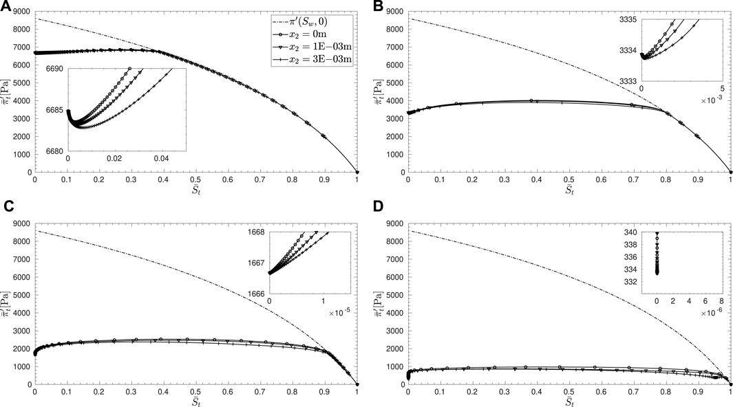
FIGURE 7. Evolution of the functions, ${\bar{\pi }}_t^{\prime },$ with S_t at the boundary x₂ = 0m and two locations within the domain close to this boundary. The different values of w₁ used are (A) 2000 N.m⁻³, (B) 1000 N.m⁻³, (C) 500 N.m⁻³, and (D) 100 N.m⁻³. In each plot, the possible evolution if damage remains vanishing ${\pi }^{\prime }(S_w,0)$ is also plotted for reference.

5 Conclusion

In this study, a novel approach to modeling of capillary force–driven fracturing phenomenon has been proposed, inspired by the experimental results mainly obtained by Shin and Santamarina (2010, 2011). For this purpose, the required ingredient, a damage mechanism, is postulated and described by a scalar damage variable, following a similar approach as the one proposed by Marigo et al. (2016) that describes fractures in brittle materials. However, the driving force behind the damage evolution is revisited to replicate the capillary forces that are in action at the pore-scale. The analysis starts with the postulation of a damaged porous solid and its associated energy density. Following this, the evolution problem for damage is derived starting from a total energy of the porous solid and in accordance with the variational approach based on the three principles of the irreversibility of damage, stability, and energy balance, assuming a minimization principle to hold true at each time. This lays the foundation for studying the possibility of fracture initiation in a two-dimensional desiccation problem. A loss of stability and bifurcation analysis is carried out starting from the resolution of one-dimensional solutions. An indicative study reveals that at the current state, the model does not exhibit a clear bifurcation and similarly loss of stability of the base solution, which should induce damage localization, notwithstanding the behavior of ${\bar{\pi }}_t^{\prime }$ that seems to indicate this possibility for relatively large values of w₁.

While the solution of an eigenproblem could reveal more details, we claim that the lack of clear bifurcation is due to the simplified approach adopted in this study. Specifically, we did not account comprehensively for the degradation of the resistance to fluid flow within the damaged zone and eventually along localized fracture planes. This could, in principle, be achieved via a suitable coupling between the intrinsic permeability and the damage parameter, for instance, as proposed in Miehe et al. (2015). This will be part of our future investigations.

Data Availability Statement

The original contributions presented in the study are included in the article/Supplementary Material; further inquiries can be directed to the corresponding author.

Author Contributions

SO: Conceptualization, Methodology, Formal analysis, Data curation, and Writing–Original Draft; GS: Conceptualization, Reviewing, and Supervision; PK: Conceptualization, Reviewing, and Supervision.

Conflict of Interest

The authors declare that the research was conducted in the absence of any commercial or financial relationships that could be construed as a potential conflict of interest.

Publisher’s Note

All claims expressed in this article are solely those of the authors and do not necessarily represent those of their affiliated organizations, or those of the publisher, the editors, and the reviewers. Any product that may be evaluated in this article, or claim that may be made by its manufacturer, is not guaranteed or endorsed by the publisher.

Acknowledgments

The authors would like to acknowledge the support of the Agence Nationale de la Recherche (ANR), project STOWENG (Project-ANR-18-CE05-0033), and that of Centre National de la Recherche Scientifique (CNRS), project changement climatique AAP-2020 APPI-SMILE.

Footnotes

¹Note the restriction of $\dot{\alpha }$ to ${\dot{\mathcal{D}}}_t^d$ as opposed to $\dot{\mathcal{D}}$ carried out a few steps earlier when imposing irreversibility of damage. This is a consequence of the restriction imposed on the directions to be considered for ${\mathcal{E}}_t^{\prime }({\bar{u}}_t,{\bar{\varphi }}_t,{\bar{\alpha }}_t)(\widehat{v},\widehat{\phi },\widehat{\beta })=0$ to hold true.

References

Alnaes, M. S., Blechta, J., Hake, J., Johansson, A., Kehlet, B., Logg, A., et al. (2015). The Fenics Project Version 1.5. Archive Numer. Softw. 3. doi:10.11588/ans.2015.100.20553

CrossRef Full Text | Google Scholar

Balay, S., Abhyankar, S., Adams, M. F., Benson, S., Brown, J., Brune, P., et al. (2021). PETSc/TAO Users Manual. Tech. Rep. ANL-21/39. Lemont, IL: Argonne National Laboratory. Revision 3.16.

Google Scholar

Benallal, A., and Marigo, J.-J. (2006). Bifurcation and Stability Issues in Gradient Theories with Softening. Model. Simul. Mat. Sci. Eng. 15, S283–S295. doi:10.1088/0965-0393/15/1/s22

CrossRef Full Text | Google Scholar

Bourdin, B., Francfort, G. A., and Marigo, J.-J. (2000). Numerical Experiments in Revisited Brittle Fracture. J. Mech. Phys. Solids. 48, 797–826. doi:10.1016/S0022-5096(99)00028-9

CrossRef Full Text | Google Scholar

Cajuhi, T., Sanavia, L., and De Lorenzis, L. (2018). Phase-field Modeling of Fracture in Variably Saturated Porous Media. Comput. Mech. 61, 299–318. doi:10.1007/s00466-017-1459-3

CrossRef Full Text | Google Scholar

Choo, J., and Sun, W. (2018). Coupled Phase-Field and Plasticity Modeling of Geological Materials: From Brittle Fracture to Ductile Flow. Comput. Methods Appl. Mech. Eng. 330, 1–32. doi:10.1016/j.cma.2017.10.009

CrossRef Full Text | Google Scholar

Cordero, J. A., Prat, P. C., and Ledesma, A. (2021). Experimental Analysis of Desiccation Cracks on a Clayey Silt from a Large-Scale Test in Natural Conditions. Eng. Geol. 292, 106256. doi:10.1016/j.enggeo.2021.106256

CrossRef Full Text | Google Scholar

Cordero, J. A., Useche, G., Prat, P. C., Ledesma, A., and Santamarina, J. C. (2017). Soil Desiccation Cracks as a Suction-Contraction Process. Géotechnique Lett. 7, 279–285. doi:10.1680/jgele.17.00070

CrossRef Full Text | Google Scholar

Coussy, O. (2004). Poromechanics. John Wiley & Sons.

Google Scholar

Hilfer, R., and Steinle, R. (2014). Saturation Overshoot and Hysteresis for Twophase Flow in Porous Media. Eur. Phys. J. Spec. Top. 223, 2323–2338. doi:10.1140/epjst/e2014-02267-x

CrossRef Full Text | Google Scholar

Holtzman, R., Szulczewski, M. L., and Juanes, R. (2012). Capillary Fracturing in Granular Media. Phys. Rev. Lett. 108, 264504. doi:10.1103/PhysRevLett.108.264504

PubMed Abstract | CrossRef Full Text | Google Scholar

Jain, A. K., and Juanes, R. (2009). Preferential Mode of Gas Invasion in Sediments: Grain-Scale Mechanistic Model of Coupled Multiphase Fluid Flow and Sediment Mechanics. J. Geophys. Res. 114. doi:10.1029/2008JB006002

CrossRef Full Text | Google Scholar

Marigo, J.-J., Maurini, C., and Pham, K. (2016). An Overview of the Modelling of Fracture by Gradient Damage Models. Meccanica 51, 3107–3128. doi:10.1007/s11012-016-0538-4

CrossRef Full Text | Google Scholar

Miehe, C., Mauthe, S., and Teichtmeister, S. (2015). Minimization Principles for the Coupled Problem of Darcy-biot-type Fluid Transport in Porous Media Linked to Phase Field Modeling of Fracture. J. Mech. Phys. Solids. 82, 186–217. doi:10.1016/j.jmps.2015.04.006

CrossRef Full Text | Google Scholar

Peron, H., Hueckel, T., Laloui, L., and Hu, L. B. (2009). Fundamentals of Desiccation Cracking of Fine-Grained Soils: Experimental Characterisation and Mechanisms Identification. Can. Geotech. J. 46, 1177–1201. doi:10.1139/T09-054

CrossRef Full Text | Google Scholar

Peron, H., Laloui, L., Hu, L.-B., and Hueckel, T. (2013). Formation of Drying Crack Patterns in Soils: a Deterministic Approach. Acta Geotech. 8, 215–221. doi:10.1007/s11440-012-0184-5

CrossRef Full Text | Google Scholar

Pham, K., Amor, H., Marigo, J.-J., and Maurini, C. (2011a). Gradient Damage Models and Their Use to Approximate Brittle Fracture. Int. J. Damage Mech. 20, 618–652. doi:10.1177/1056789510386852

CrossRef Full Text | Google Scholar

Pham, K., and Marigo, J.-J. (2010b). Approche variationnelle de l'endommagement : II. Les modèles à gradient. Comptes Rendus Mécanique 338, 199–206. doi:10.1016/j.crme.2010.03.012

CrossRef Full Text | Google Scholar

Pham, K., and Marigo, J.-J. (2010a). Approche variationnelle de l'endommagement : I. Les concepts fondamentaux. Comptes Rendus Mécanique 338, 191–198. doi:10.1016/j.crme.2010.03.009

CrossRef Full Text | Google Scholar

Pham, K., Marigo, J.-J., and Maurini, C. (2011b). The Issues of the Uniqueness and the Stability of the Homogeneous Response in Uniaxial Tests with Gradient Damage Models. J. Mech. Phys. Solids. 59, 1163–1190. doi:10.1016/j.jmps.2011.03.010

CrossRef Full Text | Google Scholar

Shin, H., and Santamarina, J. C. (2011). Desiccation Cracks in Saturated Fine-Grained Soils: Particle-Level Phenomena and Effective-Stress Analysis. Géotechnique 61, 961–972. doi:10.1680/geot.8.P.012

CrossRef Full Text | Google Scholar

Shin, H., and Santamarina, J. C. (2010). Fluid-driven Fractures in Uncemented Sediments: Underlying Particle-Level Processes. Earth Planet. Sci. Lett. 299, 180–189. doi:10.1016/j.epsl.2010.08.033

CrossRef Full Text | Google Scholar

Sicsic, P., Marigo, J.-J., and Maurini, C. (2014). Initiation of a Periodic Array of Cracks in the Thermal Shock Problem: A Gradient Damage Modeling. J. Mech. Phys. Solids. 63, 256–284. doi:10.1016/j.jmps.2013.09.003

CrossRef Full Text | Google Scholar

Spetz, A., Denzer, R., Tudisco, E., and Dahlblom, O. (2021). A Modified Phase-Field Fracture Model for Simulation of Mixed Mode Brittle Fractures and Compressive Cracks in Porous Rock. Rock Mech. Rock Eng. 54, 5375–5388. doi:10.1007/s00603-021-02627-4

CrossRef Full Text | Google Scholar

Stirling, R. A. (2014). Multiphase Modelling Of Desiccation Cracking In Compacted Soil. Ph.D. thesis. Newcastle: Newcastle University.

Google Scholar

van Genuchten, M. T. (1980). A Closed-form Equation for Predicting the Hydraulic Conductivity of Unsaturated Soils. Soil Sci. Soc. Am. J. 44, 892–898. doi:10.2136/sssaj1980.03615995004400050002x

CrossRef Full Text | Google Scholar

Zhou, X.-P., Zhang, Y.-X., Ha, Q.-L., and Zhu, K.-S. (2008). Micromechanical Modelling of the Complete Stress-Strain Relationship for Crack Weakened Rock Subjected to Compressive Loading. Rock Mech. Rock Eng. 41, 747–769. doi:10.1007/s00603-007-0130-2

CrossRef Full Text | Google Scholar

Zhou, X. P. (2005). Localization of Deformation and Stress-Strain Relation for Mesoscopic Heterogeneous Brittle Rock Materials under Unloading. Theor. Appl. Fract. Mech. 44, 27–43. doi:10.1016/j.tafmec.2005.05.003

CrossRef Full Text | Google Scholar

Zhou, X. P. (2006). Triaxial Compressive Behavior of Rock with Mesoscopic Heterogenous Behavior: Strain Energy Density Factor Approach. Theor. Appl. Fract. Mech. 45, 46–63. doi:10.1016/j.tafmec.2005.11.002

CrossRef Full Text | Google Scholar