A face-based immersed boundary method for compressible flows using a uniform interpolation stencil

1 Introduction

Immersed boundary methods (IBMs) are a class of computational schemes that employ (generally) Cartesian grids, with the embedded surface past the flow which is to be determined rendered using a separate meshed or mesh-less entity, for instance, as a cloud of points (Choi et al., 2007). Immersed boundary methods gained importance because of their ability to handle complex geometries and moving body problems with relative ease compared to grid conforming methods. This method was initially proposed by Peskin (1972), Peskin (1977), and Peskin and McQueen (1989) and was used to simulate the flow past heart valves. Peskin’s idea was to incorporate the effect of the body, which was treated as massless and elastic, onto the nearby fluid cells by using a problem-specific compactly supported forcing function. However, the effect of such a forcing, referred to as continuous forcing, is that the boundary appears to be smeared. Although the idea proposed by Peskin (1972) was designed for flexible immersed boundaries, the same approach has been used by Goldstein et al. (1993), by using feedback forcing, to implement the desired boundary conditions for almost rigid boundaries. Another method was proposed by Mohd-Yusof (1997) wherein the forcing term is determined by the difference between the interpolated velocity at the boundary point and the desired boundary velocity. Fadlun et al. (2000) extended the same to solve unsteady three-dimensional incompressible flows. The method proposed by Mohd-Yusof (1997) and extended by Fadlun et al. (2000) is commonly known as the direct forcing method (one of the sharp interface methods), in which the boundary condition is enforced directly through the reconstruction of the velocity and pressure field in the fluid cells near the immersed boundary without explicit evaluation of a forcing term. Various other immersed boundary formulations have been devised subsequently using the direct forcing approach (Kim et al., 2001; Uhlmann, 2005). The ghost-cell-based immersed boundary (GCIB) method (Tseng and Ferziger, 2003; Gao et al., 2007; Mittal et al., 2008; Berthelsen and Faltinsen, 2008; Chi et al., 2017) is one of the direct forcing approaches wherein one or multiple layers of the interior cell(s) near the IB surface are reconstructed to enforce specific boundary conditions. In contrast to the other direct forcing methods, as mentioned earlier, no forcing function is used. In the recent past, a sharp interface method using a finite volume approach and the constrained moving least-squares method (CMLS) for interpolating the boundary values was proposed by Qu et al. (2018). Along similar lines, a ghost-point immersed boundary method for a compressible fluid flow regime, using high-order summation-by-parts (SBP) difference operators was proposed by Ehsan Khalili et al. (2018) in which bi-linear interpolation was used. A level set approach was used by Chi et al. (2017) to determine the image point of the ghost cells further away from the surface to attain a higher order of accuracy through extrapolation/interpolation. In this ghost-cell-based approach, emphasis was made on the sensitivity of the location of the image point on the solution.

Extensive work has been carried out in the incompressible flow regime using immersed boundary methods. However, the development of sharp interface immersed boundary methods for compressible flows was relatively less in the early years of development in this field, as discussed by Ghosh and Anand Bharadwaj (2020), with the earliest method proposed by De Palma et al. (2006). In this work, an all-speed formulation was presented using the direct forcing approach proposed by Fadlun et al. (2000). Subsequently, Ghias et al. (2007) developed a ghost-cell IBM for subsonic compressible flows, which could be used for both Cartesian and general curvilinear meshes. In the same year, de Tullio et al. (2007) presented a Cartesian grid-based IB for compressible turbulent flows in which they used a local grid refinement (LGR) strategy. Edwards et al. (2010) extended the IB method by Choi et al. (2007) to compressible flows on generalized 3D curvilinear grids. In order to improve mass conservation, the authors also integrated continuity equations to solve for density in the immediate neighborhood of the surface, while the other variables were reconstructed (forcing) by interpolation. More recently, Brehm et al. (2015) presented a second-order accurate IBM suitable for compressible viscous flows with improved stability on Cartesian grids. The method improves the stability by investigating the finite difference coefficients involved in the solution reconstruction at the irregular fluid nodes in the immediate (external) neighborhood of the IB.

Although boundary conditions are implicitly satisfied in immersed boundary methods either by direct reconstruction of the solution in the neighborhood of the immersed boundary (Fadlun et al., 2000) or the more indirect method of momentum forcing (Mohd-Yusof, 1997), the lack of mass conservation is an issue that affects all approaches (Kim et al., 2001). Attempts in the literature to fix this have included the addition of mass source/sink terms (Kim et al., 2001), using a cut cell approach for improving geometric conservation (Seo and Mittal, 2011) or solving the discretized continuity equation to obtain the density in the cells neighboring the immersed boundary (where the velocity is reconstructed) (Ghosh et al., 2010). Another interesting approach by Capizzano (2007) first proposed the use of a solution forcing at the cell face shared by a fluid IB cell and a solid IB cell, termed the IB face, that makes use of the finite volume framework and solves the Euler equations to evolve the solution in the fluid IB cells. This allows the integration of the discretized equations in all the fluid cells, thus allowing better adherence to the conservation of mass, momentum, and energy. The solution is reconstructed at the face center of the IB face by linearly interpolating the nearby fluid cell data and satisfying the boundary condition at the IB. The direction of interpolation is along the line joining the face center to the fluid cell center perpendicular to the interface. The same methodology of face-based reconstruction was extended to viscous flows in Capizzano (2011); the difference is that the direction of interpolation is along the wall normal of the IB surface. Subsequent use of solution forcing at the cell face has been adopted by Takahashi et al. (2014) and Ramakrishnan et al. (2016) among others.

The present work builds on a finite volume-based immersed boundary method by Ramakrishnan et al. (2016) that uses face-based forcing in the neighborhood of the immersed surface. The immersed boundary is rendered as a set of line segments. The basic idea presented by Ramakrishnan et al. (2016) was to reconstruct the data at the face center shared by an interior cell and fluid cell using the immediate fluid cell data (Ramakrishnan et al., 2016). However, this resulted in a situation wherein the solution stability was sensitive to the relative location of the cell face (where solution forcing is performed) to the immersed boundary. To overcome this deficiency, the reconstruction methodology proposed in Ramakrishnan et al. (2016) is reworked to attain robust and locally second-order accurate velocity forcing for the immersed boundary method. The modified and relatively robust algorithm for face reconstruction is explained in the following sections.

The proposed IB method is integrated into an in-house finite volume solver named Finite-Volume Explicit STructured 3-Dimensional (FEST-3D) (Sandhu et al., 2020). This solver discretizes the variable density, 3D Navier–Stokes equations to simulate compressible laminar flows, and Favre-averaged Navier–Stokes equations for compressible turbulent flow. The IB method being proposed has been formulated for 2D compressible laminar flows. At present, the IBM will be used for flow control studies at low Re and compressible Mach numbers. Further extension(s) will be focused on improving the geometric conservation of the method, modifying solution forcing for application to moving boundary simulations and turbulent flows.

The rest of the study is structured as follows: governing equations and an overview of the flow solver used are discussed in Section 2; details of the proposed immersed boundary method are discussed in Section 3, and the results of the test cases are presented in Section 4; finally, conclusions are presented in Section 5.

2 Computational framework

In this work, the Navier–Stokes equations are discretized using a finite volume method and solved on structured grids. The governing equations and an overview of the solver are briefly discussed in this section.

2.1 Governing equations

The governing equations used in the finite volume solver for laminar flows on structured grids are presented here. The mass, momentum, and energy conservation laws for the compressible fluid flow in conservative differential form are

$\frac{\partial {\vec{q}}_c}{\partial t}+\nabla \cdot \left({\vec{F}}_I-{\vec{F}}_V\right)=0.(1)$

In the aforementioned equation, ${\vec{F}}_I$ constitutes the inviscid fluxes, and ${\vec{F}}_V$ constitutes viscous fluxes. The vector ${\vec{q}}_c$ consists of the conservative variables which includes mass, momentum, and energy per unit volume.

${\vec{q}}_c=\left(\begin{array}{c}\hfill \rho \hfill \\ \hfill \rho u\hfill \\ \hfill \rho v\hfill \\ \hfill \rho w\hfill \\ \hfill \rho E_t,\hfill \end{array}\right)(2)$

${\vec{F}}_I=\left(\begin{array}{c}\hfill \rho u\hfill \\ \hfill \rho u^2+p\hfill \\ \hfill \rho uv\hfill \\ \hfill \rho uw\hfill \\ \hfill \rho u{H}_t\hfill \end{array}\right)n_x+\left(\begin{array}{c}\hfill \rho v\hfill \\ \hfill \rho uv\hfill \\ \hfill \rho v^2+p\hfill \\ \hfill \rho vw\hfill \\ \hfill \rho v{H}_t\hfill \end{array}\right)n_y+\left(\begin{array}{c}\hfill \rho w\hfill \\ \hfill \rho uw\hfill \\ \hfill \rho vw\hfill \\ \hfill \rho w^2+p\hfill \\ \hfill \rho w{H}_t\hfill \end{array}\right)n_z,(3)$

${\vec{F}}_V=\left(\begin{array}{c}\hfill 0\hfill \\ \hfill t_{xx}\hfill \\ \hfill t_{xy}\hfill \\ \hfill t_{xz}\hfill \\ \hfill u{t}_{xx}+v{t}_{xy}+w{t}_{xz}-q_x\hfill \end{array}\right)n_x+\left(\begin{array}{c}\hfill 0\hfill \\ \hfill t_{xy}\hfill \\ \hfill t_{yy}\hfill \\ \hfill t_{yz}\hfill \\ \hfill u{t}_{yx}+v{t}_{yy}+w{t}_{yz}-q_y\hfill \end{array}\right)n_y+\left(\begin{array}{c}\hfill 0\hfill \\ \hfill t_{zx}-{\tau }_{zx}\hfill \\ \hfill t_{zy}-{\tau }_{zy}\hfill \\ \hfill t_{zz}-{\tau }_{zz}\hfill \\ \hfill u{t}_{zx}+v{t}_{zy}+w{t}_{zz}-q_z\hfill \end{array}\right)n_z.(4)$

In the aforementioned equations, u, v, and w are the Cartesian components of velocity along the X, Y, and Z directions, respectively, ρ is the fluid density, p is the fluid pressure, and H_t is the total specific enthalpy. Also, $\widetilde{\stackrel{̃}{t}}$ is the laminar stress tensor, and $\vec{q}$ is the laminar heat flux. The quantities n_x, n_y, and n_z are the projections of the cell face area (vector) along the X, Y, and Z axes, respectively. In order to close the equations, the equation of state for an ideal gas is used as follows:

$P=\rho RT,(5)$

where R is the specific gas constant for air.

2.2 Flow solver

FEST-3D (Sandhu et al., 2020), an in-house developed parallel code for structured grids based on a finite volume framework, is used. The capabilities of this solver range from laminar to turbulent regimes comprising various spatial and time-discretization schemes. In the present work, the solver is run with the advection upstream splitting method (AUSM) (Liou and Steffen, 1993), which is an upwind scheme, for inviscid flux calculation, MUSCL for second-order reconstruction (spatial) as presented in Hirsch (2007), and preconditioned LUSGS (Kitamura et al., 2011)/RK4 for time integration. The use of upwind schemes for inviscid flux formulation with MUSCL reconstruction can be seen in the works of Hartmann et al. (2009), Tamaki and Imamura (2018), Qu et al. (2018), Anand Bharadwaj and Ghosh (2020), and Luo et al. (2006). All the simulations presented in this work are 2D computations. Molecular viscosity is modeled with Sutherland’s law, and a laminar Prandtl number of 0.72 is used for air. The scope of the work presented in this study is specific to laminar and two-dimensional flows.

3 Immersed boundary method

The IBM presented in this work uses face-based solution forcing as first proposed by Capizzano (2007) for inviscid flows and later extended to viscous flows (Capizzano, 2011) in the compressible regime. This idea of face-based reconstruction allows developing the flow solution through the solution of the discretized Navier–Stokes equations for all the fluid cells. Details of the method are discussed in the following subsections.

3.1 Cell classification

As mentioned in Ramakrishnan et al. (2016), the immersed boundary is represented by a set of line segments, wherein an outward normal is also specified along with the coordinates of its endpoints. The cells in the entire domain are classified as field cells (white), band cells (blue), and interior cells (red) based on the distance of their centers with respect to the immersed surface determined using a signed distance approach, as shown for a NACA0012 airfoil in Figure 1. In addition, the cell faces shared by a band and field cell are designated as band faces.

FIGURE 1

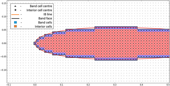
FIGURE 1. Cell classification.

The solution at the band faces is then reconstructed (solution forcing) to implicitly obey the desired boundary conditions at the immersed surface. Specifically, the boundary conditions considered for velocity forcing are no-slip and no-penetration conditions for viscous flows and only no-penetration conditions for inviscid flows. The variable reconstruction at the band face center is performed by first constructing an interpolation point normal to the immersed surface, as discussed as follows. This is different from the approach adopted in the work of Ramakrishnan et al. (2016), wherein only the solution at the nearest field cell to the band face was used for the solution reconstruction at the band face. The modification in the solution forcing approach was carried out to avoid the dependence of the forcing method on the relative location of the band face center with respect to the immersed surface, as required in the previous method. The velocity reconstruction strategy adopted in Ramakrishnan et al. (2016) is described as follows for the benefit of the reader.

3.2 Velocity reconstruction: Early effort

This section describes the velocity reconstruction methodology proposed by Ramakrishnan et al. (2016), which is henceforward referred to as IBM(A). This velocity forcing at the band face is loosely based on the boundary conditions applied at ghost cells adjacent to walls in finite volume solvers on body-fitted grids. The reconstruction for the slip- and no-slip wall is outlined as follows.

3.2.1 Slip wall

The velocity reconstruction for the slip-wall case is as follows:

${\vec{u}}_{\mathit{face}}={\vec{u}}_F-\left(\left(1-\frac{d_{\mathit{face}}}{d_F}\right){\vec{u}}_F.{\widehat{n}}_{IB}\right){\widehat{n}}_{IB},(6)$

$d_{\mathit{face}}=\mathit{min}\left(0,d_{\mathit{face}}\right).(7)$

Here, ${\vec{u}}_{\mathit{face}}$ refers to the velocity at a band-face center, ${\vec{u}}_F$ is the velocity at the field cell center adjacent to the band face, and ${\widehat{n}}_{IB}$ is the outward normal vector to the IB line segment closest to the band face. Also, d_face and d_F are the minimum distances from a band face center and its adjacent field cell center, respectively, to the IB line segment nearest to the band face, as shown in Figure 2. As mentioned in the work by Ramakrishnan et al. (2016), when the band face center lies within the immersed boundary as shown in (Figure 3), this formulation tends to become unstable, and hence, a limiter was used (Eq. 7). However, as shown subsequently in this work, the method with the limiter still shows grid sensitivity, which is undesirable.

FIGURE 2

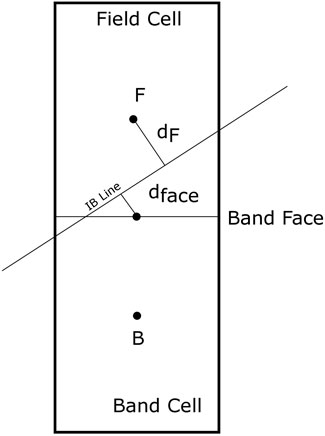
FIGURE 2. Distance nomenclature for the slip wall case.

FIGURE 3

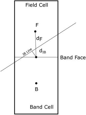
FIGURE 3. Distance nomenclature for the no-slip wall case.

3.2.2 No-slip wall

The velocity reconstruction for the no-slip wall case (Ramakrishnan et al., 2016) is as follows:

${\vec{u}}_{\mathit{face}}=\frac{\frac{{\vec{u}}_{\Vert F}}{d_F}+\frac{{\vec{u}}_{\Vert IB}}{d_{IB}}}{\frac{1}{d_F}+\frac{1}{d_{IB}}},(8)$

where

${\vec{u}}_{\Vert F}={\vec{u}}_F-\left({\vec{u}}_F.{\widehat{n}}_{IB}\right){\widehat{n}}_{IB}(9)$

and

${\vec{u}}_{\Vert IB}={\vec{u}}_{IB}-\left({\vec{u}}_{IB}.{\widehat{n}}_{IB}\right){\widehat{n}}_{IB}.(10)$

An inverse distance-based approach is used for the parallel component of velocity, whereas the perpendicular component of the velocity was considered zero (Ramakrishnan et al., 2016). The parallel and perpendicular directions considered are with respect to the nearest IB line to the band face. Here, ${\vec{u}}_{\mathit{face}}$ and ${\vec{u}}_F$ are as defined in the previous section, and ${\vec{u}}_{IB}$ refers to the velocity of the IB, which is zero for stationary boundaries.

The present work aims to avoid the use of any ad hoc limiting used in the aforementioned formulation (Eq. 7) for slip-wall cases and also presents a no-slip wall formulation that accounts for the perpendicular component of the velocity. A fix provided in the work by Rangan and Ghosh (2021) that avoids the use of the limiter led to the use of non-local forcing for some “band” faces and associated complexities with different treatments of band faces based on their relative location to the immersed boundary. In addition, the present formulation is devised such that the interpolation stencil used includes more number of cells than that used by Rangan and Ghosh (2021). The proposed formulation is explained in the following section(s).

3.3 Determination of the interpolation point

In this work, we construct an interpolation point on the line passing through the band-face center and normal to the nearest immersed surface (line segment). The distance of the interpolation point from the solution forcing point (which can be a face center or cell center) is often fixed for the entire domain as a function of local grid spacing(s) (Chi et al., 2017) or a fixed value as in the study by Capizzano (2011). In this work, however, to determine the position of the interpolation point, an interpolation stencil of nine cells is constructed, which consists of the field cell that has the band face and its eight neighbors. This ensures that more number of field cells are used in interpolating the primitive variables at the interpolation point. An inverse distance approach proposed by Ghosh et al. (2010) is then used to first determine the location of the interpolation point.

To do this, the perpendicular distances of the field cell centers from the line passing through the band face center and normal to the nearest IB line segment (for instance, $d_{p_i}$), as shown in Figure 4, are determined. Using the inverse of these distances as weights and the distance along the line (for instance, $d_{n_i}$) as the variable, the distance of the interpolation point from the band face center along the line is determined. Finally, the primitive variables are also interpolated at the interpolation point based on the same algorithm by using the nearby fluid cell data.

FIGURE 4

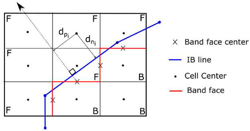
FIGURE 4. Stencil for the determination of the interpolation point.

The formulation is as shown as follows, wherein k is the total number of field cells in the 3 × 3 stencil considered. Here, d_n,IP is the distance of the interpolation point from the band face center along the normal line; ϕ_IP and ϕ_i are scalars (velocity components, pressure, and density) at the interpolation point and the field cell centers in the stencil, respectively.

$d_{n,IP}=\frac{{\sum }_{i=1}^k{w}_i{d}_{n_i}}{{\sum }_{i=1}^k{w}_i},(11)$

${\varphi }_{IP}=\frac{{\sum }_{i=1}^k{w}_i{\varphi }_i}{{\sum }_{i=1}^k{w}_i},(12)$

$w_i=\frac{1}{d_{p_i}},i=1:k.$

3.4 Solution reconstruction at the band face center

The basic idea here is to reconstruct the state at the band face such that the presence of the immersed boundary is “felt” by the rest of the flow. This is carried out by using the state (or some gradient information) of the flow variable at the immersed boundary and the data reconstructed at the interpolation point.

3.4.1 Velocity reconstruction–slip wall

For the reconstruction of the velocity at any band face, the velocity vector is split into components parallel and perpendicular to the nearest immersed surface. The velocity vector at some arbitrary point (ξ) in the neighborhood of the immersed surface is split into components shown as follows.

${\vec{u}}_{\xi }={\vec{u}}_{\Vert ,\xi }+{\vec{u}}_{\perp ,\xi },$

where

${\vec{u}}_{\perp ,\xi }=\left({\vec{u}}_{\xi }\cdot {\widehat{n}}_{IB}\right){\widehat{n}}_{IB}$

and

${\vec{u}}_{\Vert ,\xi }={\vec{u}}_{\xi }-{\vec{u}}_{\perp ,\xi }.$

Here, ${\widehat{n}}_{IB}$ is the unit vector drawn at a band face center along the line normal to the nearest immersed surface.

For the slip wall, the parallel component of the velocity at the band face is kept the same as the parallel component at the interpolation point, and the perpendicular component of the velocity is linearly interpolated to satisfy no penetration boundary condition on the IB surface. Thus,

${\vec{u}}_{\Vert face}={\vec{u}}_{\Vert IP},(13)$

${\vec{u}}_{\perp face}=\frac{d_{\mathit{face}}}{d_{IP}}{\vec{u}}_{\perp IP}.(14)$

This leads to the following equation for the velocity vector at the band face for the slip-wall case:

${\vec{u}}_{\mathit{face}}={\vec{u}}_{IP}-\left(\left(1-\frac{d_{\mathit{face}}}{d_{IP}}\right){\vec{u}}_{IP}\cdot {\widehat{n}}_{IB}\right){\widehat{n}}_{IB}.(15)$

3.4.2 Velocity reconstruction–no-slip wall

In the case of the no-slip wall, both the parallel and perpendicular components of the velocity on the IB surface should be zero. To achieve the same, a linear interpolation of the velocity components along the normal line is considered in this case to determine the solution forcing at the band face shown as follows.

${\vec{u}}_{\mathit{face}}=\frac{d_{\mathit{face}}}{d_{IP}}{\vec{u}}_{IP}.(16)$

A point to note is that the distances considered for the velocity reconstruction, in Eqs. 15, 16, are signed distances. The same is shown in Figure 5.

FIGURE 5

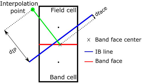
FIGURE 5. Schematic representation showing the distances used in face reconstruction.

3.4.3 Pressure and density reconstruction

Both the pressure and density at the face are set equal to the values at the fluid cell that shares the band face. This enforces the adiabatic wall boundary condition at the immersed surface.

$p_{\mathit{face}}=p_F,$

${\rho }_{\mathit{face}}={\rho }_F.$

3.4.4 Gradient at band faces

Since the primitive variables are reconstructed at the band face center, gradients are to be updated accordingly using the reconstructed band-face data. For viscous flows, the gradients at band faces are recomputed for the velocity components and temperature. The gradient is constructed as

$\vec{\nabla }\varphi =\frac{2\left({\varphi }_F-{\varphi }_{\mathit{face}}\right)}{0.5\left(V_F+V_B\right)}{A}_{\mathit{face}}{\widehat{n}}_{\mathit{face}},(17)$

$\varphi =u,v,T.$

V_F = Volume of the field cell

V_B = Volume of the band cell

Here, the direction of the normal vector ${\widehat{n}}_{\text{face}}$ is from the band-face center to the field cell center.

3.4.5 Higher-order spatial reconstruction

Implementation of higher-order data reconstruction at the cell faces near the immersed boundary needs some attention. This is so, as reconstruction at the faces using a second- or higher-order method uses at least the two adjacent cell data for any interface. This can pose a problem in IB methods since not all the cells contain physically correct data. In the present method, higher-order reconstruction at a cell face opposite to a band face requires the use of interior cell data, which needs to be addressed. In this work, we revert to first-order data reconstruction at such cell faces. To illustrate the same, the schematics shown in Figure 6 are considered. To reconstruct the data at face $(i+\frac{1}{2})$, the solution at the cells on either sides of the face is considered in general. However, for the present IB method, as shown in Figure 6, reconstructing the data at $(i+\frac{1}{2})$, L would require at least the adjacent band cell (i − 1) and possibly also the interior cell (i − 2) data, which is not appropriate. Hence, first-order reconstruction is adopted in this case.

FIGURE 6

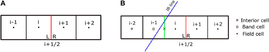
FIGURE 6. Standard stencil used for MUSCL (A) and MUSCL with the IBM (B).

Standard MUSCL reconstruction (Hirsch, 2007) is mentioned in Eqs 18 and 19, wherein the left and right states of a face are reconstructed using three adjacent cells. Here, ϕ is a higher-order switch, κ is a parameter that determines the order of the accuracy of the reconstruction, and ψ is the limiter function that limits the solution gradients to prevent oscillations in the solution. However, in the present IBM, the MUSCL algorithm is implemented as per Eqs 20 and 21 at the i + 1/2 interface (shown in Figure 6) to avoid using any interior cell data. This reduces the order of accuracy of reconstruction to first order at these faces.

$q_{i+\frac{1}{2}}^{\text{L}}=q_i+\frac{\varphi }{4}\left[\left(1-\kappa \right)\psi \left(\frac{{\mathrm{\Delta }}_{i}q}{{\nabla }_{i}q}\right){\nabla }_{j}q+\left(1+\kappa \right)\psi \left(\frac{{\nabla }_{i}q}{{\mathrm{\Delta }}_{i}q}\right){\mathrm{\Delta }}_{j}q\right],(18)$

$q_{i+\frac{1}{2}}^{\text{R}}=q_{i+1}+\frac{\varphi }{4}\left[\left(1+\kappa \right)\psi \left(\frac{{\mathrm{\Delta }}_{i}q}{{\nabla }_{i}q}\right){\nabla }_{j}q+\left(1-\kappa \right)\psi \left(\frac{{\nabla }_{i}q}{{\mathrm{\Delta }}_{i}q}\right){\mathrm{\Delta }}_{j}q\right],(19)$

$q_{i+\frac{1}{2}}^{\text{L}}=q_i,(20)$

$q_{i+\frac{1}{2}}^{\text{R}}=q_{i+1}+\frac{\varphi }{4}\left[\left(1+\kappa \right)\psi \left(\frac{{\mathrm{\Delta }}_{i}q}{{\nabla }_{i}q}\right){\nabla }_{j}q+\left(1-\kappa \right)\psi \left(\frac{{\nabla }_{i}q}{{\mathrm{\Delta }}_{i}q}\right){\mathrm{\Delta }}_{j}q\right],(21)$

where

${\mathrm{\Delta }}_{i}q=q_{i+1}-q_i,$

${\nabla }_{i}q=q_i-q_{i-1},$

$q=\left[\rho ,u,v,w,P\right].$

4 Results and discussion

The performance of the proposed IBM is assessed on the test cases listed in Table 1 by comparing it with the results from the existing literature. These include two transonic and two supersonic cases. For all the cases, Cartesian grids have been used. However, first, the performance comparison of the method in Ramakrishnan et al. (2016) and the present IBM is evaluated for flow past a bump in a channel. The computations are carried out on two grid sizes to investigate whether the grid size affects the stability of the algorithms.

TABLE 1

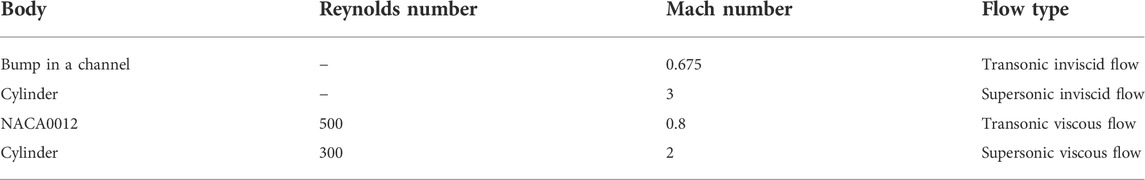
TABLE 1. Summary of test cases.

4.1 Bump in a channel

This test case simulates the inviscid transonic flow past a bump in a channel. The channel is 3.0 m long and 1.0 m in height. The bump is located halfway along the length of the lower wall. The thickness-to-chord ratio of the bump is 10%.

This internal flow test case was performed on a structured body-fitted grid by Favini et al. (1996), and the solution is compared with the same work. This simulation is carried out on grids with dimensions 130 × 42 and 180 × 64, for comparison of the present method with that presented in Ramakrishnan et al. (2016), and a sequence of successively refined grids 48 × 16, 96 × 32, 192 × 64, and 384 × 128 in the x and y directions, respectively, with clustering near the ends of the bump and minimum grid spacing—Δx_min = Δy_min = 0.005 m for the 192 × 64 grid—same as in Kumar et al. (2020). The inlet Mach number, pressure, and temperature are equal to 0.675, 1.0e5 Pa, and 300 K, respectively.

Boundary conditions applied are shown in Figure 7. The non-uniform mesh is shown in Figure 8 with the IB rendered as a yellow curve. The pressure contours obtained using the IBM from Ramakrishnan et al. (2016), referred to henceforward as IBM(A), and the present IBM are compared in Figure 9.

FIGURE 7

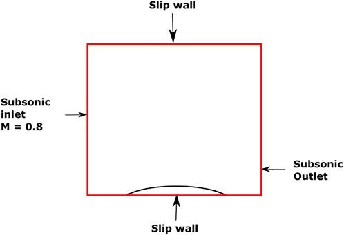
FIGURE 7. Schematic representation of the domain with boundary conditions indicated: transonic flow over bump in a channel.

FIGURE 8

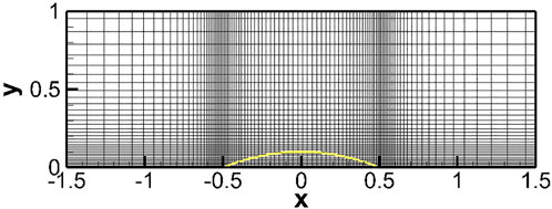
FIGURE 8. Non-uniform mesh used for transonic flow over a bump in a channel of size (192 × 64) in x and y directions, respectively (alternate grid lines are shown in both directions for clarity); IB shown by the yellow line.

FIGURE 9

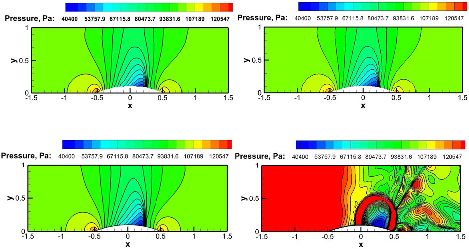
FIGURE 9. Pressure contour comparison for transonic flow over a bump using the present IBM and IBM(A). The present IBM (top) and IBM(A) (bottom); grid size: 130 × 42 (left) and 180 × 64 (right).

The contours indicate that both the IBM(A) and the proposed IBM produce similar results with the 130 × 42 grid. However, as the number of grid points is increased to 180 × 64, the solution using IBM(A) becomes non-physical whereas the present IBM generates physically correct results. It is to be noted that this incorrect behavior of the IBM(A) is present in spite of using the limiting function Eq. 7. Without the limiting function, the solution diverges.

The solution convergence with grid refinement can be observed from the surface plots of the Mach number in Figure 10A with the 192 × 64 grid and 384 × 128 grids having virtually identical surface Mach number distribution. Also, as shown in Figure 10B, the Mach number plots along the lower and upper surfaces of the domain (192 × 64) show overall excellent agreement with the results obtained by Favini et al. (1996).

FIGURE 10

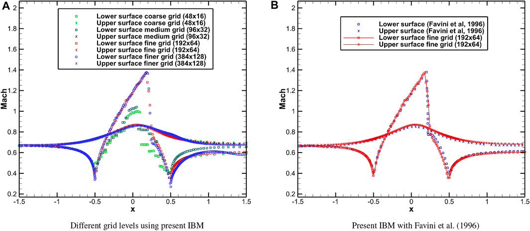
FIGURE 10. Mach number distribution on the upper and lower walls for transonic flow over a bump. (A) Different grid levels using present IBM. (B) Present IBM with Favini et al. (1996).

Figure 11 shows the pressure contour plots for the present computations and the CUS-IBM (Kumar et al., 2020) solution on the 192 × 64 grid. The shock structure and location show good agreement between the solvers, with the present solver producing a somewhat smeared shock foot.

FIGURE 11

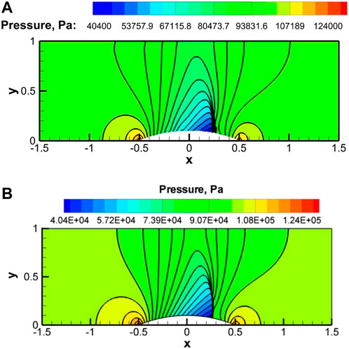
FIGURE 11. Pressure contours using the present IBM (A) and CUS-IBM (Kumar et al., 2020) (B) for the transonic flow over a bump.

The exit Mach number is probed at the lower and upper surfaces (listed in Table 2) and is compared against the body-fitted grid values obtained by Favini et al. (1996). The percentage errors for the lower and upper surfaces are 2.3 % and 2.54%, respectively.

TABLE 2

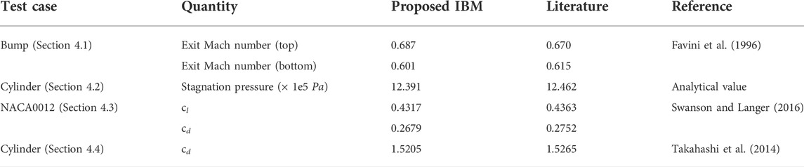
TABLE 2. Summary of the quantitative comparison of specific quantities obtained using the proposed IBM with the literature.

4.2 Inviscid supersonic flow past a circular cylinder

This is an external flow computation of flow over a cylinder. A supersonic flow of M_inlet = 3, P_inlet = 103320 Pa, and T = 300 K over a half-cylinder is simulated. The computational domain is [ −1 m, 0 m] × [ −2 m, 2 m]. The cylinder is centered at (0 m, 0 m) with a radius of 0.5 m.

Uniform Cartesian grids are chosen with grid sizes 50 × 200, 100 × 400, and 200 × 800 along the x and y directions, respectively, which are the same as reported in Kumar et al. (2020). A symmetry or slip-wall boundary condition is used for the top and bottom boundaries as the flow is expected to be parallel near these boundaries, with the bow shock exiting the right boundary. Boundary conditions used are as shown in Figure 12.

FIGURE 12

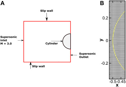
FIGURE 12. Schematic representation of the domain with boundary conditions indicated (A) and near-view of the grid showing every other pair of grid lines (B); IB shown by the yellow line.

Figure 13A plots the pressure coefficient along the surface of the upper-right quarter of the cylinder on different grids. It can be observed that the pressure distribution on the fine and medium grids is close to each other compared to that on the coarse grid, which suggests that the solution on the fine grid can be considered to be grid-converged. A comparison is also made between the grid-converged solution on the fine grid (200 × 800) using the present IBM and the results of the CUS-IBM (Kumar et al., 2020) on the same grid. Good agreement between the predictions can be seen, as shown in Figure 13B.

FIGURE 13

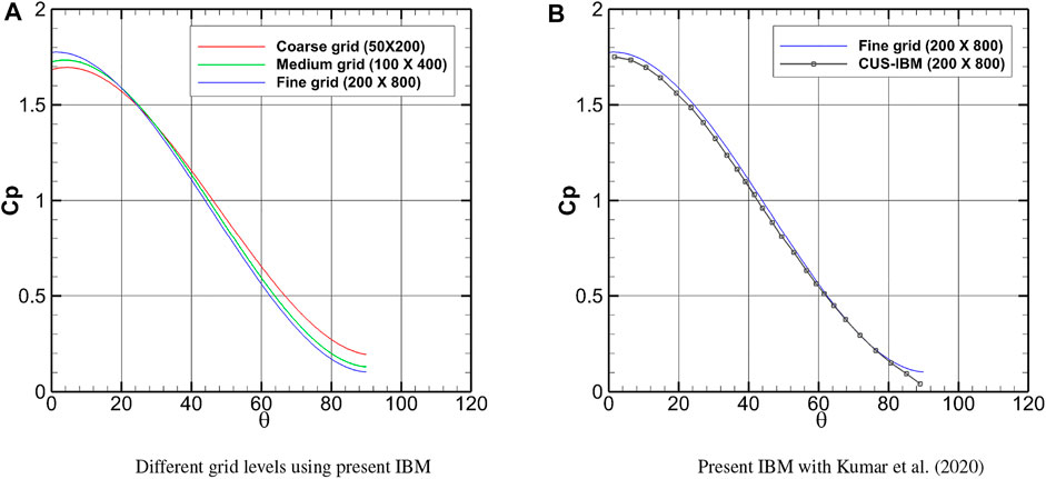
FIGURE 13. Comparison of the pressure coefficient; X-axis represents the azimuth angle measured clockwise from the leading edge. (A) Different grid levels using present IBM. (B) Present IBM with Kumar et al. (2020).

Furthermore, post-shock stagnation pressure in the computational domain is also probed at y = 0 and compared to the calculated analytical value (listed in Table 2). The percentage error of the computed value is determined to be about 0.57%. The contour plot of the Mach number is shown in Figure 14, and a comparison is also made with the CUS-IBM (Kumar et al., 2020). The contour plots are in good agreement. It can be seen from the contours that there is a detached bow shock formed in front of the cylinder, and the solutions on the two different IBM solvers compare well.

FIGURE 14

FIGURE 14. Mach number contour comparison–present IBM (A) and CUS-IBM (Kumar et al., 2020) (B).

4.3 Transonic viscous flow past the NACA0012 airfoil

This is a laminar flow simulation with a large separation vortex near the trailing edge of the airfoil. Free stream flow parameters are M_∞ = 0.8, p_∞ = 103320 Pa, T_∞ = 300 K, and Re_∞ = 500, and the angle of attack is 10°.

This test case is chosen as the flow is transonic and involves flow separation with a recirculation bubble forming on the suction side of the airfoil. This tests whether the IBM can accurately predict flow separation, which is very important for the reliable prediction of viscous flows.

The computations for this case are carried out on the non-uniform grids of sizes 162 × 256, 324 × 512, and 648 × 1,024 along x and y directions, respectively. The size of the grid 648 × 1,024 is based on the grid used in Kumar et al. (2020), with a minimum grid spacing of Δx_min = Δy_min = 0.005 m at the leading edge. Boundary conditions considered and the zoomed-in view of the grid used are shown in Figure 15. The solution of the present IB method is compared with the body-fitted grid simulation by Swanson and Langer (2016).

FIGURE 15

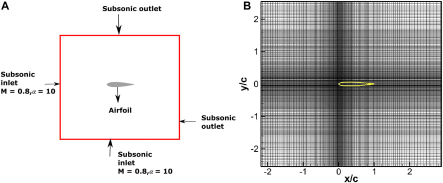
FIGURE 15. Schematic representation of the domain with boundary conditions indicated: flow past airfoil NACA0012 (A) and close-up view of the 648 × 1,024 non-uniform mesh (B) (showing alternate grid lines in both directions); IB shown by the yellow line.

Figure 16A shows the grid convergence results obtained using the presented IB method. It can be observed that the surface pressure coefficient predictions on both the medium and fine grids overlap, and the solution on the 648 × 1,024 grid can be considered as grid-converged. In Figure 16B, pressure coefficient distribution on the airfoil with the present IBM (648 × 1,024) is further compared with the 1,280 × 512 C grid computations by Swanson and Langer (2016). The C_p distributions for the two methods match closely, indicating that the computations with the present IBM produce accurate surface pressure with a grid having a similar size as used for a body-fitted simulation.

FIGURE 16

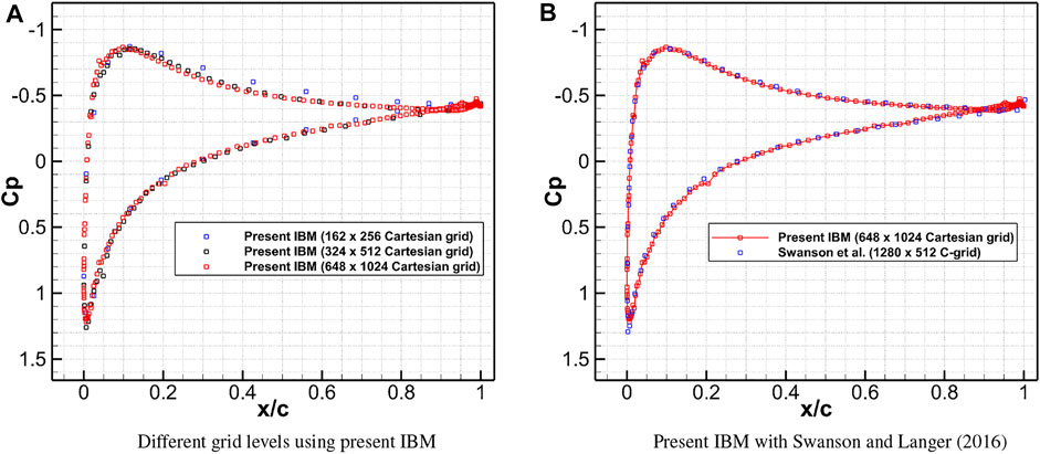
FIGURE 16. Comparison of surface pressure distribution for transonic flow over the airfoil. (A) Different grid levels using present IBM. (B) Present IBM with Swanson and Langer (2016).

As can be seen from Figure 17, which presents the Mach number contour plots using the present IBM and body-fitted grid simulations (Swanson and Langer, 2016), there is good agreement between the predicted solutions. In Figure 18, streamlines are shown in a zoomed-in view of the region near the trailing edge to compare the predictions of the recirculation zone between the present IBM and body-fitted simulation by Swanson and Langer (2016). It can be observed that the location and size of the recirculation regions look very similar. Furthermore, the errors in the lift coefficient c_l and the drag coefficient c_d, between the present computation and value reported by Swanson and Langer (2016) using body-fitted grid simulations, are determined to be about 1.07% and 2.6%, respectively. The exact values of the lift and drag coefficients are listed in Table 2.

FIGURE 17

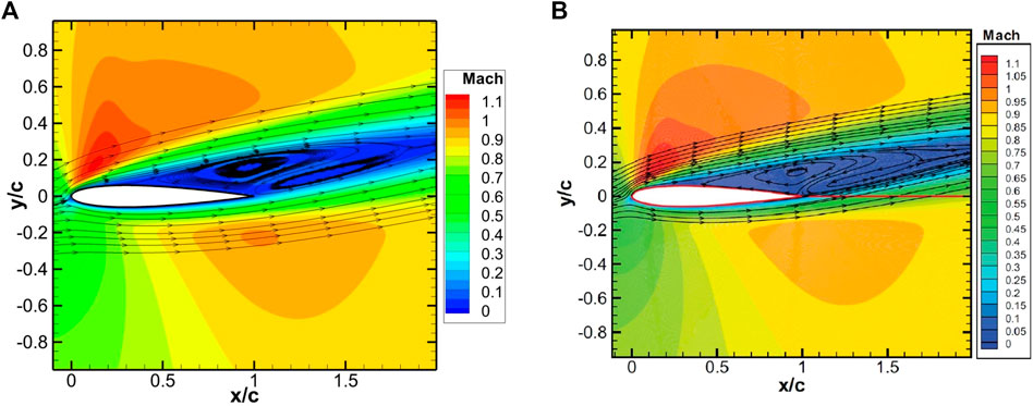
FIGURE 17. Comparison of Mach number contours for the transonic flow past the NACA0012 airfoil. Present IBM (A) and the IBM of Swanson and Langer (2016) (B).

FIGURE 18

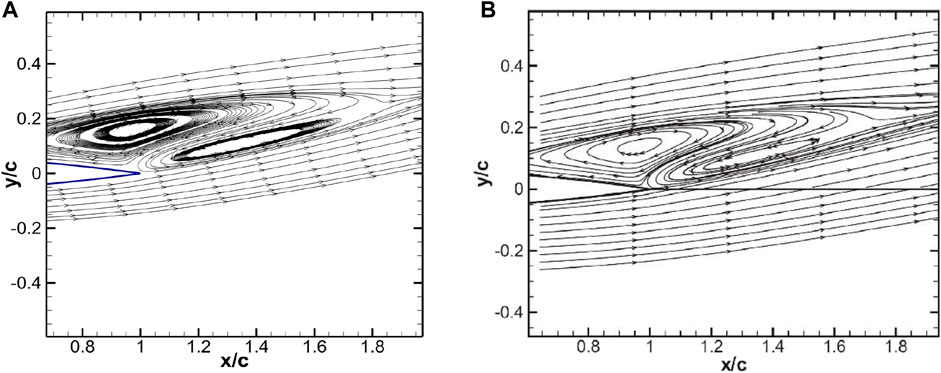
FIGURE 18. Streamlines showing separation bubbles for the transonic viscous flow past the NACA0012 airfoil: present IBM (A) and the IBM of Swanson and Langer (2016) (B).

4.4 Supersonic viscous flow past the cylinder

Flow conditions for this external flow simulation are M_∞ = 2.0, p_∞ = 103320 Pa, T_∞ = 300 K, and Re = 300. The domain extent is 60 D × 40 D (D = 1 m), the same as in Kumar et al. (2020) and Qiu et al. (2016), and the cylinder is centered at (24,20).

Non-uniform meshes with grid sizes 158 × 108, 316 × 216, and 632 × 432 along x and y directions, respectively, were used for the grid convergence study. There is a uniform mesh region around the cylinder of size 1.7 D × 1.7 D with a grid spacing of 0.1 D, 0.05 D, and 0.025 D for three levels of grids as in Takahashi et al. (2014). This grid spacing of the finest grid used is considered sufficient to capture the boundary layer effects for the specific Reynolds number. The domain with the boundary conditions employed and the grid are shown in Figure 19.

FIGURE 19

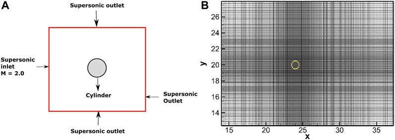
FIGURE 19. Schematic representation of the domain with boundary conditions indicated (A) and close-up view of the non-uniform grid (B) (showing alternate grid line in both directions); IB shown by the yellow line.

As shown in Figure 20A, it can be observed that the predicted pressures on the medium and fine grids are virtually overlapping, and thus, the solution on the 632 × 432 grid can be considered as grid-converged.

FIGURE 20

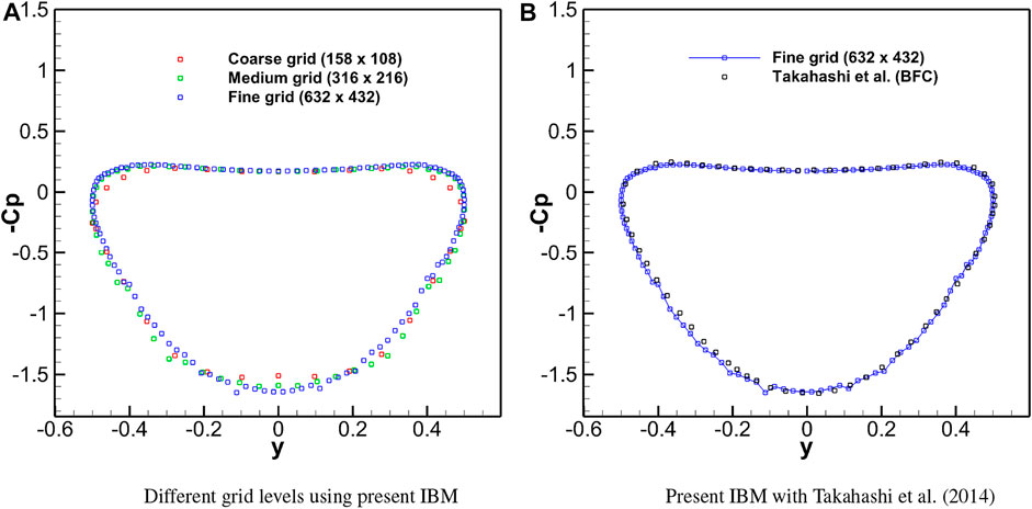
FIGURE 20. Comparison of surface pressure distribution for the supersonic flow over a cylinder. (A) Different grid levels using present IBM. (B) Present IBM with Takahashi et al. (2014).

The pressure coefficient on the cylinder surface plotted in Figure 20B compares the converged solution on the finer grid with the published results by Takahashi et al. (2014) and shows excellent agreement.

Furthermore, the error in the drag coefficient, c_d, between the present computation and the value reported by Takahashi et al. (2014) for Cartesian grid simulations is determined to be about 0.4%. The exact values of the lift and drag coefficients are listed in Table 2. Contour plots of the density ratio in Figure 21 show that the bow shock is captured well with the present IBM and the flow field is qualitatively similar to that predicted by Takahashi et al. (2014).

FIGURE 21

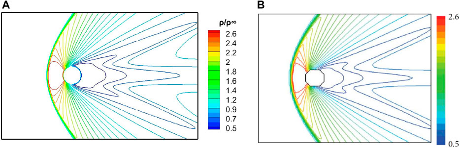
FIGURE 21. Density contour plot using the present IBM (A) and the IBM of Takahashi et al. (2014) (B).

4.5 Performance study

This section discusses the performance of the proposed IB solver by performing grid convergence tests on three grids of different sizes for two of the test cases presented earlier in this work: inviscid Mach 3 flow past a circular cylinder and viscous Mach 2.0 flow past a circular cylinder at Re of 300. For the inviscid flow test case, the three grids considered are 50 × 200, 100 × 400, and 200 × 800 on the computational domain of [−1,0]×[−2,2] with uniform grid spacing. For the viscous flow simulations, the three grid sizes chosen are 158 × 108, 316 × 216, and 632 × 432 with a uniform grid spacing of 0.1 D, 0.05 D, and 0.025 D, respectively, in the rectangular region 1.7 × 1.7 around the cylinder.

For the inviscid test case, post-shock stagnation pressure along the line y = 0 is considered to determine the error in the computation. The reference value in this case is the theoretical post normal-shock value at Mach 3.0 for air. For the viscous test case, the error in the solution is calculated by computing the drag coefficient C_d. An error function is computed as ${ϵ}_h=\frac{|\varphi -{\varphi }_{\mathit{ref}}|}{\varphi ref}$, where ϕ = [P₀, C_D] and ϕ_ref is the zero-grid-spacing reference value, obtained using Richardson’s extrapolation (Slater, 2022, Roache, 1994). The plot shown in Figure 22 shows the variation of the error function (ϵ_h) epsilon versus the grid spacing parameter (r). The grid spacing parameter r is defined as the ratio of the average grid spacing of a grid with respect to the average grid spacing for the finest grid. The observed order of convergence obtained is in the range of 1.4–1.6, which is determined using that of Slater (2022). This suggests that the solution obtained from the proposed IBM is less than second-order accurate, although the finite volume method used here is second-order accurate. This can be attributed to the reduced order of solution reconstruction at cell faces in the neighborhood of the immersed surface, as discussed in Section 3.4.5. Furthermore, although linear interpolation is used for forcing the velocity at the band face, density and pressure are extrapolated, which can also contribute to the overall reduction in the accuracy of the solver.

FIGURE 22

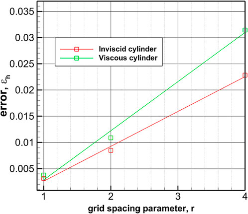
FIGURE 22. Variation of ϵ with an average grid spacing parameter (r) for the supersonic inviscid flow past the cylinder (red) and the viscous flow past the cylinder (green).

5 Conclusion

An immersed boundary method designed for the finite volume solver of the equations of the fluid flow is presented in this work. Specifically, this work presents a robust face-based solution forcing methodology in the immediate vicinity of the immersed surface, which enables the integration of the discretized equations in all the fluid cells, thus allowing better adherence to the conservation of mass, momentum, and energy. An interpolation point is constructed along the normal to the immersed surface, and data are interpolated from the surrounding fluid cells onto the interpolation point using inverse distances as weights. The proposed methodology has been validated with simulations of the flow past a bump, cylinder, and airfoil with speeds ranging from transonic to supersonic regime, both laminar and inviscid. The results presented indicate that the flow predictions away from the immersed surface and surface pressure compare well with results reported in the literature. Quantitative comparison with results from the literature/theoretical values shows that the errors in the present method are less than 3%. Subsequent development will be aimed at moving boundary modifications, extending to three dimensions, and improving geometric conservation.

Data availability statement

The raw data supporting the conclusion of this article will be made available by the authors, without undue reservation.

Author contributions

MK: implementation of the algorithm, computation of numerical simulations, generation and presentation of results, and writing the manuscript. SG: proposed the overall formulation of the method and contributed to the writing and editing of the manuscript.

Conflict of interest

The authors declare that the research was conducted in the absence of any commercial or financial relationships that could be construed as a potential conflict of interest.

Publisher’s note

All claims expressed in this article are solely those of the authors and do not necessarily represent those of their affiliated organizations, or those of the publisher, the editors, and the reviewers. Any product that may be evaluated in this article, or claim that may be made by its manufacturer, is not guaranteed or endorsed by the publisher.

References

Anand Bharadwaj, S., and Ghosh, S. (2020). Data reconstruction at surface in immersed-boundary methods. Comput. Fluids 196, 104236. doi:10.1016/j.compfluid.2019.104236

CrossRef Full Text | Google Scholar

Berthelsen, P. A., and Faltinsen, O. M. (2008). A local directional ghost cell approach for incompressible viscous flow problems with irregular boundaries. J. Comput. Phys. 227, 4354–4397. doi:10.1016/j.jcp.2007.12.022

CrossRef Full Text | Google Scholar

Brehm, C., Hader, C., and Fasel, H. (2015). A locally stabilized immersed boundary method for the compressible Navier–Stokes equations. J. Comput. Phys. 295, 475–504. doi:10.1016/j.jcp.2015.04.023

CrossRef Full Text | Google Scholar

Capizzano, F. (2007). “A compressible flow simulation system based on cartesian grids with anisotropic refinements,” in Collection of technical papers - 45th AIAA aerospace sciences meeting, 17036–17057. doi:10.2514/6.2007-1450

CrossRef Full Text | Google Scholar

Capizzano, F. (2011). Turbulent wall model for immersed boundary methods. AIAA J. 49, 2367–2381. doi:10.2514/1.J050466

CrossRef Full Text | Google Scholar

Chi, C., Lee, B. J., and Im, H. G. (2017). An improved ghost-cell immersed boundary method for compressible flow simulations. Int. J. Numer. Methods Fluids 83, 132–148. doi:10.1002/fld.4262

CrossRef Full Text | Google Scholar

Choi, J. I., Oberoi, R. C., Edwards, J. R., and Rosati, J. A. (2007). An immersed boundary method for complex incompressible flows. J. Comput. Phys. 224, 757–784. doi:10.1016/j.jcp.2006.10.032

CrossRef Full Text | Google Scholar

De Palma, P., de Tullio, M., Pascazio, G., and Napolitano, M. (2006). An immersed-boundary method for compressible viscous flows. Comput. Fluids 35, 693–702. doi:10.1016/j.compfluid.2006.01.004

CrossRef Full Text | Google Scholar

de Tullio, M., De Palma, P., Iaccarino, G., Pascazio, G., and Napolitano, M. (2007). An immersed boundary method for compressible flows using local grid refinement. J. Comput. Phys. 225, 2098–2117. doi:10.1016/j.jcp.2007.03.008

CrossRef Full Text | Google Scholar

Edwards, J. R., Choi, J., Ghosh, S., Gieseking, D. A., and Eischen, J. D. (2010). “An immersed boundary method for general flow applications,” in ASME 2010 3rd joint US-European fluids engineering summer meeting: Volume 1, symposia – Parts A, B, and C of fluids engineering division summer meeting, 2461–2469. doi:10.1115/FEDSM-ICNMM2010-31097

CrossRef Full Text | Google Scholar

Ehsan Khalili, M., Larsson, M., and Müller, B. (2018). Immersed boundary method for viscous compressible flows around moving bodies. Comput. Fluids 170, 77–92. doi:10.1016/j.compfluid.2018.04.033

CrossRef Full Text | Google Scholar

Fadlun, E. A., Verzicco, R., Orlandi, P., and Mohd-Yusof, J. (2000). Combined immersed-boundary finite-difference methods for three-dimensional complex flow simulations. J. Comput. Phys. 161, 35–60. doi:10.1006/jcph.2000.6484

CrossRef Full Text | Google Scholar

Favini, B., Broglia, R., and Di Mascio, A. (1996). Multigrid acceleration of second-order eno schemes from low subsonic to high supersonic flows. Int. J. Numer. Methods Fluids 23, 589–606. doi:10.1002/(sici)1097-0363(19960930)23:6<589:aid-fld444>3.0.co;2-#

CrossRef Full Text | Google Scholar

Gao, T., Tseng, Y.-H., and Lu, X.-Y. (2007). An improved hybrid cartesian/immersed boundary method for fluid-solid flows. Int. J. Numer. Methods Fluids 55, 1189–1211. doi:10.1002/fld.1522

CrossRef Full Text | Google Scholar

Ghias, R., Mittal, R., and Dong, H. (2007). A sharp interface immersed boundary method for compressible viscous flows. J. Comput. Phys. 225, 528–553. doi:10.1016/j.jcp.2006.12.007

CrossRef Full Text | Google Scholar

Ghosh, S., and Anand Bharadwaj, S. (2020). Development and application of immersed boundary methods for compressible flows. Singapore: Springer Singapore, 227–249. doi:10.1007/978-981-15-3940-4_8

CrossRef Full Text | Google Scholar

Ghosh, S., Choi, J. I., and Edwards, J. R. (2010). Numerical simulations of effects of micro vortex generators using immersed-boundary methods. AIAA J. 48, 92–103. doi:10.2514/1.40049

CrossRef Full Text | Google Scholar

Goldstein, D., Handler, R., and Sirovich, L. (1993). Modeling a No-slip flow boundary with an external force field. J. Comput. Phys. 105, 354–366. doi:10.1006/jcph.1993.1081

CrossRef Full Text | Google Scholar

Hartmann, D., Meinke, M., and Schröder, W. (2009). “A general formulation of boundary conditions on Cartesian cut-cells for compressible viscous flow,” in 19th AIAA Computational Fluid Dynamics Conference. doi:10.2514/6.2009-3878

CrossRef Full Text | Google Scholar

Hirsch, C. (2007). Numerical computation of internal and external flows: The fundamentals of computational fluid dynamics. 2 edn. Butterworth-Heinemann.

Google Scholar

Kim, J., Kim, D., and Choi, H. (2001). An immersed-boundary finite-volume method for simulations of flow in complex geometries. J. Comput. Phys. 171, 132–150. doi:10.1006/jcph.2001.6778

CrossRef Full Text | Google Scholar

Kitamura, K., Shima, E., Fujimoto, K., and Wang, Z. J. (2011). Performance of low-dissipation euler fluxes and preconditioned lu-sgs at low speeds. Commun. Comput. Phys. 10, 90–119. doi:10.4208/cicp.041109.160910a

CrossRef Full Text | Google Scholar

Kumar, V., Sharma, A., and Singh, R. K. (2020). Central upwind scheme based immersed boundary method for compressible flows around complex geometries. Comput. Fluids 196, 104349. doi:10.1016/j.compfluid.2019.104349

CrossRef Full Text | Google Scholar

Liou, M.-S., and Steffen, C. J. (1993). A new flux splitting scheme. J. Comput. Phys. 107, 23–39. doi:10.1006/jcph.1993.1122

CrossRef Full Text | Google Scholar

Luo, H., Baum, J. D., and Löhner, R. (2006). A hybrid cartesian grid and gridless method for compressible flows. J. Comput. Phys. 214, 618–632. doi:10.1016/j.jcp.2005.10.002

CrossRef Full Text | Google Scholar

Mittal, R., Dong, H., Bozkurttas, M., Najjar, F., Vargas, A., and von Loebbecke, A. (2008). A versatile sharp interface immersed boundary method for incompressible flows with complex boundaries. J. Comput. Phys., 227, 4825–4852. Cited by: 799; All Open Access, Green Open Access. doi:10.1016/j.jcp.2008.01.028

PubMed Abstract | CrossRef Full Text | Google Scholar

Mohd-Yusof, J. (1997). Combined immersed-boundary/b-spline methods for simulations of flow in complex geometries. Cent. Turbul. Res. Annu. Res. briefs 161, 317–327.

Google Scholar

Peskin, C. S., and McQueen, D. M. (1989). A three-dimensional computational method for blood flow in the heart I. Immersed elastic fibers in a viscous incompressible fluid. J. Comput. Phys. 81, 372–405. doi:10.1016/0021-9991(89)90213-1

CrossRef Full Text | Google Scholar

Peskin, C. S. (1972). Flow patterns around heart valves: A numerical method. J. Comput. Phys. 10, 252–271. doi:10.1016/0021-9991(72)90065-4

CrossRef Full Text | Google Scholar

Peskin, C. S. (1977). Numerical analysis of blood flow in the heart. J. Comput. Phys. 25, 220–252. doi:10.1016/0021-9991(77)90100-0

CrossRef Full Text | Google Scholar

Qiu, Y., Shu, C., Wu, J., Sun, Y., Yang, L., and Guo, T. (2016). A boundary condition-enforced immersed boundary method for compressible viscous flows. Comput. Fluids 136, 104–113. doi:10.1016/j.compfluid.2016.06.004

CrossRef Full Text | Google Scholar

Qu, Y., Shi, R., and Batra, R. C. (2018). An immersed boundary formulation for simulating high-speed compressible viscous flows with moving solids. J. Comput. Phys. 354, 672–691. doi:10.1016/j.jcp.2017.10.045

CrossRef Full Text | Google Scholar

Ramakrishnan, R., Girdhar, A., and Ghosh, S. (2016). “Immersed boundary methods for compressible laminar flows,” in VII European Congress on Computational Methods in Applied Sciences and Engineering, 7029–7044. doi:10.7712/100016.2315.8780

CrossRef Full Text | Google Scholar

Rangan, M. K., and Ghosh, S. (2021). “2D immersed boundary solver for compressible laminar flows,” in AIAA 2021-2729. AIAA AVIATION 2021 FORUM. doi:10.2514/6.2021-2729

CrossRef Full Text | Google Scholar

Roache, P. J. (1994). Perspective: A method for uniform reporting of grid refinement studies. J. Fluids Eng. 116, 405–413. doi:10.1115/1.2910291

CrossRef Full Text | Google Scholar

Sandhu, J. P. S., Girdhar, A., Ramakrishnan, R., Teja, R. D., and Ghosh, S. (2020). Fest-3d: Finite-volume explicit structured 3-dimensional solver. J. Open Source Softw. 5, 1555. doi:10.21105/joss.01555

CrossRef Full Text | Google Scholar

Seo, J. H., and Mittal, R. (2011). A sharp-interface immersed boundary method with improved mass conservation and reduced spurious pressure oscillations. J. Comput. Phys. 230, 7347–7363. doi:10.1016/j.jcp.2011.06.003

PubMed Abstract | CrossRef Full Text | Google Scholar

Slater, J. (2022). Examining spatial (grid) convergence. [Dataset]. Available at: https://www.grc.nasa.gov/www/wind/valid/tutorial/spatconv.html. (Accessed September 26, 2022).

Google Scholar

Swanson, R., and Langer, S. (2016). Steady-state laminar flow solutions for naca 0012 airfoil. Comput. Fluids 126, 102–128. doi:10.1016/j.compfluid.2015.11.009

CrossRef Full Text | Google Scholar

Takahashi, S., Nonomura, T., and Fukuda, K. (2014). A numerical scheme based on an immersed boundary method for compressible turbulent flows with shocks : Application to two-dimensional flows around cylinders. J. Comput. Appl. Math. 2014, 21. doi:10.1155/2014/252478

CrossRef Full Text | Google Scholar

Tamaki, Y., and Imamura, T. (2018). Turbulent flow simulations of the common research model using immersed boundary method. AIAA J. 56, 2271–2282. doi:10.2514/1.j056654

CrossRef Full Text | Google Scholar

Tseng, Y. H., and Ferziger, J. H. (2003). A ghost-cell immersed boundary method for flow in complex geometry. J. Comput. Phys. 192, 593–623. doi:10.1016/j.jcp.2003.07.024

CrossRef Full Text | Google Scholar

Uhlmann, M. (2005). An immersed boundary method with direct forcing for the simulation of particulate flows. J. Comput. Phys. 209, 448–476. doi:10.1016/j.jcp.2005.03.017

CrossRef Full Text | Google Scholar