Validation of DSMC mass flow modeling for transsonic gas flows in micro-propulsion systems

1 Introduction

Modeling nozzle flows is a common problem in the development of new propulsion systems for space applications. Due to the vacuum conditions of a space environment, the flow cases of interest are often in a rarefied flow regime. Flow conditions from slip flow (0.001 < Kn < 0.1) to transition flow (0.1 < Kn < 10) to free flow (Kn > 10) are generated. The Direct Simulation Monte Carlo (DSMC) method, described by G.A. Bird in this 1994 monograph (Bird, 1994), is a widely used tool for simulating diluted flow fields in all types of geometries. The method has been used to simulate re-entering space capsules (Shang and Chen, 2013), micro-electromechanical systems (MEMS) (Alexeenko et al., 2002; Wang and Li, 2004), or nozzle geometries, and plume effects (Ivanov et al., 1997; Arlemark et al., 2012), and has been shown to correctly solve flow problems where continuum approaches fail due to the strong effects of flow rarefaction.

In more traditional DSMC benchmarks (Bird, 2007) and simulations, velocity driven boundary conditions are often used to model the inflow and outflow of the numerical domain. For example, to model supersonic free flow environments enclosing the geometry of interest. However, this boundary condition treatment requires a large flow field to be modeled, with boundaries far from the geometry (Nance et al., 1997; Liou and Fang, 2000). Later, the first investigations of heat transfer descriptions with implicit boundary condition were carried out using DSMC methods (Fang and Liou, 2002).

The flow temperature, density, and velocity at the boundaries must be known. In contrast, the simulation of micronozzle, nozzle (Ivanov et al., 1999; Liu et al., 2006) and channel flow cases (Wang and Li, 2004; Roohi et al., 2009; Akhlaghi and Roohi, 2014) often exhibit subsonic inflow boundary conditions with inlet and in some cases outlet boundaries close to the studied geometry. In addition, the inlet and background pressure, inlet temperature, or mass flow rate are known from experimental nozzle flow setups rather than the inflow velocity or density.

A variety of approaches have been documented in the literature applying velocity driven inflow models to subsonic micro-geometry flows. For example, Wang and Li (Wang and Li, 2004) used what they called “1D characteristic theory” to extrapolate the inflow velocity, density, and temperature from the internal flow field. Their results for micro-Poisouille, orifice, and microchannel flows were in good agreement with experimental and theoretical values. The approach was also used to simulate subsonic gas flows through micro- and nanoscale channels (Roohi et al., 2009; Akhlaghi and Roohi, 2014) and nozzle (Darbandi and Roohi, 2011) flows. Another approach was taken by Ivanov et al. (Ivanov et al., 1997, 1999) who calculated the inflow velocity from isentropic relations for nozzle flows.

More advanced methods have been used to control flows using pressure and velocity boundary conditions (Farbar and Boyd, 2014; Lei et al., 2017). For large density gradients, collision selection methods allow a reduction in computational cost without loss of necessary precision (Frieler and Groll, 2023). Modern methods allow DSMC methods to model chemical reactions (Plotnikov and Shkarupa, 2021) and ionization processes (Kühn and Groll, 2021). In the present work, a new inflow model based on mass flow rate, temperature, and inflow area is presented. The approach is particularly suitable for arbitrary nozzle flow cases with higher density subsonic inflow conditions. Assuming a subsonic, slow inflow, the flow velocity is determined based on the pressure drop between the geometry and the Maxwellian velocity distribution of the molecules. The approach takes advantage of the precise knowledge of the inflow mass flow rate and temperature as a boundary condition, e.g., from experimental nozzle flow setups.

2 Materials and methods

2.1 Numerical method

DSMC (Direct Simulation Monte Carlo) is a statistical simulation method based on kinetic gas theory. The method, introduced by Bird (Bird, 1970; Bird, 1994), models gas flows by collision and statistical evaluation of test particles to solve the Boltzmann equation. In a simulation, each test particle carries the physical properties of a large number of real molecules advancing through the flow. A key element of the method is the consideration of only binary collisions and the decoupling of collision and motion of the test particles. This can be assumed in the case of a rarefied gas and when the simulation time step Δ t is smaller than the physical collision time t_c. Conservation of momentum and energy is achieved by additional interactions with the boundaries of the numerical domain.

After initialization at the beginning of a simulation, the test particles are moved according to their individual Maxwellian velocities and collisions are performed based on binary and wall collision models. When a cell boundary or open domain boundary is reached, the test particles are transferred or deleted. Sampling of macroscopic flow properties is then performed on the statistical basis of the test particles present in a cell over a number of time steps. These steps are repeated until a steady state is reached.

The mass flow driven inflow model presented and validated in this work was developed within the free software package OpenFOAM (OpenFOAM Ltd, 2016) using the DSMC solver dsmcfoam implemented by Scanlon et al. (Scanlon et al., 2010). The NTC (No Time Counter) scheme (Bird, 2007) is used to evaluate the number of collision pairs in a time step, as well as subcell generation to achieve nearest neighbor collisions within a cell (Bird, 2007). To model binary collisions, the variable hard sphere collision model (Bird, 1994) is used with the addition of Larsen-Borgnakke energy.

2.2 Mass flow driven inflow model

Following Bird’s original formulation, the inflow and outflow of the computational domain is modeled based on an equilibrium state formulation (Bird, 1994). In a simulation, the approach describes molecular flux quantities of an equilibrium gas across a surface between the computational domain and an associated virtual volume (Bird, 1994). The approach can be considered velocity driven, since a flow velocity must be set to produce a mass flow normal to the surface in a given direction. It is well suited for geometries in free flow environments, such as a re-entering space capsule (Shang and Chen, 2013).

However, in nozzle flow simulations, this treatment of mass flow at the entry and exit boundaries poses some challenges, since the exact flow velocity must be known in addition to temperature and number density. In contrast, the mass flow entering the engine is often a specified and controlled quantity in experimental setups. Thus, an inflow model based on this quantity would take advantage of the precise knowledge of the inflow mass flow rate as a boundary condition. In Figure 1 the physical inflow and outflow characteristics required by the present mass flow driven inflow model are shown as a flow chart. At the inlet, the mass flow rate must be known from the experiment, as well as the surface area of the inflow and the stagnation temperature of the case. The outflow is modeled by absolute pressure, temperature and velocity at some distance from the nozzle exit.In the model, the inflow particle flux ${\dot{N}}_{\text{in}}$ into the numerical domain is modeled as

${\dot{N}}_{\text{in}}=A_{\text{in}}{n}_{\text{in}},(1)$

in which A_in is the nozzle’s inlet cross section. The quantity n_in is directly derived from the mass flow rate ${\dot{m}}_{\text{in}}$ known from the experiment, the molar mass M of the used gas and the Avogadro constant N_A with

$n_{\text{in}}=\frac{{\dot{m}}_{\text{in}}}{A_{\text{in}}M{N}_A}.(2)$

to create a steady inflow of molecules across the inlet boundary, all molecules hitting an open domain boundary are additionally reflected. The molecular velocity of the test particles generated at the inlet is based on the Maxwellian velocity distribution for the given temperature T_in. Assuming a subsonic, slow inflow condition at the inflow boundary, the flow velocity is based on the pressure drop across the nozzle and the Maxwellian velocity distribution of the test particles after a certain distance in the downstream direction.

FIGURE 1

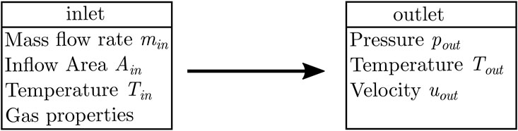
FIGURE 1. Physical in- and outflow properties of the present mass flow driven inflow model.

The outflow of the numerical domain is modeled on the basis of Bird’s equilibrium formulation (Bird, 1994) with

${\dot{N}}_{\text{out}}=\frac{A_{\text{out}}{n}_{\text{out}}{c}_{mp}\left[\exp \left(-q^2\right)+\sqrt{\pi }\left(1+\text{erf}\{q\}\right)\right]}{2\sqrt{\pi }}.(3)$

Here, c_mp is the most probable thermal velocity of a particle and n_out is the number density at the boundary. The most probable thermal velocity is given by the Boltzmann constant k_B, the macroscopic temperature T (= T_out) and the molecular mass m with

$c_{mp}=\sqrt{\frac{2k_{B}T}{m}}.(4)$

the term q in Eq. 3 is given by

$q=\frac{u_{\text{out}}}{c_{mp}}\cos \left(\theta \right),(5)$

with the local stream velocity u_out and the angle θ to the surface normal of the outflow boundary.

2.3 Rothe’s nozzle test case and mesh

Experimental data on flow properties in de Laval nozzles for low Reynolds numbers and high Knudsen numbers are hard to find. A well-known case is Rothe’s nozzle experiments (Rothe, 1971), where density and temperature data were measured inside a de Laval nozzle by an electron beam technique, analyzing the emission of the excited nitrogen molecules of the gas flow (Rothe, 1971; Rothe, 1965). The data have been used in a variety of numerical studies (Kim, 1994; Zelesnik et al., 1994; Chung et al., 1995; Ivanov et al., 1997; Arlemark et al., 2012), ranging from the 1970s to the present day, and are chosen as a test case to benchmark and validate the present inflow model.

Further comparison of numerical results of Rothe’s nozzle geometry, obtained by Ivanov et al. (Ivanov et al., 1999), are also considered, since their study includes results for both a Navier-Stokes solver GASP and a DSMC solver SMILE.

Rothe’s study covers several cases of nitrogen de Laval nozzle flows for two throat diameters, different mass flow rates, and varying nozzle pressure ratios between the stagnation chamber inside the nozzle and the background pressure of the vacuum chamber. Each case is specified by a so-called throat Reynold number notation

$B=\sqrt{2h_{\text{in}}}\frac{{\rho }_{\text{in}}}{{\mu }_{\text{in}}}{r}_{*},(6)$

where the stagnation chamber gas density and viscosity are ρ_in and μ_in, while the throat radius is represented by r*. The specific enthalpy given by h_in forms the adiabatic escape speed of the case with $\widehat{u}=\sqrt{2h_{\text{in}}}$.

The investigated nozzle geometry, shown in the lower part of Figure 2, consists of a converging cone with a half-angle of 30° and an inlet radius of 8.3 mm, connected to a diverging cone with a half-angle of 20°, which forms the supersonic part of the nozzle. The throat of the nozzle is rounded by half the throat radius, which in the chosen case is r* = 2.55 mm. The diverging cone has a length of about 50.7 mm, resulting in a nozzle exit radius of about 21 mm. From this geometry, the numerical mesh shown in the upper part of Figure 2 is derived. As described by Arlemark et al. (Arlemark et al., 2012), inlet and outlet domains are added to the nozzle geometry to account for upstream and downstream effects of the nozzle flow. The inlet domain has a length of 10 mm with no change in radial size. As stated by Ivanov and Markelov (Ivanov et al., 1999) and later by Arlemark et al. (Arlemark et al., 2012), a length of 25 mm and a radius of about 29 mm for the applied outlet domain is sufficient to obtain physical results. The numerical mesh consists of about 79,000 cells. Due to the axial symmetry of the case, a wedge mesh with an opening angle of 2°, 30 cells in radial direction and one cell layer in rotational direction is used. The inflow domain has been refined in the radial direction to improve numerical performance. Note that for a better representation of the mesh, only every 10th line in axial direction and every 5^th line in radial direction is shown in Figure 2.

FIGURE 2

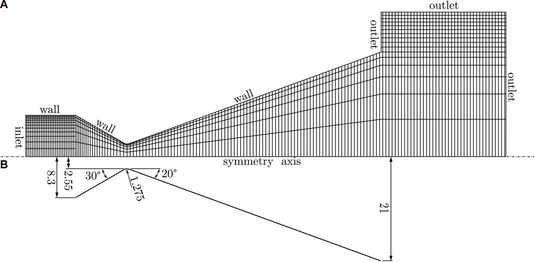
FIGURE 2. Rothe’s nozzle geometry (B) and numerical mesh (A) with applied upstream and downstream domains.

2.4 Reference case definitions and physical boundary conditions

The B = 590 case of Rothe is chosen for simulation because it provides a complete set of experimental results and has also been studied by Ivanov and Markelov (Ivanov et al., 1999). With the given throat radius r* = 2.55 mm, an experimental stagnation chamber pressure of p_in = 473.54 Pa is derived from (Rothe, 1971), while the given pressure ratio p_in/p_∞ = 310 leads to a background pressure of about p_∞ = 1.53 Pa. The experimental stagnation gas temperature is set to T_in = 300 K (Rothe, 1971; Ivanov et al., 1999; Arlemark et al., 2012).

For all present DSMC simulations, the Maxwellian velocity distributions at the entrance and exit of initialized test particles are based on the stagnation temperature T_in. At the walls a temperature of T_w = T_in is applied. Wall collisions are treated by full diffuse scattering of the test particles according to their Maxwellian velocity distribution, while the side planes of the mesh reflect the simulation particles in a specular manner. Binary collisions are modeled by the Larsen-Borgnakke variable hard sphere model (Borgnakke and Larsen, 1975; Bird, 1994). The number of equivalent simulation particles is set to at least seven test particles per cell throughout the nozzle.

In the numerical study, the present mass flow driven inflow model is validated and compared with a velocity driven inflow model based on Bird’s equilibrium state formulation. Thus, two sets of analytically and numerically derived boundary conditions are presented.

3 Analytical results for mass flow boundary conditions

3.1 Transsonic conservation equations

For the velocity driven inflow model, temperature, number density and inflow velocity are derived from analytical theory. When analyzing the change of physical quantities over the axial course of the described Laval nozzle, a relation between local velocity and local sound velocity is established, taking into account the conservation of total enthalpy and the definition of sound velocity. With equivalence of the total enthalpy at the nozzle inlet (in), the nozzle throat (*) and the nozzle outlet (out)

$h_{\text{in}}+\frac{u_{\text{in}}^2}{2}=h_{*}+\frac{u_{*}^2}{2}=h_{\text{out}}+\frac{u_{\text{out}}^2}{2}(7)$

and substitution of the enthalpy depending on the relation of the adiabatic exponent κ, the enthalpy h and the speed of sound,

$\begin{array}{ll}\hfill a& =\sqrt{\kappa \frac{p}{\rho }}=\sqrt{\kappa \left(h-e\right)}=\sqrt{\kappa \left(c_p-c_v\right)T}=\sqrt{\left(\kappa -1\right)c_{p}T}\hfill \\ \hfill & =\sqrt{\left(\kappa -1\right)\left(h-h_{\text{ref}}\right)}\hfill \end{array}(8)$

the described relation of velocity and sound velocity at the reference positions results corresponding to the speed of sound far away from the nozzle with u_∞ = 0:

$\begin{array}{ll}\hfill \underset{h_{\infty }-h_{\text{ref}}}{\underbrace{\frac{a_{\infty }^2}{\kappa -1}}}& =\underset{h-h_{\text{ref}}}{\underbrace{\frac{a^2}{\kappa -1}}}+\frac{u^2}{2}\hfill \\ \hfill & \Rightarrow \frac{a_{\infty }^2}{\kappa -1}=\underset{h_{\text{in}}-h_{\text{ref}}}{\underbrace{\frac{a_{\text{in}}^2}{\kappa -1}}}+\frac{u_{\text{in}}^2}{2}=\underset{h_{*}-h_{\text{ref}}}{\underbrace{\frac{a_{*}^2}{\kappa -1}}}+\underset{\frac{a_{*}^2}{2}}{\underbrace{\frac{u_{*}^2}{2}}}\hfill \\ \hfill & =\underset{h_{\text{out}}-h_{\text{ref}}}{\underbrace{\frac{a_{\text{out}}^2}{\kappa -1}}}+\frac{u_{\text{out}}^2}{2}\hfill \end{array}(9)$

accordingly, the relationship between the speed of sound at long range and the local speed of sound as a function of Mach number can be described as follows:

$\frac{a_{\infty }}{a}=\sqrt{1+\frac{\kappa -1}{2}\frac{u^2}{a^2}}=\sqrt{1+\frac{\kappa -1}{2}{\text{Ma}}^2}.(10)$

by means of this relation, the local Mach number at the nozzle inlet and outlet can be predicted as a function of the local sound velocity.

$a=\sqrt{\kappa \left(c_p-c_v\right)T}\Rightarrow \frac{T_{\infty }}{T}={\left(\frac{a_{\infty }}{a}\right)}^2=1+\frac{\kappa -1}{2}{\text{Ma}}^2(11)$

for thermodynamically ideal gases, isobaric and isochoric heat capacity c_p and c_v results in a direct relationship between the relation of the sound velocities and the corresponding temperature relation.

3.2 Isentropic mach number relations

In order to make more concrete statements about the local change of thermophysical state variables, pressure, density and temperature changes for thermodynamically ideal gases are related to each other as follows:

$\begin{array}{ll}\hfill T\sim \frac{p}{\rho }& \Rightarrow \ln \frac{T}{T_{\infty }}=\ln \frac{p}{p_{\infty }}-\ln \frac{\rho }{{\rho }_{\infty }}+C\hfill \\ \hfill & \Rightarrow \frac{dT}{T}=\frac{dp}{p}-\frac{d\rho }{\rho }.\hfill \end{array}(12)$

accordingly, it is known that for isentropic changes of state, as in the Laval nozzle, pressure and density changes are described for ideal gases with 1/T = (c_p − c_v)ρ/p in the power relation to each other described as follows:

$0=\ln \frac{p}{p_{\infty }}-\frac{c_p}{c_v}\ln \frac{\rho }{{\rho }_{\infty }}=\ln \frac{p}{{\rho }^{\kappa }}\Rightarrow p\sim {\rho }^{\kappa }.(13)$

for thermodynamically ideal gases, the corresponding relation to the temperature change follows:

$p\sim \rho T\Rightarrow T\sim \frac{p}{\rho }\sim {\rho }^{\kappa -1}\sim p^{\frac{\kappa -1}{\kappa }}.(14)$

hereby, over the entire course of the investigated nozzle, the temperature and density changes result from the axial pressure change depending on the corresponding temperature relation (Eq. 11). With the general equations

$\frac{{\rho }_{\infty }}{\rho }={\left(\frac{T_{\infty }}{T}\right)}^{\frac{1}{\kappa -1}}={\left(1+\frac{\kappa -1}{2}{\text{Ma}}^2\right)}^{\frac{1}{\kappa -1}}(15)$

$\frac{p_{\infty }}{p}={\left(\frac{T_{\infty }}{T}\right)}^{\frac{\kappa }{\kappa -1}}={\left(1+\frac{\kappa -1}{2}{\text{Ma}}^2\right)}^{\frac{\kappa }{\kappa -1}}(16)$

the relative density and pressure change is determined.

3.3 Specific relations of laval nozzle

In order to be able to make reliable statements regarding the velocity change within the nozzle with varying cross-sectional areas in the axial direction, velocity and density relations must be substituted on the basis of mass conservation as follows:

$\begin{array}{ll}\hfill \rho uA& ={\rho }_{*}{a}_{*}{A}_{*}\hfill \\ \hfill & \Rightarrow \frac{A}{A_{*}}=\frac{{\rho }_{*}{a}_{*}}{\rho u}=\frac{1}{\text{Ma}}\frac{{\rho }_{*}{a}_{*}}{\rho a}\hfill \\ \hfill & =\frac{1}{\text{Ma}}\frac{{\rho }_{*}}{{\rho }_{\infty }}\frac{{\rho }_{\infty }}{\rho }\frac{a_{*}}{a_{\infty }}\frac{a_{\infty }}{a}.\hfill \end{array}(17)$

from the homogeneity of the total enthalpy, the desired relations result for the local changes of sound velocity

$\frac{a_{\infty }^2}{\kappa -1}=\frac{a_{*}^2}{\kappa -1}+\frac{a_{*}^2}{2}=\frac{\kappa +1}{2\left(\kappa -1\right)}{a}_{*}^2\Rightarrow \frac{a_{*}}{a_{\infty }}=\sqrt{\frac{2}{\kappa +1}}(18)$

and density following the developped relations:

$\frac{{\rho }_{*}}{{\rho }_{\infty }}={\left(\frac{T_{*}}{T_{\infty }}\right)}^{\frac{1}{\kappa -1}}={\left(\frac{a_{*}}{a_{\infty }}\right)}^{\frac{2}{\kappa -1}}={\left(\frac{2}{\kappa +1}\right)}^{\frac{1}{\kappa -1}}.(19)$

After appropriate substitution of the nozzle-throat specific relations (Eqs 18, 19) and the general transsonic relations (Eqs 10, 15) to the mass conservation (Eq. 17), the final equation for the local Mach number,

$\begin{array}{ll}\hfill \frac{A}{A_{*}}& =\frac{1}{\text{Ma}}\underset{{\left(\frac{2}{\kappa +1}\right)}^{\frac{1}{\kappa -1}}}{\underbrace{\frac{{\rho }_{\ast }}{{\rho }_{\infty }}}}\stackrel{{\left(1+\frac{\kappa -1}{2}{\text{Ma}}^2\right)}^{\frac{1}{\kappa -1}}}{\overbrace{\frac{{\rho }_{\infty }}{\rho }}}\underset{\sqrt{\frac{2}{\kappa +1}}}{\underbrace{\frac{a_{\ast }}{a_{\infty }}}}\stackrel{\sqrt{1+\frac{\kappa -1}{2}{\text{Ma}}^2}}{\overbrace{\frac{a_{\infty }}{a}}}\hfill \\ \hfill & =\frac{1}{\text{Ma}}{\left(\frac{2}{\kappa +1}\left(1+\frac{\kappa -1}{2}{\text{Ma}}^2\right)\right)}^{\frac{\kappa +1}{2\left(\kappa -1\right)}}\hfill \end{array}(20)$

which can only be solved implicitly, is obtained as a function of the ratio of the local cross-sectional area to that at the nozzle throat.

3.4 Algorithm determining mach numbers on domain boundaries

By understanding one of the two positions in the equation as an iteration step of the Mach number, two iteration rules result for all permutations of iteration steps k and k + 1. The first one serves for the development of the Mach number Ma_in < 1 at the nozzle inlet with A = A_in in Eq. 20 as follows:

$\begin{array}{ccc}\hfill & \hfill & \frac{A_{\text{in}}}{A_{*}}=\frac{1}{{\text{Ma}}_{\text{in}}^{\left(k+1\right)}}{\left(\frac{2}{\kappa +1}\left(1+\frac{\kappa -1}{2}{\left({\text{Ma}}_{\text{in}}^{\left(k\right)}\right)}^2\right)\right)}^{\frac{\kappa +1}{2\left(\kappa -1\right)}}\hfill \\ \hfill & \hfill & \Rightarrow {\text{Ma}}_{\text{in}}^{\left(k+1\right)}=\frac{A_{*}}{A_{\text{in}}}{\left(\frac{2}{\kappa +1}\left(1+\frac{\kappa -1}{2}{\left({\text{Ma}}_{\text{in}}^{\left(k\right)}\right)}^2\right)\right)}^{\frac{2\left(\kappa -1\right)}{\kappa +1}}.\hfill \end{array}(21)$

The second iteration rule results from the alternative form of resolution according to the nozzle outlet with A = A_out as follows:

$\begin{array}{c}\frac{A_{\text{out}}}{A_{*}}=\frac{1}{{\text{Ma}}_{\text{out}}^{\left(k\right)}}{\left(\frac{2}{\kappa +1}\left(1+\frac{\kappa -1}{2}{\left({\text{Ma}}_{\text{out}}^{\left(k+1\right)}\right)}^2\right)\right)}^{\frac{\kappa +1}{2\left(\kappa -1\right)}}\hfill \\ \Rightarrow {\text{Ma}}_{\text{out}}^{\left(k+1\right)}=\sqrt{\frac{2}{\kappa -1}\left(\frac{\kappa +1}{2}{\left({\text{Ma}}_{\text{out}}^{\left(k\right)}\frac{A_{\text{out}}}{A_{*}}\right)}^{2\frac{\kappa -1}{\kappa +1}}-1\right)}.\hfill \end{array}(22)$

The result corresponds to the Mach number at the outlet of the nozzle Ma_out > 1. With a nozzle inlet diameter of 16.6 mm, a nozzle throat diameter of 5.1 mm, and a nozzle outlet diameter of 42.0 mm, the following Mach numbers result with the adiabatic exponent κ = 1.4 at the inlet and outlet:

${\text{Ma}}_{\text{in}}=0.05472(23)$

${\text{Ma}}_{\text{out}}=6.48801.(24)$

both iteration cycles start with Ma⁽⁰⁾ = 1. The inlet velocity u_in = 19.31 m/s results from the sound velocity a_in = 353.07 m/s at the inlet temperature T_in = 300 K.

Ivanov and Markedov (Ivanov et al., 1999) reported that no difference in flow properties is observed in the respective nozzle geometry whether simulation particles are inserted with a radially constant velocity profile or with a physically more correct parabolic velocity profile when using an inlet domain of the given size as in Figure 2. Therefore, in the present study, test particles with a radially uniform velocity are inserted on the left side of the inlet domain, as described by Arlemark et al. (Arlemark et al., 2012).

3.5 Mass flow modeling

In contrast to the velocity driven inflow, the boundary conditions for the present inflow model must be set differently. Using Eq. 2, the number of initialized test particles per time step is derived from the mass flow rate, the molecule mass and the area of the inlet. Since Rothe does not give mass flow rates in his studies (Rothe, 1971), the inlet number flux ${\dot{N}}_{\text{in}}$ is derived indirectly from the mass flow rate results of two simulations by Ivanov and Markedov (Ivanov et al., 1999) and the received mass flow rate of our own simulation using the velocity driven inflow model. The number density n_in at the inlet is calculated from the steady-state pressure equation

$p=n{k}_{B}T,(25)$

with the given values for stagnation pressure p_in and temperature T_in and the Boltzmann constant k_B. The mass flow rate $\dot{m}$ at the inlet may be calculated using

${\rho }_{\text{in}}=n_{\text{in}}m,(26)$

for the stagnation density ρ_in and

${\dot{m}}_{\text{in}}={\rho }_{\text{in}}{u}_{\text{in}}{A}_{\text{in}}.(27)$

The vacuum condition at the velocity driven outflow is modeled using the inlet number density value, but with a high flow velocity out of the outlet region. Exceptionally the value has to be larger than the ratio of normal cell length and time step. Assuming that the exit temperature in the diffuser is not greater than the entrance temperature, the exit velocity should not be greater than the product of the expected Mach number at the exit Ma_out (Eq. 24) and the speed of sound at the entrance a_in = 353.07 m/s, so as not to disturb the display in postprocessing. The product of the two actual values would be approx. 2,290 m/s. For the velocity driven simulations, the outlet velocity is set to u_out = 2000 m/s for each of the three outlet surfaces in Figure 2.

Thus, the results for the present inflow model are indicated by the notation A, B, or C. Case A uses the numerical mass flow rate from the GASP solver (AeroSoft, Inc., 1996), while case B uses the mass flow rate from the SMILE solver (Ivanov et al., 1999), both values presented by Ivanov and Markedov in (Ivanov et al., 1999) for the B = 590 test case. For case C, on the other hand, the mass flow rate is calculated from own DSMC simulations, performed with basically the same solver, but with the velocity driven inflow model, using Eq. 27. For a better understanding, the validation process for the present study is shown in Figure 3. The outlet boundary number density is set using Eq. 25 according to the background pressure p_∞ of Rothe’s experiments. Additionally, the macroscopic flow velocity at the outlet is set as described for the velocity driven inflow model. An overview of the used boundary conditions is given in Table 1.

FIGURE 3

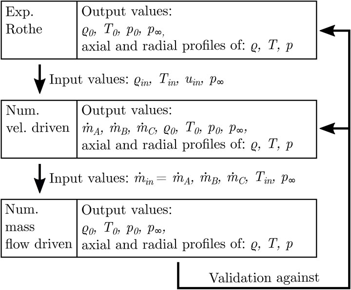
FIGURE 3. In- and Output values for the validation process.

TABLE 1

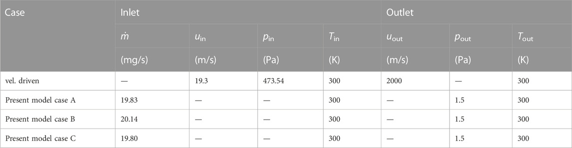
TABLE 1. Overview of in- and outlet boundary conditions for the present study.

4 Discussion of simulation data with modelled conditions

4.1 Centerline and radial temperature profiles

Experimental and numerical results of the rotational temperature for the B = 590 case of the Rothe nozzle are shown in Figure 4. The temperatures of all data are scaled by the experimental stagnation chamber temperature T_in = 300 K. On the left side of Figure 4 are centerline temperatures of Rothe’s experiment, numerical results for GASP and SMILE solvers, and results of four corresponding simulations using the present and the velocity driven inflow models. The radial position is scaled by the throat radius r*, where zero indicates the position of the nozzle throat.

FIGURE 4

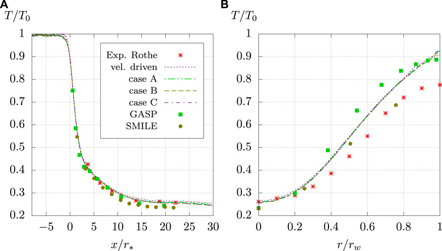
FIGURE 4. Centerline (A) and radial (B) rotational temperature profiles for Rothe’s nozzle. Experimental results from (Rothe, 1971), numerical results for GASP and SMILE obtained from (Ivanov et al., 1999).

All solvers reproduce the experimental stagnation temperature of 300 K well, with only small numerical scatter in the results. Deviations begin to occur downstream of the nozzle throat with decreasing temperatures. While the first points of the GASP and SMILE results agree well with the present results, the deviations increase near the nozzle exit, which is at about x/r* = 20.

The DSMC solver SMILE reproduces the lowest rotational temperatures compared to the other solvers. While in a single comparison with the Navier-Stokes solver GASP, differences can be explained by the use of no-slip wall boundary conditions for the GASP code (Ivanov et al., 1999), which probably results in higher core flow velocities for the DSMC code and therefore lower rotational temperatures in the nozzle axis, the deviations compared to the results obtained in this paper cannot be explained by this. For the diffuser part of the nozzle, with x/r* > 0, it can be seen that the rotational temperatures predicted by the present simulations agree very well with the experimental data of Rothe. After the nozzle exit plane, the temperature curves of the present simulations drop slightly due to expansion effects of the applied vacuum boundary conditions.

The radial temperature profiles are shown on the right in Figure 4. The axial position of the profiles is near the nozzle exit at x/r* = 18.7. The radial position of the temperature is scaled by the local nozzle radius r_w. Deviations from experimental data are present in all simulations. The DSMC solver SMILE underpredicts temperature values near the centerline, but reproduces the experimental temperature profile quite well. All other solvers show large deviations near the nozzle wall. In particular, in the present simulations, the solvers do not reproduce the correct temperature values for almost 80% of the nozzle radius, and the temperature profile is lifted above the experimental results. This effect is not unexpected and is explained by the treatment of the temperature boundary conditions at the wall, which are calculated to be T_w = T_in. This behavior was also observed by Arlemark et al. in their study (Arlemark et al., 2012).

For both axial and radial temperature profiles, no major deviations are observed, which could be traced back to the three and slightly different mass flow rates of cases A, B and C used in the present simulations.

4.2 Centerline and radial mass density

A comparison of the axial and radial mass density profiles for the discussed solvers is shown in Figure 5. The axial density profiles on the left side of the figure are scaled by the stagnation chamber density ρ_in from Rothe’s experiment, while the axial position is scaled by the throat radius r*. For better comparison the values are logarithmic.

FIGURE 5

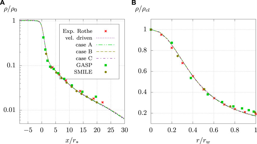
FIGURE 5. Centerline (A) and radial (B) density profiles for Rothe’s nozzle. Experimental results from (Rothe, 1971), numerical results for GASP and SMILE obtained from (Ivanov et al., 1999).

All present simulations reproduce well the centerline density for the pressurized part of the nozzle. There is only a small overprediction of the centerline density. The deviations scale from about 1% to 4% depending on the mass flow rate used for cases A, B, and C. The smallest deviation of 1% is present for case C, which has the lowest mass flow rate. Deviations from the experimental results appear again in the second half of the diffuser. Here, the Navier-Stokes solver GASP overpredicts the experimental data, while all DSMC solvers tend to underpredict the centerline density. Deviations from experimental values can reach 10%, although this value can only be given for the present simulations. Behind the nozzle exit at about x/r* = 20, the mass density continues to decrease due to the suction effects of the applied boundary conditions and the expansion of the flow.

Radial mass density profiles for x/r* = 18.7 are shown in the right part of Figure 5. The mass density is scaled by the centerline value ρ_cl and the radial position is scaled by the nozzle radius at the given position. It can be seen that all solvers reproduce the density very well with only small deviations, while the DSMC results are slightly closer to the experimental ones.

4.3 Centerline pressure distribution

Centerline pressure profiles for the B = 590 case of the Rothe nozzle are shown in Figure 6. All results are scaled by the stagnation pressure p_in from the experiment and plotted logarithmically. The axial direction is again scaled by the nozzle throat radius r*. While the pressure values for the present simulations are obtained directly, they have to be derived from the mass density and temperature for GASP, SMILE and experimental data.

FIGURE 6

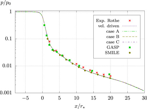
FIGURE 6. Centreline pressure profiles for Rothe’s nozzle. Experimental results from (Rothe, 1971), numerical results for GASP and SMILE derived from (Ivanov et al., 1999).

It can be seen that the present simulations reproduce the centerline pressure very well for the pressurized part of the Rothe nozzle. Deviations from experimental data range from 0.5% to 2%. In the diffuser part of the nozzle there are deviations from the experimental data. The Navier-Stokes code GASP reproduces the centerline pressure profile best, with only a small overprediction for the last displayed value. The overprediction at the nozzle exit may be due to the fact that for the GASP simulations in the study by Ivanov et al. (Ivanov et al., 1999), the outlet patch is applied directly to the nozzle exit plane and therefore the numerical deviation is observed. Unfortunately, the good agreement with the experimental values is achieved by underpredicting the temperature and overpredicting the density, see the left sides of Figures 4, 5.

For all DSMC solvers, a slight underprediction of the experimental pressure can be seen in Figure 6. For the present simulations, it can be seen that the deviation is caused by an underprediction of the centerline density, since the centerline temperature values are in excellent agreement with the experimental data. For the DSMC code SMILE, the underprediction of the experimental centerline pressure can be caused by an underprediction of both temperature and density, as seen in Figures 4, 5.

5 Conclusion

A mass flow driven inflow model for the DSMC method is described and presented. In the model, the inflow is derived from the experimental mass flow rate, geometric dimensions, and molecular properties of the gas used. The inflow model was validated using the well-known B = 590 experimental test case from Rothe’s nozzle study, as well as numerical results from a second study by Ivanov and Markelov.

The comparison of the rotational centerline temperature was in excellent agreement with the experimental and numerical results, reproducing well the stagnation temperature and the temperature drop along the nozzle axis. Radial profiles of rotational temperatures at the nozzle exit, near the nozzle wall, were higher than the experimental ones due to the applied boundary conditions.

The centerline density distribution was also in good agreement with the experimental and numerical results, reproducing the stagnation density well with only small deviations between 1% and 4%. The prediction of the radial density distribution at the nozzle exit was also in good agreement with the experimental values.

The numerical pressure distribution along the nozzle axis resulting from the obtained temperature and density was in good agreement with the distributions from the other studies and reproduced the experimental stagnation of the case very well with deviations between 0.5% and 2%.

It is shown that when the proposed mass flow driven inflow model is applied to the Rothe nozzle test case, the results are in good agreement, validating the approach. The presented inflow model is particularly suitable for arbitrary nozzle flow cases with higher density subsonic inflow conditions. The inflow mass flow rate and temperature, as well as the vacuum background pressure, need to be known only from the experiment in order to apply the model. Since the approach is based on the mass flow rate, the calculation of the inflow velocity from the analytical 1D de Laval theory may be obsolete, thus potentially eliminating possible sources of error resulting from theory-based calculations.

Data availability statement

The original contributions presented in the study are included in the article/Supplementary material, further inquiries can be directed to the corresponding author.

Author contributions

RG and TF contributed to conception and design of the study. RG performed the analytical analysis. TF performed the numerical computation. RG and TF wrote the first draft of the manuscript. RG and TF wrote sections of the manuscript. All authors contributed to the article and approved the submitted version.

Funding

The authors would like to thank the “North-German Supercomputing Alliance” (HLRN) for providing the computational time for the numerical study in this work (Funding ID: hbi00027).

Conflict of interest

The authors declare that the research was conducted in the absence of any commercial or financial relationships that could be construed as a potential conflict of interest.

Publisher’s note

All claims expressed in this article are solely those of the authors and do not necessarily represent those of their affiliated organizations, or those of the publisher, the editors and the reviewers. Any product that may be evaluated in this article, or claim that may be made by its manufacturer, is not guaranteed or endorsed by the publisher.

References

AeroSoft, Inc. (1996). Gasp version 3 user’s manual. Blacksburg, Virginia.

Google Scholar

Akhlaghi, H., and Roohi, E. (2014). Mass flow rate prediction of pressure-temperature-driven gas flows through micro/nanoscale channels. Continuum Mech. Thermodyn. 26, 67–78. doi:10.1007/s00161-013-0290-0

CrossRef Full Text | Google Scholar

Alexeenko, A., Levin, D., Gimelshein, S., Collins, R., and Reed, B. (2002). Numerical modeling of axisymmetric and three-dimensional flows in microelectromechanical systems nozzles. AIAA J. 40, 897–904. doi:10.2514/2.1726

CrossRef Full Text | Google Scholar

Arlemark, E., Markelov, G., and Nedea, S. (2012). Rebuilding of Rothe’s nozzle measurements with OpenFOAM software. J. Phys. Conf. Ser. 362, 012040. doi:10.1088/1742-6596/362/1/012040

CrossRef Full Text | Google Scholar

Bird, G. (1970). Direct simulation and the Boltzmann equation. Phys. Fluids 13, 2676–2681. doi:10.1063/1.1692849

CrossRef Full Text | Google Scholar

Bird, G. A. (1994). Molecular gas dynamics and the direct simulation of gas flows.

Google Scholar

Bird, G. (2007). “Sophisticated dsmc,” in Notes prepared for a short course at the DSMC07 meeting, Santa Fe, USA.

Google Scholar

Borgnakke, C., and Larsen, P. (1975). Statistical collision model for Monte Carlo simulation of polyatomic gas mixture. J. Comput. Phys. 18, 405–420. doi:10.1016/0021-9991(75)90094-7

CrossRef Full Text | Google Scholar

Chung, C.-H., Kim, S. C., Stubbs, R. M., and De Witt, K. J. (1995). Low-density nozzle flow by the direct simulation Monte Carlo and continuum methods. J. Propuls. Power 11, 64–70. doi:10.2514/3.23841

CrossRef Full Text | Google Scholar

Darbandi, M., and Roohi, E. (2011). Study of subsonic–supersonic gas flow through micro/nanoscale nozzles using unstructured DSMC solver. Microfluid. Nanofluidics 10, 321–335. doi:10.1007/s10404-010-0671-7

CrossRef Full Text | Google Scholar

Fang, Y., and Liou, W. (2002). Computations of the flow and heat transfer in microdevices using dsmc with implicit boundary conditions. ASME. J. Heat. Transf. 124, 338–345. doi:10.1115/1.1447933

CrossRef Full Text | Google Scholar

Farbar, E., and Boyd, I. (2014). Subsonic flow boundary conditions for the direct simulation Monte Carlo method. Comput. Fluids 102, 99–110. doi:10.1016/j.compfluid.2014.06.025

CrossRef Full Text | Google Scholar

Frieler, T., and Groll, R. (2023). Micro-nozzle flow and thrust prediction with high density ratio using DSMC selection limiter. Front. Space Technol. 4. doi:10.3389/frspt.2023.1114188

CrossRef Full Text | Google Scholar

Ivanov, S., Markelov, N., Kashkovsky, V., and Giordano, D. (1997). “Numerical analysis of thruster plume interaction problems,” in European Spacecraft Propulsion Conference, 603.

Google Scholar

Ivanov, M., Markelov, G., Ketsdever, A., and Wadsworth, D. (1999). Numerical study of cold gas micronozzle flows. AIAA paper, 11.

Google Scholar

Kim, S. (1994). Calculations of low-Reynolds-number resistojet nozzles. J. Spacecr. Rockets 31, 259–264. doi:10.2514/3.26431

CrossRef Full Text | Google Scholar

Kühn, C., and Groll, R. (2021). picfoam: An openfoam based electrostatic particle-in-cell solver. Comput. Phys. Commun. 262, 107853. doi:10.1016/j.cpc.2021.107853

CrossRef Full Text | Google Scholar

Lei, M., Wu, X., Zhang, W., Li, X., and Chen, X. (2017). The implementation of subsonic boundary conditions for the direct simulation Monte Carlo method in dsmcfoam. Comput. Fluids 156, 209–219. doi:10.1016/j.compfluid.2017.07.010

CrossRef Full Text | Google Scholar

Liou, W., and Fang, Y. (2000). Implicit boundary conditions for direct simulation Monte Carlo method in mems flow predictions. Model. Eng. Sci. 1, 119–128. doi:10.3970/cmes.2000.001.571

CrossRef Full Text | Google Scholar

Liu, M., Zhang, X., Zhang, G., and Chen, Y. (2006). Study on micronozzle flow and propulsion performance using DSMC and continuum methods. Acta Mech. Sin. 22, 409–416. doi:10.1007/s10409-006-0020-y

CrossRef Full Text | Google Scholar

Nance, R. P., Hash, D. B., and Hassan, H. A. (1997). Role of boundary conditions in Monte Carlo simulation of microelectromechanical systems. J. Thermophys. Heat Transf. 12, 447–449. doi:10.2514/2.6358

CrossRef Full Text | Google Scholar

OpenFOAM Ltd (2016). OpenFOAM: The open source CFD toolbox, user guide.

Google Scholar

Plotnikov, M. Y., and Shkarupa, E. V. (2021). Two approaches to calculating composition of rarefied gas mixture exposed to chemical reactions at flow through cylindrical channel. Comput. Fluids 214, 104775. doi:10.1016/j.compfluid.2020.104775

CrossRef Full Text | Google Scholar

Roohi, E., Darbandi, M., and Mirjalili, V. (2009). Direct simulation Monte Carlo solution of subsonic flow through micro/nanoscale channels. J. heat Transf. 131, 092402. doi:10.1115/1.3139105

CrossRef Full Text | Google Scholar

Rothe, D. E. (1965). Flow visualization using a traversing electron beam. AIAA J. 3, 1945–1946. doi:10.2514/3.3286

CrossRef Full Text | Google Scholar

Rothe, D. E. (1971). Electron-beam studies of viscous flow in supersonic nozzles. AIAA J. 9, 804–811. doi:10.2514/3.6279

CrossRef Full Text | Google Scholar

Scanlon, T., Roohi, E., White, C., Darbandi, M., and Reese, J. (2010). An open source, parallel DSMC code for rarefied gas flows in arbitrary geometries. Comput. Fluids 39, 2078–2089. doi:10.1016/j.compfluid.2010.07.014

CrossRef Full Text | Google Scholar

Shang, Z., and Chen, S. (2013). 3D DSMC simulation of rarefied gas flows around a space crew capsule using OpenFOAM. Open J. Appl. Sci. 3, 35–38. doi:10.4236/ojapps.2013.31005

CrossRef Full Text | Google Scholar

Wang, M., and Li, Z. (2004). Simulations for gas flows in microgeometries using the direct simulation Monte Carlo method. Int. J. Heat Fluid Flow 25, 975–985. doi:10.1016/j.ijheatfluidflow.2004.02.024

CrossRef Full Text | Google Scholar

Zelesnik, D., Micci, M. M., and Long, L. N. (1994). Direct simulation Monte Carlo model of low Reynolds number nozzle flows. J. Propuls. Power 10, 546–553. doi:10.2514/3.23807

CrossRef Full Text | Google Scholar