Model-based performance study of an industrial single spool gas turbine 9EA-GT by changing the inlet guide vane angle and modifying the compressor map

1 Introduction

One of the most important components of contemporary technology, gas turbines (GTs) are the primary mechanical power sources for large pumps and turbines as well as the aviation and energy sectors (Talaat et al., 2018). GTEs are widely used in the factory and aeronautical sectors. In industrial workplaces, these are often used to provide mechanical energy for various loads, including massive pumps and compressors, tanks, ships, and other transport vehicles, as well as for powering generators that create electricity. In electricity generation plants, GTs may be used independently or in conjunction with a steam turbine, either in mixed cycles or in cogeneration, to provide both electrical energy and industrial heat processing (Talaat et al., 2019; Talaat et al., 2021; Talaat et al., 2022). To provide high efficacy, the mixed cycle plant, which is often utilized for energy production, is equipped with more than one GT and, frequently, one steam turbine (Cohen et al., 1987; Talaat et al., 2018).

A gas turbine engine (GTE) is an example of a thermodynamic device that efficiently completes its tasks within the parameters of the design. Air and gas (combustion byproducts) are used as operating fluids in the cold and hot portions, as the fuel and air are used to transform the fuel chemical energy into mechanical energy (Cohen et al., 1987; McBride et al., 2002; Talaat et al., 2018).

A gas turbine’s performance is influenced by several variables, some of which are impossible to regulate by external forces. Examples include elevated air temperatures and humidity levels, as well as pollutants in the environment. Additional variables that can be adjusted include turbine and compressor fouling, which can be fixed by washing these parts. Component deterioration is fixed by swapping out the damaged element (Cohen et al., 1987; Talaat et al., 2023).

The performance of industrial gas turbines deteriorates over time due to aging and bad environmental conditions. Considering both time and safety, it is important to predict the system’s health condition to plan a suitable maintenance policy. Fault diagnosis occurs through analysis of gas path parameters that can be measured during operation and should be detected using the deterioration detection system. Analyzing those measurements can determine the degradation of engine components. Often, the mathematical model is designed to generate the degradation database because of the difficulty in obtaining such data for the real engine (Ogaji et al., 2005; Razak, 2007; Morini et al., 2010; Roumeliotis, 2010; Ogbonnaya, 2011; Awang Saifudin and Mazlan, 2014; Talaat et al., 2018).

The GT design and off-design models discussed in this study seek to be computationally simple while also being able to handle plants with significant operational parameter variability. The estimation of machine off-design behavior is the main challenge in the creation of an off-design model (Asgari et al., 2013; Nikpey et al., 2013; SadoughVanini et al., 2014). The stage-stacking technique should be used to build the model, modeling the performance maps of each machine phase, and measurement data of each compressor and turbine phase should be used for verification (Cohen et al., 1987; McBride et al., 2002; Razak, 2007; Li et al., 2011; Palmé et al., 2011; Awang Saifudin and Mazlan, 2014; Talaat et al., 2018). There are generally no data on individual performance maps as manufacturers rarely give customers access to GT efficacy data, and a mathematical model is required to forecast machine performance (Cohen et al., 1987; Talaat et al., 2018; Talaat et al., 2023).

The factors mentioned above arise because of an engine running continuously. However, these events can be postponed by using higher-quality fuels, operating the engine safely, and performing routine maintenance. To address this problem, numerous researchers have constructed representative models of the deterioration influencing gas turbine performance using the laws of thermodynamics. Performance maps are applied to these thermodynamic models to represent the engine components. The degradation that results from changing the compressor and turbine performance is simulated by the performance maps. If there is deterioration in the engine components, the thermodynamic models are used to compute changes in the gas turbine performance. Researchers have suggested using artificial intelligence to identify and forecast a gas turbine’s deterioration (Talaat et al., 2023).

The two citations support this paragraph performance of a GT is influenced by several variables, including difficult-to-control external variables. Examples include air temperature and humidity as well as nearby environmental contamination. Compressor fouling and the turbine are other issues that may be rectified. These might be fixed by cleaning the affected parts. By swapping out the damaged component, erosion in the components is corrected (Razak, 2007; Morini et al., 2010; Awang Saifudin and Mazlan, 2014; Talaat et al., 2018).

The incidence of the variables is caused by an engine running continuously, but they may be prevented by operating an engine safely, using better fuel, and performing routine maintenance. Numerous authors have addressed this problem by creating models that depict a decline in GT efficiency using the laws of thermodynamics (Talaat et al., 2018). By using performance maps that replicate the degradation with variations in the compressor and turbine performance, these thermodynamic models are utilized to describe the engine parts (Ogaji et al., 2005; Roumeliotis, 2010; Talaat et al., 2018). Authors recommended using artificial intelligence to identify and then anticipate the degradation in a GT because thermodynamic models have been shown to quantify changes in GT performance if degradation occurs in engine parts (Liu et al., 2010a; Liu et al., 2010b; Liu and Cao, 2010; Farahat and Talaat, 2012; Talaat et al., 2018; Talaat et al., 2023; Tayseer et al., 2024).

The degradation variables cause the GT to deteriorate. Due to increased fuel usage, these variables cause high operating costs. The conflict between an investor’s goal and their environmental duty is encouraged by the energy market’s independence. The maintenance crews must be focused on detecting any signs of GT performance degradation wherever they may occur, as the fuel price is very high. The detection of deterioration becomes crucially important with a large increase in fuel cost in order to preserve the industrial GT’s health and optimal performance (Liu et al., 2010b). Due to the challenges of acquiring deteriorating datasets from the actual engine, mathematical models are frequently used to construct them. Then, using the database generated, the mathematical model will be utilized as the detecting tool to analyze the engine measurement data (Cohen et al., 1987; Liu et al., 2010b; Talaat et al., 2018).

Several degradation variables may impact how well a GT operates. Several of these elements do, however, have a discernible impact on GTs’ general performance. Combustion, compressor, turbine, air capacity, and air filter efficiency are a few of the factors for deterioration (Cohen et al., 1987; Liu et al., 2010b; Talaat et al., 2018). Other performance-degrading variables include guiding vanes that are misaligned, air and gas leaks, and problems with the intake and exhaust ducts. All GTEs will experience performance degradation throughout operation time due to deterioration factors. A GTE is susceptible to many physical problems, such as erosion, corrosion, fouling, built-up dirt, excessive tip, and foreign object damage. These problems cause degradations in the engine performance parameters (component efficiency and pumping capacity). This results in changes in the engine-measured parameters (pressures and temperatures), which are dependent. Engine monitoring techniques are used to determine health and, consequently, determine the suitable maintenance actions for the engine. This is done by inter-relating the change in the engine-measured parameters with the deterioration in the performance parameters.

When developing a turbine model, understanding how an engine’s changing technical state affects its operational characteristics is essential. The compressor is especially vulnerable to variations in the engine’s operating condition. Any disruptions in the system’s operation will result in changes in the compressor and engine operation similar to those brought on by varying rotational speed or clogged compressor blade passages if the compressor design includes a control system for adjusting the controllable blades of the guide vanes to optimize all the engine units by continuously correcting the compressor features.

In this study, generalized machine maps were acquired from previous studies, and fresh maps were created utilizing the correct scaling strategies for the GTs under consideration. The maps were then confirmed using experimental data obtained for the entire machine. In this article, the two models used in the calculations for steady-state performance were the steady-state behavior at engine startup (from 65% to 100% speed, without load) and steady-state behavior while loading (constant speed of 100%). This model addresses the difficulties caused by the lack of understanding of stage-by-stage performance by using appropriate scaling techniques to create artificial machine maps based on generalized maps derived from prior research and verifying them with experimental observations from actual power plants.

2 Mathematical model

When simulating an engine, mathematical models provide insights into its features. The compressor, combustor, and turbine are the three primary parts of a GTE, which together define its total performance. The simple models of a turbine engine, see Figure 1, and turbine maps are extracted from a high-level GT simulation program.

Figure 1

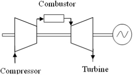
Figure 1. GT flow sheet model.

A single-shaft GT that produces electricity is the thermal system that will be modeled (single spool 9EA GASTURBINE); see Table 1. An open Brayton–Joule cycle devoid of regeneration serves as the benchmark thermodynamic cycle; see Figure 1. It was created as a model to forecast plant static performance in both on- and off-design situations. The model considers the impact of varying inlet guide vanes (VIGVs) on compressor efficiency. The model’s equations represent the mass or energy balances of its constituent parts. The model determines the flow rate, temperature, and pressure at each location in the system.

Table 1

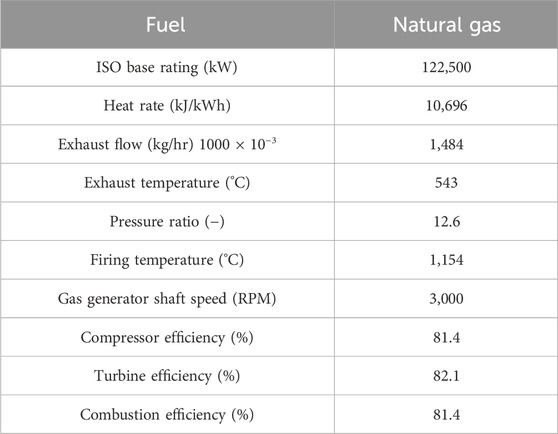
Table 1. 9EA-GT design variables.

2.1 Component map scaling

The component maps serve as the foundation for the functioning of the main engine parts. Equipment feature maps are private information that is typically challenging to obtain from GT suppliers. In most cases, analytical techniques are used to create these maps; see Figure 2.

Figure 2

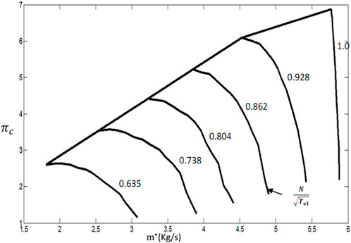
Figure 2. Axial compressor map before scaling.

To solve this issue, component maps for a different compressor and turbine are downloaded from the GasTurb 12 tool (Walsh and Fletcher, 1998; Najmi and Arhosazani, 2006) and scaled to the compressor and turbine’s design points for the investigated GTE. The traditional scaling approach produces scaled component maps by applying scaling factors obtained at the on-design location to the actual component maps at off-design locations; see Figure 3.

Figure 3

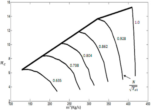
Figure 3. Axial compressor map after scaling.

Performance prediction of gas turbines is strongly dependent on a detailed understanding of the engine component behavior. Compressors are of special interest because they can generate many types of operability problems like surge, stall, and flutter; their operating line is determined by the turbine characteristics. Due to the unavailability of the actual component maps, the alternative maps are obtained from GasTurb 12 software, and appropriate adjustments are made using the scaling law in the software. In other words, after choosing the map-design point, the steady start model (discussed in detail in the following section) should be run to ensure that the starting operating line (the inclined part of the operating line) does not intersect with the surge line. If it does, the map-design point should be moved away from the maximum efficiency contour until the operating line is completely clear of the surge line. Both the studied compressor and turbine maps are predicted using theoretical maps and Eqs (1)–(3). Figures 2, 3 illustrate the compressor map before (old) and after (new) scaling, respectively.

${\mathrm{PR}}_{\text{model}}=\left[\frac{{\mathrm{PR}}_{\text{design}-\text{model}}-1}{{\mathrm{PR}}_{\text{design}-\text{map}}-1}\right]*\left({\mathrm{PR}}_{\text{map}}-1\right),(1)$

${\mathrm{m}}_{\text{model}}^{•}=\left[\frac{{\mathrm{m}}_{\text{design}\text{model}}^{•}}{{\mathrm{m}}_{\text{design}\text{map}}^{•}}\right]*\left({\mathrm{m}}_{\text{map}}^{•}\right),(2)$

${\mathrm{\eta }}_{\text{model}}=\left[\frac{{\mathrm{\eta }}_{\text{design}\text{model}}}{{\mathrm{\eta }}_{\text{design}\text{map}}}\right]*\left({\mathrm{\eta }}_{\text{map}}\right).(3)$

2.2 Compressor maps for various IGV angles

Knowing the impact of an engine’s variable technical status on its operating characteristics is a crucial issue when building a turbine model. A compressor is particularly sensitive to changes in the engine’s technical status while it is running. If the compressor design includes a control system for adjusting the guide vanes’ controllable blades to optimize all the engine units by continuously correcting the compressor features map, then any disruptions in the system’s operation will cause changes in the compressor and engine operation that are similar to those caused by varying rotational speed or clogged compressor blade passages. By adjusting the setting angles of the guide blade vanes while the compressor’s angular velocity is changing, implementing the inlet guide vane’s controllable blades of the specific compressor’s stages allows concurrently changing the inlet flow angles onto the blades of the rotor rings of the stages (Talaat et al., 2018; Song et al., 2023).

To modify the compressor maps for the steady-state model, we can study the changes for all parameters of the compressor map ($m^{•},\pi ,\eta$) for any change in IGV angle. The first step changes the mass flow rate. The mass flow rate can be represented by the following equation:

${\mathrm{m}}^{•}=\text{ca}*\mathrm{\rho }*\mathrm{A},(4)$

where $ca$ is axial velocity, $\rho$ is fluid density, and A is cross-section area.

The cross-section area properties are constant at any change of IGV angle, and the fluid density is assumed to be constant. From the previous assumptions, the mass flow rate depends on the axial velocity, which is as follows:

$\frac{{\mathrm{m}}_1^{•}}{{\mathrm{m}}_2^{•}}=\frac{{\text{ca}}_1}{{\text{ca}}_2}.(5)$

Figure 4 shows the relationship between IGV angle and axial velocity. From the velocity triangle at the inlet to the first rotor of the compressor, the axial velocity is a function of blade speed. The absolute and relative angles have a relationship between the IGV angle and the axial velocity:

$U=\frac{C_a}{\mathit{tan}\alpha }+\frac{C_a}{\mathit{tan}\beta },(\mathrm{6a})$

${Ca}_1=\frac{\mathrm{U}\mathit{tan}\alpha *\tan \mathrm{\beta }}{\mathit{tan}\alpha +\tan \mathrm{\beta }},(\mathrm{6b})$

where β is the blade angle.

Figure 4

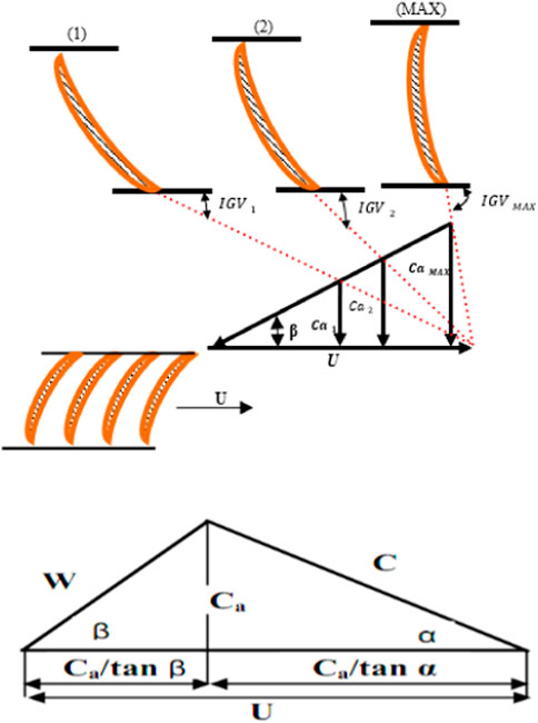
Figure 4. Control of compressor axial velocity by changing the IGV angle.

By substituting Eq. 6a, 6b into Eq. 5, the relationship between ${\mathrm{m}}^{•}$ and the IGV angle is given by

$\frac{{\mathrm{m}}_1^{•}}{{\mathrm{m}}_2^{•}}=\frac{\tan \text{IGV}1}{\tan \text{IGV}1+\tan \mathrm{\beta }}*\frac{\tan \text{IGV}2+\tan \mathrm{\beta }}{\tan \text{IGV}2}(7)$

The compressor map represented in Figure 5 is at the IGV fully open position, so the mass flow in the compressor map at any IGV angle position can be modified as follows.

${\mathrm{M}}_{\text{IGV}1}^{•}={\mathrm{m}}_{\text{IGV}\mathrm{F}.\mathrm{O}}^{•}\times \left[\frac{\tan \text{IGV}1}{\tan \text{IGV}1+\tan \mathrm{\beta }}\times \frac{\tan \text{IGV}\mathrm{F}.\mathrm{O}+\tan \mathrm{\beta }}{\tan \text{IGV}\mathrm{F}.\mathrm{O}}\right](8)$

Figure 5

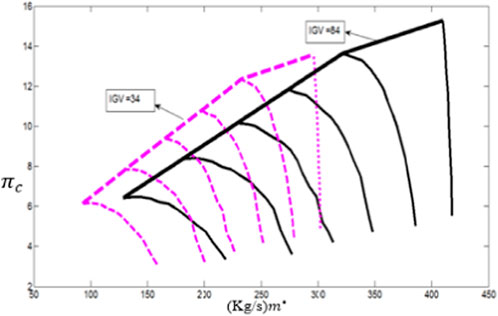
Figure 5. Compressor maps under variation of the IGV angle.

The next step modifies the pressure ratio and the efficiency in the compressor map. To do this, it is necessary to obtain the relationship between the pressure ratio and efficiency with the IGVs and all parameters in the compressor map.

$\mathit{PR}=f\left(IGV,m^{•},N\right)(9)$

$\eta =f\left(IGV,m^{•},N\right)(10)$

The overall relationship between the pressure ratio and efficiency is searched for using the set of regression equations (Meng et al., 2023; Meng et al., 2024a; Meng et al., 2024b) that approximate its universal characteristics.

The relationship between pressure ratio and efficiency is examined using a collection of regression models that simulate its universal properties.

${\mathit{PR}}_c=a_0+a_1{m}^{•}+a_2{\left[m^{•}\right]}^2+a_{3}N+a_4{\left[N\right]}^2+a_5{m}^{•}N+a_{6}IGV+a_7{\left[IGV\right]}^2+a_8{\mathrm{m}}^{•}\text{IGV}+a_{9}N*\text{IGV},(11)$

${ɳ}_c=b_0+b_1{\mathrm{m}}^{•}+b_2{\left[{\mathrm{m}}^{•}\right]}^2+b_{3}N+b_4{\left[N\right]}^2+b_5{\mathrm{m}}^{•}N+b_6\text{IGV}+b_7{\left[IGV\right]}^2+b_8{\mathrm{m}}^{•}\text{IGV}+b_{9}V*\text{IGV}.(12)$

Regression coefficients ai and bi are determined using real values from the 9EA-GT IGV system to obtain 10 equations with 10 unknowns. These equations are solved to obtain the coefficients ai and bi; see Table 2.

Table 2

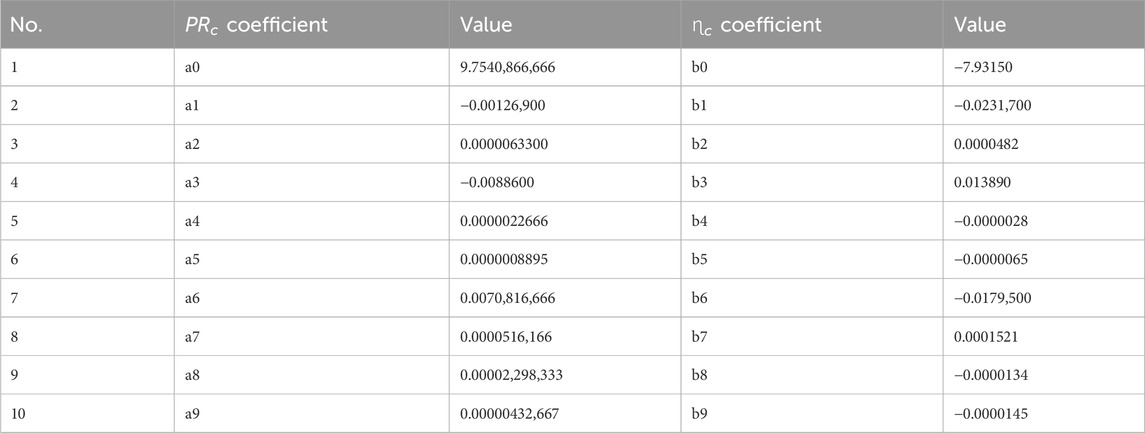
Table 2. Regression coefficients ai and bi.

To modify the pressure ratio and efficiency in the compressor map at any IGV angle position,

${\mathit{PR}}_{\text{IGV}1}={\mathit{PR}}_{\text{IGV}\mathrm{F}.\mathrm{O}}*\left[\frac{a_0+a_1{\mathrm{m}}_{\text{IGV}1}^{•}+\dots .+a_{9}N*\text{IGV}1}{a_0+a_1{\mathrm{m}}_{\text{IGV}\mathrm{F}.\mathrm{O}}^{•}+\dots .+a_{9}N*\text{IGV}\mathrm{F}.\mathrm{O}}\right],(13)$

${ɳ}_{\text{IGV}1}={ɳ}_{\text{IGV}\mathrm{F}.\mathrm{O}}*\left[\frac{b_0+b_1{\mathrm{m}}_{\text{IGV}1}^{•}+\dots .+b_{9}N*\text{IGV}1}{b_0+b_1{\mathrm{m}}_{\text{IGV}\mathrm{F}.\mathrm{O}}^{•}+\dots .+b_{9}N*\text{IGV}\mathrm{F}.\mathrm{O}}\right].(14)$

2.3 Thermodynamic process concepts

GTs generate electricity by transforming heat into work. The heat intake is the result of igniting the fuel in the combustor. Because of this, the use of thermodynamic laws is the best way to analyze GT efficiency. The thermodynamic parameters of the working medium, which include the enthalpy, entropy, gas constant, and specific heat at constant pressure, must be determined at every point along the passage of gases. The following relationships are used to provide these thermodynamic parameters for air or fuel as functions of temperature [adapted from NASA (Cohen et al., 1987)].

$\frac{CP\left(t\right)}{R}=a_1{T}^{-2}+a_2{T}^{-1}+a_3+a_{4}T+a_5{T}^2+a_6{T}^3+a_7{T}^4,(15)$

$\frac{H\left(t\right)}{R}={-a}_1{T}^{-1}+a_2\mathit{ln}\left(T\right)+a_{3}T+\frac{a_4}{2}{T}^2+\frac{a_5}{3}{T}^3+\frac{a_6}{4}{T}^4+\frac{a_7}{5}{T}^5+b1,(16)$

$\frac{S\left(t\right)}{R}=-\frac{a_1}{2}{T}^{-2}{-a}_1{T}^{-1}+a_3\ln \left(T\right)+a_{4}T+\frac{a_5}{2}{T}^2+\frac{a_6}{3}{T}^3+\frac{a_7}{4}{T}^4+b2.(17)$

The Brayton cycle is used to analyze the GTE. Figure 6 shows a temperature–entropy (T–S) diagram that depicts the stages that make up an ideal Brayton cycle: 4-1 is a constant pressure heat rejection process at 1 atm, 3-4 is a constant-entropy expansion process, and 1-2 is a constant-entropy compression process.

Figure 6

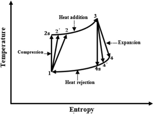
Figure 6. Simple cycle gas turbine.

2.4 Axial compressor model

Because the compressor performance dominates the total performance of GTs, it is generally advisable to base modeling GT performance largely on compressor features. The compressor performance beyond the design settings has been approximated using certain streamlining techniques. Some crucial performance data, however, such as the impact of varied stator blades or the surge margin, would be lost if the compressor shape is not known. Therefore, streamlining techniques should not be the first approach. The air properties at the compressor outlet ($\left.P_2,T_2,h_2,etc\right)$ must be calculated from the known characteristics at the intake ($\left.P_1,T_1,h_1,etc\right)$. First, it is necessary to change the map following the compressor IGVs and provide the setpoint of the compressor. The compressor variable ($m^{•},\mathit{PR},\eta$) is found in the map. Assuming an isentropic compression process ($S_1-S_2=0$), then $T_{2s}=T_1*{\left(\frac{p_2}{p_1}\right)}^{\frac{k-1}{k}}$.

The compressor inlet and discharge entropy $\left({\mathrm{s}}_1\&{\mathrm{s}}_2\right)$ can be calculated by using compressor inlet and isentropic discharge temperature $\left({\mathrm{T}}_1\&{\mathrm{T}}_{2\mathrm{s}}\right)$ in Eq. 17, and then, $T_2^{\prime }=T_{2s}*e^{-\left(\frac{{\mathit{s}}_{\mathbf{2}-}{\mathit{s}}_{\mathbf{1}}}{R}\right)}$. The compressor inlet and discharge enthalpy $\left({\mathrm{h}}_1\&h_2^{\prime }\right)$ can be calculated using the compressor inlet and isentropic discharge temperatures $\left({\mathrm{T}}_1\&T_2^{\prime }\right)$, and then, $h_2=h_1+\frac{\left(h_2^{\prime }-h_1\right)}{{ɳ}_c}$. The actual compressor discharge temperature (${\mathrm{T}}_2$) can be calculated using the bisection method.

2.5 Combustion system model

The real compressor airflow temperature (T₂) and combustion temperature (T₃) may be determined using the bisection approach. The combustor’s task is to ignite fuel using compressed gas released from the compressor with a minimal pressure drop. It is expected that the flow through the combustor will be continuous, 1D, and that no work will be done by the gases. The combustion process and the accompanying relationship may be established using the energy balance.

${\mathrm{M}}_{\mathrm{a}}^{•}\ast h_2+{ɳ}_b\ast {\mathrm{m}}_{\mathrm{f}}^{•}\ast \text{HV}=\left({\mathrm{m}}_{\mathrm{a}}^{•}+{\mathrm{m}}_{\mathrm{f}}^{•}\right)\ast h_3(18)$

The pressure drop via the combustor is thought to be related to the square of the flow rate variable approaching the combustor in the current study. It is thought to be 4% of the overall pressure at the combustor intake in the design load.

2.6 Axial turbine model

The turbine captures energy from the gas stream as it flows. Through this operation, the temperature and overall pressure both decrease, and the flow is adiabatic because heat transfer over the turbine is disregarded. From the known values at the turbine intake ($\left.P_3,T_3,h_3,etc\right)$, it is necessary to estimate the air properties at the turbine outlet ($\left.P_4,T_4,h_4,etc\right)$. The expansion process is thought to be isentropic ($S_4-S_3=0$), and then, $T_{4s}=T_3*{\left(\frac{p_4}{p_3}\right)}^{\frac{k-1}{k}}$. By using turbine inlet and isentropic exit temperature $\left({\mathrm{T}}_3\&{\mathrm{T}}_{4\mathrm{s}}\right)$ the turbine inlet and discharge entropy $\left({\mathrm{s}}_4\&{\mathrm{s}}_3\right)$ can be calculated, then $T_4^{\prime }=T_{4s}*e^{-\left(\frac{{\mathit{s}}_{\mathbf{3}-}{\mathit{s}}_{\mathbf{4}}}{R}\right)}$. The turbine inlet and discharge enthalpy $\left({\mathrm{h}}_3\&h_4^{\prime }\right)$ can be calculated by using turbine inlet and isentropic exit temperature $\left({\mathrm{T}}_3\&T_4^{\prime }\right)$, then $h_4=h_3-\frac{\left(h_3-h_4^{\prime }\right)}{{ɳ}_t}$. The turbine efficiency value was determined by using the actual discharge enthalpy and fuel/air ratio, and the actual discharge temperature was calculated inversely by using the bisection method. Then, the actual discharge temperature is used to calculate the actual discharge entropy.

2.7 Mathematic model operation system

The GT control system ensures that it operates safely and effectively. The GT is unable to run on its own at zero velocity. As a starting point, the shaft line’s self-sustaining speed is increased. The compressor bleed valves are up, and the IGVs are in the locked and shutdown state when the starting mechanism is activated. The cranking motor accelerates the GT to firing speed while the cranking torque from the initiating state disengages the turbine shaft. Fuel is fed into the combustion chamber. Two combustion chambers are ignited by spark plugs, and the flame travels to the remaining combustion chambers via the crossfire pipes. The starting motor is shut off by a GT speed threshold.

The bleed valve closes as the GT approaches optimum speed and transitions to full speed no load (FSNL) operation. The GT operates at the selected load (or part load) and base load after the circuit breaker is closed (full load). When “Preselected load” is chosen, the device will autonomously load or unload until the preselected load output is reached at the automatic loading rate. The megawatt setting for the preselected load is site-adjustable by altering the control constant. Fuel flow will be limited once the predetermined load level is reached in order to preserve that megawatt output.

When “base load” is chosen, the appliance will load normally up until the exit temperature control kicks in; at about this time, the appliance is operating at its nominal rated energy output for the surrounding environment. Fuel flow is controlled when the exit temperature control is engaged in order to give the machine the most power possible while avoiding “overfiring” it. It is significant to consider that the unit’s energy output will alter as environmental circumstances, particularly the temperature at the compressor input, fluctuate.

The airflow via the compressor, which controls the airflow throughout the entire system, is managed by the IGVs. The IGVs modulate during generator loading and unloading, GT startup and acceleration to rated speed, and shutdown. From zero to a maximum 85% of rated speed, the IGVs are kept fully shut at a nominal 34° at startup.

The IGVs will gradually open at approximately 6.7° for every percent increase in corrected speed after reaching a speed of approximately 85%. The IGVs will cease opening when they hit the lowest full-speed angle, which is typically 57°; this takes place at a speed lower than 100%. The IGVs will regulate to the fully open state when the output temperature is achieved as the unit is loaded and the exhaust temperature increases.

The IGVs should start to open when the exhaust temperature is within 17°C of the temperature control reference. As exhaust temperature reaches the temperature control remark, the IGVs move to the fully open position. The variable inlet guide vane schedule is depicted in Figure 7.

Figure 7

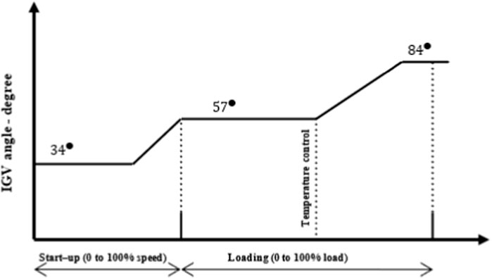
Figure 7. Variable inlet guide vane schedule.

2.8 Steady start and loading model

This section focuses on identifying the engine’s steady-state operating points from an idle speed of 60% to a design speed of 100% without loading and with loading at the design speed of 100%. It is necessary to describe the engine’s design position, its component features, and the operating fluid qualities as a function of temperature and the fuel-to-air ratio. The compressor pressure ratio and fuel flow rate are the two factors that are expected to be used as a reference factor to determine the optimal operating point on the compressor and turbine maps for each engine speed. Therefore, the following matching conditions must be met: mass continuity between the turbine and the compressor, $m_t=m_c+m_f$, power balance between compressor and turbine, $P_t=P_c$, and rotational speed, $N_t=N_c$.

The following steps summarize the matching procedure:

1. Define the IGV angle and modify the compressor map.

2. Select N/√T1. Suppose that the compressor’s working point is halfway between the first and final points in the sequence of chosen speed locations: $C_{o.p}=\left(\frac{C_{l.p}+C_{h.p}}{2}\right)$. Because the series has 14 points, $C_{h.p}=14,C_{l.p}=1$ for the first iteration.

3. Use interpolation to obtain the compressor operating point (${\pi }_c,m_c^{•},{ɳ}_c$) from the compressor map table.

4. Calculate he compressor discharge air properties ($T_2,P_2,h_2\&S_2$) from the axial compressor operating point (${\pi }_c,m_c^{•},{ɳ}_c$).

5. Assume the turbine inlet maximum temperature $T_{3\mathit{max}}=1200c^{⁰}$, turbine inlet minimum temperature $T_{3\mathit{min}}=T_2$, and the turbine inlet temperature $T_{3a}=\left(\frac{T_{3\mathit{max}}+T_{3\mathit{min}}}{2}\right)$ for the first iteration.

6. Calculate $\frac{\mathrm{N}}{\sqrt{\mathrm{T}3}\mathrm{a}}$ and $m_g^{•}=m_a^{•}+m_f^{•}$ so $m_f^{•}=\left(\frac{{\mathrm{m}}_{\mathrm{a}}^{•}\left({\mathrm{h}}_{3\mathrm{a}}-{\mathrm{h}}_2\right)}{\mathrm{H}.\mathrm{V}*{\mathrm{ɳ}}_{\mathrm{b}}-{\mathrm{h}}_{3\mathrm{a}}}\right)$ and use it to obtain the turbine operating point (${\pi }_t,{ɳ}_t$) from the turbine map table.

7. Calculate he turbine exits air properties ($T_4,P_4,h_4\&S_2$) from the axial turbine operating point (${\pi }_t,{ɳ}_t$).

8. Apply power balance $m_g^{•}\left(h_{3b}{-h}_4\right)=m_a^{•}\left(h_2{-h}_1\right)$ to obtain $h_{3b}$ and obtain $T_{3b}$ from $h_{3b}$.

9. If $\lceil T_{3a}-T_{3b}\rceil \prec 0$, obtain $T_{3\mathit{min}}$ =$T_{3a}$ and repeat Step 5 through Step 8.

10. If $\lceil T_{3a}-T_{3b}\rceil \succ 0$, obtain $T_{3\mathit{max}}$ = $T_{3a}$ and repeat Step 5 through Step 8.

11. If $\lceil T_{3a}-T_{3b}\rceil \approx 0$, the turbine inlet temperature is correct.

12. Calculate ${∆p}_{err}={∆p}_c-{∆p}_b-{∆p}_t$, where ${∆p}_c$: compressor differential pressure, ${∆p}_b$: combustion chamber differential pressure, and ${∆p}_t$: turbine differential pressure.

13. If $\lceil {∆p}_{err}\rceil \prec 0$, obtain $C_{l.p}=C_{o.p}$ and repeat Step 2 through Step 12.

14. If $\lceil {∆p}_{err}\rceil \succ 0$, obtain $C_{h.p}=C_{o.p}$ and repeat Step 2 through Step 12.

15. If $\lceil {∆p}_{err}\rceil \approx 0$, the matching is complete.

3 Results and discussion

This section reports the results of the steady start model, the effect of the IGV system for steady start performance, a comparison between the steady start model and field data, the loading model, the effect of the IGV system for the loading model, and a comparison between the loading model with field data. In this study, a mathematical model constructed using the MATLAB program was used to calculate steady-state performance for a single spool industrial gas turbine engine during both startup (64%–100% design speed) and loading (100% design speed). The variations of the working fluid thermodynamic properties with both temperature and fuel-to-air ratio are considered. An iterative method was used by assuming the operating points for both the turbine and compressor. If the assumption is correct, matching constraints (continuity and power balance) must be satisfied. Otherwise, some errors representing the component mismatching will arise. The results obtained for the investigated parameters are discussed in the following sections.

3.1 Steady start model results

The variations in compressor pressure ratio, fuel and exhaust gas mass flow rate, and operating temperatures against engine startup speed ratio are shown in Figure 8. It can be seen from the figure that all the variables increase when the engine startup speed ratio increases, except the turbine outlet temperature, which decreases as the engine startup speed ratio increases. In addition, the figure shows that in the steady start model, the compressor pressure ratio, fuel and exhaust gas mass flow rate, compressor outlet temperature, and turbine inlet temperature increased by 140%, 100%, 132%, 32%, and 9%, respectively, while the turbine outlet temperature decreases by 7% when the engine startup speed ratio increases from 0.63 to 1.

Figure 8

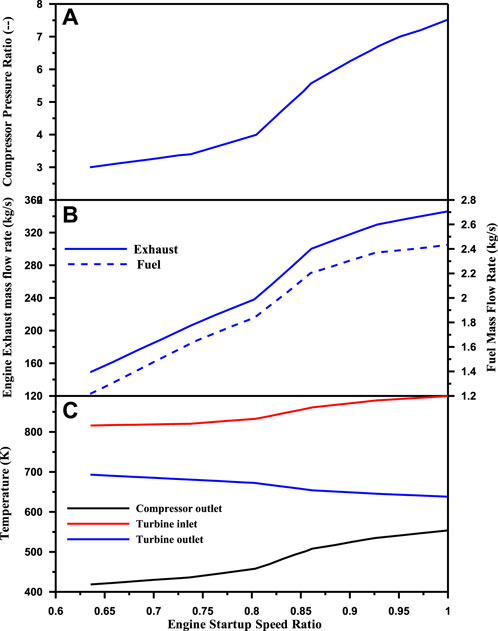
Figure 8. Variation of (A) compressor pressure ratio, (B) fuel and exhaust gas mass flow rate, and (C) operating temperatures against the engine startup speed ratio.

3.2 Effect of the IGV system on steady start performance

Figure 9 shows the effect of the IGVs on operating temperatures against the engine startup speed ratio. When the engine startup speed ratio increases, the compressor outlet temperature and turbine inlet temperature increase, while the turbine outlet temperature decreases with and without the IGVs. In addition, it is evident from the figure that the average compressor outlet temperature and average turbine inlet temperature decreased by 11.2% and 1.2% when using the IGVs, while the average outlet temperature increased by 10%.

Figure 9

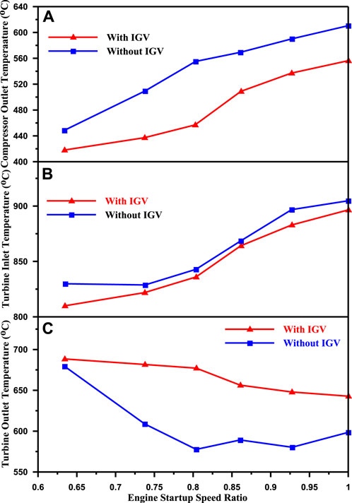
Figure 9. Effect of IGVs on operating temperatures against the engine startup speed ratio. (A) Compressor pressure ratio, (B) Fuel and exhaust gas mass flow rate and (C) Operating temperatures.

Figure 10 shows the effect of engine startup speed ratio on compressor pressure ratio, fuel and exhaust gas mass flow rate, and compressor-driven power with and without IGVs. It is evident from the figure that, by using the IGVs, the average compressor pressure ratio, fuel and exhaust gas mass flow rate, and compressor-driven power decreased by 33.4%, 9.5%, 19.3%, and 37.5%, respectively.

Figure 10

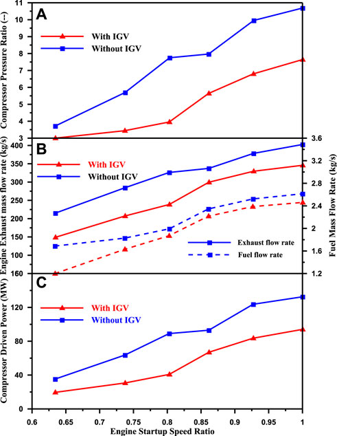
Figure 10. Effect of engine startup speed ratio on (A) compressor pressure ratio, (B) fuel and exhaust gas mass flow rate, and (C) compressor-driven power, with and without IGVs.

3.3 Comparing steady start results with field data

The steady start model results are compared with field data from a 9EA-GT that give all the variables against engine relative speed in Figures 11, 12. It is clear from the figures that the simulation results are in good agreement with the real engine data. Average errors of 1%, 0.8%, 2.2%, 4%, 2.7%, and 6.9% were found for compressor outlet temperature, turbine inlet temperature, turbine outlet temperature, compressor compression ratio, exhaust mass flow rate, and fuel mass flow rate, respectively.

Figure 11

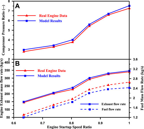
Figure 11. Compression between real engine data and model performance parameter results against the engine startup speed ratio. (A) Compressor pressure ratio, (B) Fuel and exhaust gas mass flow rate.

Figure 12

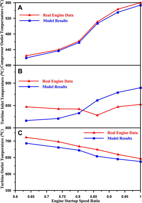
Figure 12. Compression between real engine data and model operating temperature results against the engine startup speed ratio. (A) Compressor pressure ratio, (B) Fuel and exhaust gas mass flow rate and (C) operating temperatures.

3.4 Loading model result

The variations in compressor pressure ratio, fuel and exhaust gas mass flow rate, and operating temperatures against engine output power are shown in Figure 13. It can be seen from the figure that all the variables increase when engine output power increases. In addition, it is evident from the figure that the compressor pressure ratio, fuel and exhaust gas mass flow rate, compressor outlet temperature, turbine inlet temperature, and turbine outlet temperature increased by 46%, 14%, 150%, 32.2%, 47.9%, and 27.9%, respectively.

Figure 13

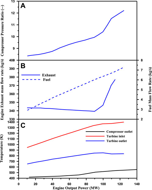
Figure 13. Variation of (A) compressor pressure ratio, (B) fuel and exhaust gas mass flow rate, and (C) operating temperatures against engine output power.

3.5 Effect of the IGV system on loading performance

Figure 14 shows the effect of IGVs on operating temperatures against engine output power. When engine output power increases, the compressor outlet temperature, turbine inlet temperature, and turbine outlet temperature increase with and without IGVs. In addition, it is evident from the figure that the average turbine inlet temperature and the average outlet temperature increase by 3.8% and 8.1%, respectively. Meanwhile, the average compressor outlet temperature decreases by 4.6%.

Figure 14

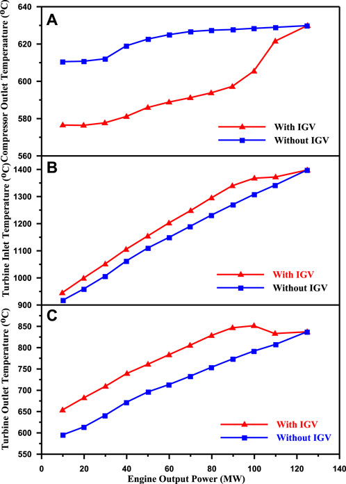
Figure 14. Effect of IGVs on operating temperatures against engine output power. (A) Compressor pressure ratio, (B) Fuel and exhaust gas mass flow rate and (C) operating temperatures.

Figure 15 shows the variation of compressor pressure ratio, fuel and exhaust gas mass flow rate, and compressor-driven power against the engine output power with and without IGVs. It is evident from the figure that by using the IGVs, the average compressor pressure ratio, fuel mass flow rate, exhaust gas mass flow rate, and compressor-driven power decreased by 16.9%, 1%, 12.2%, and 19.7%, respectively.

Figure 15

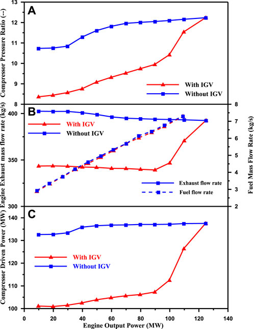
Figure 15. Effect of engine output power on (A) compressor pressure ratio, (B) fuel and exhaust gas mass flow rate, and (C) compressor-driven power, with and without IGVs.

3.6 Comparing loading results with field data

Loading model results are compared with field data from a 9EA-GT against engine relative speed in Figures 16, 17. It is clear from the figures that the simulation results have good agreement with the real engine data and have average errors of 0.6%, 1.6%, 5.8%, 2%, 1.6%, and 3.1% for compressor outlet temperature, turbine inlet temperature, turbine outlet temperature, compressor compression ratio, exhaust mass flow rate, and fuel mass flow rate, respectively.

Figure 16

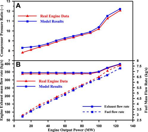
Figure 16. Compression between real engine data and model result performance parameters against the engine startup speed ratio. (A) Compressor pressure ratio, (B) Fuel and exhaust gas mass flow rate.

Figure 17

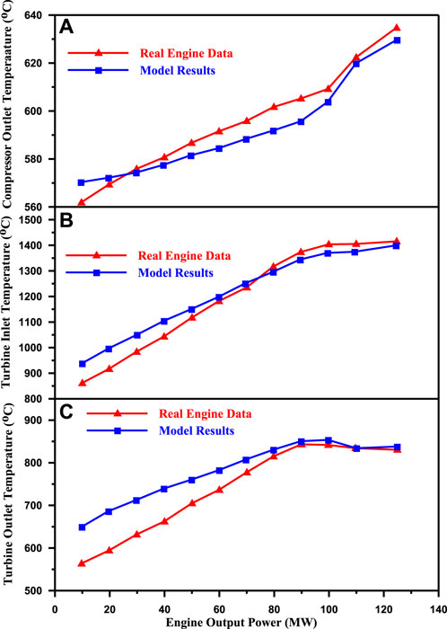
Figure 17. Compression between real engine data and model operating temperature results against the engine startup speed ratio. (A) Compressor pressure ratio, (B) Fuel and exhaust gas mass flow rate and (C) operating temperatures.

4 Conclusion

This article presents a model-based performance study for the single spool 9EA-GT developed by General Electric. A novel component map production method that can recognize component features was developed for this model using the system detection approach to develop the component maps that have a significant impact on performance simulation in contrast to the minimal map supplied by the engine manufacturer. The control of engine flow capacitance by changing the IGVs of the first stages of the axial compressor was studied, and this led to a change in the axial compressor map. MATLAB was used to simulate engine performance using the obtained component maps to achieve steady-state performance assessment under different working conditions. Assessment results utilizing the suggested model agreed with the actual performance data with a manageable margin of error and validated the suggested engine performance model.

Two models were used in the calculations for steady-state performance: one for the engine’s steady-state behavior during startup (from 65% to 100% speed, without load) and another for the engine’s steady-state behavior under loading (constant speed). The difficulties caused by the lack of knowledge of stage-by-stage performance have been addressed in this model by creating artificial machine maps, validating them with experimental observations from actual power plants, and applying appropriate scaling techniques to generalized maps derived from earlier research. The current study is concerned with studying flow angles without taking the deviation from the flow angles at various operating modes of the gas turbine into account. The deviation from the flow angles at various operating modes of the gas turbine could be studied in future work.

The efficiencies of GTE components are affected by changes in the operating conditions. In this study, with changes in operating conditions, the compressor efficiency changed from a maximum of 81.4% to a minimum of 76.5%, the turbine efficiency changed from a maximum of 82.1% to a minimum of 78.8%, and the combustion efficiency for the combustion chamber changed from a maximum of 81.4% to a minimum of 76.5%.

Data availability statement

The original contributions presented in the study are included in the article/Supplementary Material; further inquiries can be directed to the corresponding author.

Author contributions

AA: conceptualization, methodology, validation, visualization, writing–original draft, and writing–review and editing.

Funding

The author(s) declare that no financial support was received for the research, authorship, and/or publication of this article.

Acknowledgments

The author would like to thank the Deanship of Scientific Research at Shaqra University for supporting this work.

Conflict of interest

The author declares that the research was conducted in the absence of any commercial or financial relationships that could be construed as a potential conflict of interest.

Publisher’s note

All claims expressed in this article are solely those of the authors and do not necessarily represent those of their affiliated organizations, or those of the publisher, the editors, and the reviewers. Any product that may be evaluated in this article, or claim that may be made by its manufacturer, is not guaranteed or endorsed by the publisher.

References

Asgari, H., Chen, X., Menhaj, M. B., and Sainudiin, R. (2013). Artificial neural network based system identification for a single-shaft gas turbine. J. Eng. Gas Turbines Power 135 (9). doi:10.1115/1.4024735

CrossRef Full Text | Google Scholar

Awang Saifudin, A. R., and Mazlan, N. M. (2014). Computational exploration of a two-spool high bypass turbofan engine's component deterioration effects on engine performance. Appl. Mech. Mater. 629, 104–108. doi:10.4028/www.scientific.net/amm.629.104

CrossRef Full Text | Google Scholar

Cohen, H., Rogers, C. F. C., and Saravanamuttoo, H. I. H. (1987). Gas turbine theory. 3rd edition. Essex, Great Britain: Longman Scientific and Technical, Longman Group Limited.

Google Scholar

Farahat, M. A., and Talaat, M. (2012). The using of curve fitting prediction optimized by genetic algorithms for short-term load forecasting. Int. Rev. Electr. Eng. (IREE) 7 (6), 6209–6215.

Google Scholar

Li, J., Ouazzane, K., Kazemian, H., Jing, Y., and Boyd, R. (2011). A neural network based solution for automatic typing errors correction. Neural Comput. Appl. 20 (6), 889–896. doi:10.1007/s00521-010-0492-3

CrossRef Full Text | Google Scholar

Liu, Q., and Cao, J. (2010). A recurrent neural network based on projection operator for extended general variational inequalities. IEEE Trans. Syst. Man, Cybern. Part B 40 (3), 928–938. doi:10.1109/tsmcb.2009.2033565

PubMed Abstract | CrossRef Full Text | Google Scholar

Liu, Q., Cao, J., and Chen, G. (2010b). A novel recurrent neural network with finite-time convergence for linear programming. Neural Comput. 22, 2962–2978. doi:10.1162/neco_a_00029

PubMed Abstract | CrossRef Full Text | Google Scholar

Liu, Q., Dang, C., and Cao, J. (2010a). A novel recurrent neural network with one neuron and finite-time convergence for k-winners-take-all operation. IEEE Trans. Neural 21 (7), 1140–1148. doi:10.1109/TNN.2010.2050781

PubMed Abstract | CrossRef Full Text | Google Scholar

McBride, B. J., Zehe, M. J., and Gordon, S., "NASA glenn coefficients for calculating thermodynamic properties of individual species", https://ntrs.nasa.gov/citations/20020085330, 2002.

Google Scholar

Meng, W., Song, D., Huang, L., Chen, X., Yang, J., Dong, M., et al. (2023). Robust pricing strategy with EV retailers considering the uncertainty of EVs and electricity market. Beijing, China: Tsinghua-IET Electrical Engineering Academic Forum 2023, 27–33. doi:10.1049/icp.2023.1827

CrossRef Full Text | Google Scholar

Meng, W., Song, D., Huang, L., Chen, X., Yang, J., Dong, Mi, et al. (2024a). A Bi-level optimization strategy for electric vehicle retailers based on robust pricing and hybrid demand response. Energy 289, 129913. doi:10.1016/j.energy.2023.129913

CrossRef Full Text | Google Scholar

Meng, W., Song, D., Huang, L., Chen, X., Yang, J., Dong, Mi, et al. (2024b). Distributed energy management of electric vehicle charging stations based on hierarchical pricing mechanism and aggregate feasible regions. Energy 291, 130332. doi:10.1016/j.energy.2024.130332

CrossRef Full Text | Google Scholar

Morini, M., Pinelli, M., Spina, P. R., and Venturini, M. (2010). Computational fluid dynamics simulation of fouling on axial compressor stages. J. Eng. Gas Turbines Power 132 (7). doi:10.1115/1.4000128

CrossRef Full Text | Google Scholar

Najmi, W. M. W. A., and Arhosazani, A. M. (2006). “Comparison of combustion performance between natural gas and medium fuel oil at different firing settings for industrial boilers,” in Conference: International Conference on Energy and Environment (ICEE), Portugal, 7th June 2006.

Google Scholar

Nikpey, H., Assadi, M., and Breuhaus, P. (2013). Development of an optimized artificial neural network model for combined heat and power micro gas turbines. Appl. Energy 108, 137–148. doi:10.1016/j.apenergy.2013.03.016

CrossRef Full Text | Google Scholar

Ogaji, S. O. T., Sampath, S., Marinai, L., Singh, R., and Probert, S. D. (2005). Evolution strategy for gas-turbine fault-diagnoses. Appl. Energy 81, 222–230. doi:10.1016/j.apenergy.2004.07.003

CrossRef Full Text | Google Scholar

Ogbonnaya, E. A. (2011). Gas turbine performance optimization using compressor online water washing technique. Engineering 3 (5), 500–507. doi:10.4236/eng.2011.35058

CrossRef Full Text | Google Scholar

Palmé, T., Fast, M., and Marcus, Thern (2011). Gas turbine sensor validation through classification with artificial neural networks. Appl. Energy 88, 3898–3904. doi:10.1016/j.apenergy.2011.03.047

CrossRef Full Text | Google Scholar

Razak, A. M. Y. (2007). Industrial gas turbines performance and operability. CB21 6AH, England, UK: CRC Press: Published by Woodhead Publishing Limited Cambridge.

Google Scholar

Roumeliotis, I. (2010). Degradation effects on marine gas turbines. Piraeus, Greece: Hellenic Naval Academy.

Google Scholar

SadoughVanini, Z. N., Khorasani, K., and Meskin, N. (2014). Fault detection and isolation of a dual spool gas turbine engine using dynamic neural networks and multiple model approach. Inf. Sci. 259, 234–251. doi:10.1016/j.ins.2013.05.032

CrossRef Full Text | Google Scholar

Song, D., Tan, X., Deng, X., Yang, J., Dong, Mi, Elkholy, M. H., et al. (2023). Rotor equivalent wind speed prediction based on mechanism analysis and residual correction using Lidar measurements. Energy Convers. Manag. 292, 117385. doi:10.1016/j.enconman.2023.117385

CrossRef Full Text | Google Scholar

Talaat, M., Alblawi, A., Tayseer, M., and Elkholy, M. H. (2022). FPGA control system technology for integrating the PV/wave/FC hybrid system using ANN optimized by MFO techniques. Sustain. Cities Soc. 80, 103825. doi:10.1016/j.scs.2022.103825

CrossRef Full Text | Google Scholar

Talaat, M., Elgarhy, A., Elkholy, M. H., and Farahat, M. A. (2021). Integration of fuel cells into an off-grid hybrid system using wave and solar energy. Int. J. Electr. Power & Energy Syst. 130, 106939. doi:10.1016/j.ijepes.2021.106939

CrossRef Full Text | Google Scholar

Talaat, M., Elkholy, M. H., Alblawi, A., and Said, T. (2023). Artificial intelligence applications for microgrids integration and management of hybrid renewable energy sources. Artif. Intell. Rev. 56, 10557–10611. doi:10.1007/s10462-023-10410-w

CrossRef Full Text | Google Scholar

Talaat, M., Farahat, M. A., and Elkholy, M. H. (2019). Renewable power integration: experimental and simulation study to investigate the ability of integrating wave, solar and wind energies. Energy 170, 668–682. doi:10.1016/j.energy.2018.12.171

CrossRef Full Text | Google Scholar

Talaat, M., Gobran, M. H., and Wasfi, M. (2018). A hybrid model of an artificial neural network with thermodynamic model for system diagnosis of electrical power plant gas turbine. Eng. Appl. Artif. Intell. 68, 222–235. doi:10.1016/j.engappai.2017.10.014

CrossRef Full Text | Google Scholar

Tayseer, M., Talaat, M., and Farahat, M. A. (2024). Optimum design of spacer material of gas-insulated switchgear by utilizing the technology of functionally graded material using different artificial optimization techniques. Surf. Coatings Technol. 479, 130530. doi:10.1016/j.surfcoat.2024.130530

CrossRef Full Text | Google Scholar

Walsh, P. P., and Fletcher, P. (1998). Gas turbine performance. Blackwell Science Ltd.

Google Scholar

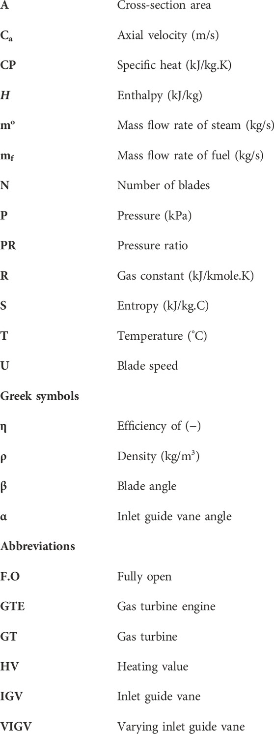
Nomenclature