Sensitivity analysis for the EEG forward problem

Introduction

The electric process underlying the generation of the electroencephalography (EEG) signals can be modeled as a set of current sources within the brain. Considering the velocity of propagation of the electric waves in the brain, the static approximation of Maxwell’s equations can be used to describe this process (see Hamalainen et al., 1993). The resulting model is a 3D Poisson-type equation with interfaces that relates the electric potential u in the head G with the impressed current J_i often represented by an electric dipole, i.e., J_i(x) = Mδ(x − q), where δ is the Dirac distribution, q is a fixed point in the brain which represents the dipole location, and M is the dipole moment. The parameters of the model are the conductivity of the different tissues, σ(x), x ∈ G, the diameters of the different compartments of the head, and the moment and location of the dipole: M ∈ R³, q ∈ G respectively. The forward problem (FP) of EEG consists in finding the electric potential u in the head for a given current source J_i. Conversely the inverse problem (IP) of EEG consists in finding the location q that produces a given scalp data u. An accurate solution to the IP could provide useful information to treat neurological diseases such as epilepsy. In order to solve the IP we need first to solve the FP. In this context it is important to analyze the sensitivity of the solutions to the FP with respect to the different parameters of the model since this information could help us to choose the points on the scalp where the data are to be collected.

In the literature two different sensitivity functions are frequently used: the traditional sensitivity functions (TSF) defined as ∂u/∂θ that measures the variations of the output u when the parameter θ changes and the generalized sensitivity functions (GSF) that determine at which time instants the output of a dynamical system has more information about the value of its parameters in order to carry on an estimation process.

In this work we consider the head as a multi compartment nested set and assume homogeneity and isotropy, hence the conductivity function σ(x) that contains the value of the conductivity of the different tissues is approximated by a positive piecewise constant function. We analyze the sensitivity of the solution u to the FP with respect to the conductivity σ(x) by means of the TSF and the GSF and compare the results.

The paper is organized as follows. In Section “The Mathematical Model” we present the mathematical model. The TSF are introduced in Section “Materials and Methods.” Differential and integral equations are stated. In Section “Results,” we present the GSF. Based on Rubio et al. (2009) we calculate the GSF of u with respect to σ(x). We performed numerical experiments in a simple head model and present some conclusions.

The Mathematical Model

The electrical activity of the brain consists of currents generated by biochemical sources at cellular level. The electric and magnetic fields that they produce can be estimated by means of Maxwell’s equations (see Sarvas, 1987; Hamalainen et al., 1993). Based on the properties of the tissues involved, the velocity of propagation of the electromagnetic waves caused by potential changes within the brain is such that the effect may be detected simultaneously at any point in the brain or in the surrounding tissues. This fact justifies the use of a static approximation of Maxwell’s equations. This approximation uncouples the equations for the magnetic and electric fields leading to the following second order partial differential equation (PDE)

that relates the measured electric potential u and the impressed current J_i.

The volume G (head model) consists of nested homogeneous sets, one surrounded by the next one where the conductivity values are given.

We consider , denoted from the inner one to the outer one by: G₁, the brain, G₂, the skull, and G₃, the scalp. We denote Γ = ∂G the external surface of G and by S₁ = ∂G₁, S₂ = ∂G₂ − ∂G₁ the surfaces between G₁ and G₂ and G₂ and G₃ respectively.

The positive, discontinuous and piecewise constant function σ(x) that contains the conductivity values of the different tissues at each point is:

Assuming that the potential and its normal derivative times the conductivity function are continuous across the transition surfaces, the resulting boundary value problem is:

subject to:

where [·] denotes the difference between the values of the functions inside the brackets through the indicated surface, ν is the external normal vector and F(x) = ▽·J_i(x).

If F is regular enough, there exist solutions (in a weak sense) to (3) provided that F verifies They are unique up to a constant (see Troparevsky and Rubio, 2003).

When J_i is an electric dipole, existence and uniqueness of solutions were studied in El Badia (2000).

Materials and Methods

Traditional Sensitivity Functions

The TSF is a common tool used to measure the variation of the output u of a system with respect to changes in its parameter θ = (θ₁, θ₂,…,θ_p). Assuming smoothness of u, they are defined as the partial derivative of u with respect to each θ_i, namely:

The sensitivity functions are related to u by the Taylor approximation of first order. In the case of the system modeled by equations (1)–(5), considering u as a function of x ∈ G and the vector of parameters θ = (σ₁, σ_3, σ₃), i.e., u = u(x, σ₁, σ₁, σ_3, σ₃) and fixing x, σ₂, σ₃, we have:

u(x, σ₁ + Δ, σ_2, σ₃) ≅ u(x, σ₁, σ₂, σ₃) + s₁(x, σ₁, σ₂, σ₃)Δ

These functions s_i(x) give local information and are used to determine the parameter to which the model is more sensitive. Note that the value of s_i(x) depends on the dimensions and the units of the parameter θ_i, then, in order to compare the sensitivity with respect to different parameters “normalized sensitivities” can be introduced, where the quotient between the relative errors of the output (numerator) and the relative error of the parameter (denominator) is considered.

In the next subsection we derive the differential sensitivity equations (see Stanley, 1999; Burns et al., 2005) for the interface problem (3)–(5) introduced in Section “The Mathematical Model.”

Differential equations for the TSF

We consider three parameters in our model: the conductivity values for each sub domain G_i, i.e., σ₁, σ₂, σ_3. Thus the vector of parameters is θ = (θ₁, θ_2, θ₃) = (σ₁, σ₂, σ₃), and the sensitivity functions to be considered are:

These functions satisfy the following state equations that can be derived from (3) by formal differentiation (see Stanley, 1999):

The boundary condition for each s_i can be derived from (4) observing that the normal ν on the external surface Γ = ∂G does not depend on the σ_i, i = 1, 2, 3.

The equations (5) of continuity of u at the transition surfaces lead to:

and,

Note that in order to solve the PDE systems that correspond to the sensitivity functions s_i(x) one needs the values of u and ∂u/∂v on the transition surfaces and the value of the Laplacian Δu on G.

As for the equation (3), the sensitivity equations may only have solution in a weak sense.

Integral equations

Integral equations for the sensitivity functions can also be stated. They are useful to perform numerical approximations. We present the ones corresponding to s₁(x).

Recall that s₁ satisfies:

with boundary condition:

and interface conditions:

Applying green integral identity:

in each G_i, i = 1,2 and choosing Φ such that ΔΦ(x, y) = −4πδ(x − y), i.e., Φ(x, y) = 1/|x − y| we arrive to:

Combining the former equation with (7), the boundary condition (9) and the continuity conditions at the transition surfaces (10) we obtain:

If we take x ∈ G₁ in (13), since σ₁Δu = F in G₁ we obtain:

Similarly we can choose x ∈ G₂ or x ∈ G₃ to obtain the corresponding integral equations.

Remark Note that only the values of s₁ on the transition surfaces appear in the right hand side of (14).

Letting in (14), and recalling that:

we can obtain an equation involving only values of s₁ on the transition surfaces.

Generalized Sensitivity Function

The GSF was introduced by Thomaseth and Cobelli (1999) to analyze qualitatively where the information about model parameters is concentrated during identification experiments. It was meant to understand how the estimation is related to observed system outputs, taking into account correlations between the model parameters. We recall the definition and some properties of the GSF, for details we refer to Thomaseth and Cobelli (1999).

Consider a non-linear parametric dynamical system:

with a set of discrete time observations at t₁…t_n:

where u(t), f(t, u, θ), ∈ R^N, θ ∈ R^p, h(t, θ) ∈ R, and e_j, ∈ R is the measurement noise assumed to be independently and identically distributed with zero mean and known variance . It is assumed that there exists a true θ₀ such that the observed data y_j correspond to that parameter value.

Let us consider the minimization of the weighted residual sum of squares:

A value where the minimum is attained is an estimator of θ₀.

The GSF at t_k are defined as:

where F is the corresponding p × p Fisher information matrix:

and the symbol “·” in (20) represents element-by-element vector multiplication and ▽_θh is the gradient that contains the derivatives of h with respect to each component of the parameter vector θ, that is the sensitivity of h with respect to the parameters. Thus, GSF are defined only at the discrete time points t₁,…,t_n where measurements are taken. Note that gs(t_k) involves all the contributions of those measurements up to and including t_k. On the other hand the incremental GSF (GSF_inc), defined by:

gives the information provided by the single measurements t_k. Note from (20) and (21) that the TSF have to be calculated in order to compute the GSF.

Remark The relationship between the GSF and the estimator of θ becomes clear if we introduce a continuous version of the parameter estimation problem supposing we have the measurements of the output for all t ∈ [0,T]. In this case the minimization of J in (19) can be thought in a space of probability (continuous version) leading to:

where t_j ∈ [0,T] and P is a probability function defined in [0,T]. In this frame the Fisher information matrix becomes and its inverse is, asymptotically and approximately, the covariant matrix of the estimator of θ. The generalized sensitivity at t ∈ [0,T] is the diagonal of (see Banks et al., 2008).

Now we can come back to the FP of EEG modeled by equations (1)–(5). In this case we cannot calculate the GSF corresponding to the PDE system that models the FP of EEG straightforward since instead of a dynamical system, in this case the independent variable is x ∈ G ⊂ R³. The available data is now the value of the potential u at given points on the scalp x_j contaminated with noise and the observations are given by:

where the observation errors e_j ∈ R are assumed to satisfy the standard statistical assumptions. We assume that there exists a value parameter θ₀ such that the data set {y_j} has the form given in (23) when θ = θ₀.

In Rubio et al. (2009) it was proved that choosing an arbitrary order for the observation points x_j, the function:

is well-defined, that is, the value of GSF_inc(x) at a given observation point x ∈ ∂G does not depend on the order given to the observations points. Thus, we choose an order for the observation points on the scalp and perform the calculations.

Results

We calculate the TSF and the GSF of u with respect to σ₁ for a dipole source J_i(x) = Mδ(x − q) for different locations q ∈ G₁ in a spherical head model. This approximation for the head allows us to calculate the solution by the series formula appearing in Zhang (1995). Differentiating this series with respect to σ₁ we obtain the sensitivity function s₁ for the case of nested homogeneous spherical sets. We compare their values to find out the information that they provide about the variations on the scalp potential u when σ₁ changes. The values of the sensitivities were simulated considering that the observations are measurements of the electric potential on the scalp collected by means of a set of electrodes with 10-10B configuration and that the “spike-instants” where the values of u are considered, were detected and marked on the data by experts. We consider the conductivity values in (2): σ₁ = 0.33, σ₂ = 0.0042, σ₃ = 0.33(1/(Ω/m)) (see Geddes and Baker, 1967). We choose an order to enumerate the electrode positions and calculate the GSF_inc and the TSF with respect to σ₁ for different radial and tangential dipoles. The results obtained are shown in the figures below. Since no comparison between sensitivities for different parameters is presented, we have not normalized the values and have plotted the values of the absolute value of TSF directly. In Figure 1 we plot the values of GSF_inc at the 20 electrode positions for the same dipole location r_q = (0.3, 0.4, 0) and different dipoles moments, a radial one M = (3, 4, 0) and a tangential one M = (−4, 3, 0).

FIGURE 1

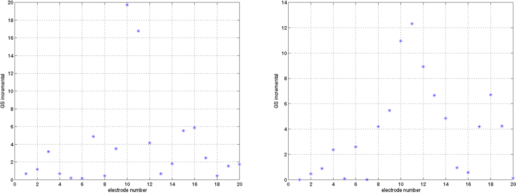
Figure 1. Generalized sensitivity GSF_inc (in absolute value) for the dipole position r_q = (0. 3, 0.4, 0) and different moments: Right: M = (3, 4, 0) (radial) Left: M = (−4, 3, 0).

In Figure 2, we show the absolute value of the TSF on the scalp for the same dipole location r_q = (0.3, 0.4, 0) and different dipoles moments. The stars indicate the positions of the scalp electrodes. In order to compare both sensitivity functions we have put an M at the position of the electrode where the two highest values of GSF_inc are achieved.

FIGURE 2

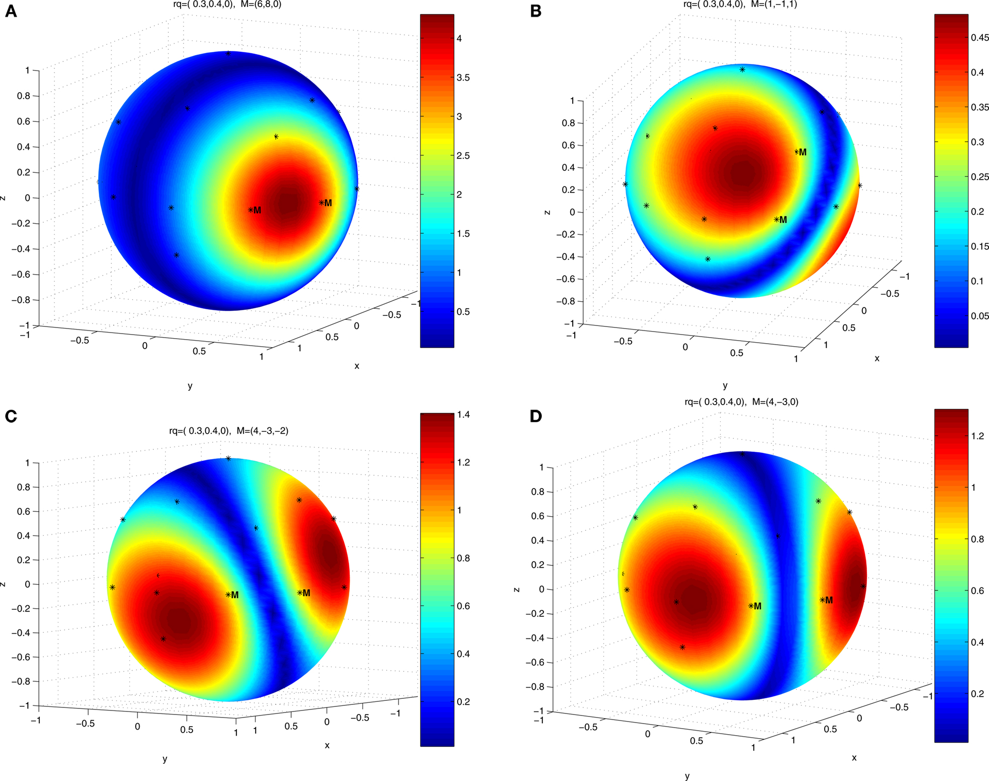
Figure 2. Traditional sensitivity functions (in absolute value) for the dipole position r_q = (0. 3, 0.4, 0) and different moments (DM) M, (A) DM M = (6, 8, 0) (radial) (B) DM M = (1, −1, 1) (C) DM M = (4, 3, −2) (D) DM M = (4, −3, 0) (tangential).

Discussion

From the experiments we conclude that in this example TSF and GSF do not seem to provide the same information. It can be noted that in Figures 2B and D the maximum is not located at the electrode where TSF would suggest. Since the GSF is defined taking into account the influence that parameter variations have on the estimator , theoretically it seems to be more suitable to look at the values of the GSF before performing the parameter estimation. More examples in different domains had to be performed and a theoretical analysis about the information provided of both sensitivity functions must be done. In future, based on these sensitivities, an optimal distribution of scalp electrodes may be determined in order to estimate the parameters of the model.

Conflict of Interest Statement

The authors declare that the research was conducted in the absence of any commercial or financial relationships that could be constructed as a potential conflict of interest.

Acknowledgements

This research was supported in part by the Air Force Office of Scientific Research under grant FA9550-10-1-0037

References

Banks, H. T., and Bihari, K. L. (2001). Modeling and estimating uncertainty in parameter estimation. Inverse Probl. 17, 95–111.

CrossRef Full Text

Banks, H. T., Dediu, S., and Ernstberger. S. L. (2008). Sensitivity functions and their uses in inverse problems. J. Inverse III-Posed Probl. 15, 683–708, ISSN (Online) 1569–3945.

Burns, J. A., Lin, T., and Stanley, L. (2005). A Petrov-Galerkin finite element method for interface problems arising in sensitivity computations. Comput. Math. Appl. 49, 1889–1903.

CrossRef Full Text

El Badia, A. (2000). Inverse source problem in an anisotropic medium by boundary measurements. Inverse Probl. 16, 651–663.

CrossRef Full Text

Geddes, L. A., and Baker, L. E. (1967). The specific resistant of biological materials – a compendium of data for the biomedical engineering and physiologist. Med. Biol. Eng. 5, 271–293.

Pubmed Abstract | Pubmed Full Text | CrossRef Full Text

Hamalainen, M., Hari, R., Ilmoniemi, R. J., Knuutila, J., and Lounasmaa, O. (1993). Magnetoencephalography, theory, instrumentation and applications to noninvasive studies of the working human brain. Rev. Mod. Phys. 65, 414–487.

CrossRef Full Text

Kappel, F., and Batzel, J. (2006). “Sensitivity analysis of a model of the cardiovascular system,” in Proceedings of the 28th IEEE EMBS Annual International Conference, New York.

Rubio, D., Troparevsky, M. I., and Saintier, N. (2009). “Generalized sensitivity analysis for an elliptic equation with interfaces,” in Proceedings of XIII Reunión de trabajo en procesamiento de la Información y control, RPIC 09, Rosario, Argentina.

Sarvas, J. (1987). Basic mathematical and electromagnetic concepts of the biomagnetic inverse problem. Phys. Med. Biol. 32, 11–22.

Pubmed Abstract | Pubmed Full Text | CrossRef Full Text

Stanley, L. G. (1999). Computational Methods for Sensitivity Analysis with Applications to Elliptic Boundary Value Problems. Ph.D. thesis, Department of Mathematics, Virginia Tech, Blacksburg, VA.

Thomaseth, K., and Cobelli, C. (1999). Generalized sensitivity functions in physiological system identification. Ann. Biomed. Eng. 27, 607–616.

Pubmed Abstract | Pubmed Full Text | CrossRef Full Text

Troparevsky, M. I., and Rubio, D. (2003). On the weak solutions of the forward problem in EEG. J. Appl. Math. 12, 647–656.

CrossRef Full Text

Zhang, Z. (1995). A fast method to compute surface potentials generated by dipoles within multilayer anisotropic spheres. Phys. Med. Biol. 40, 335–349.

Pubmed Abstract | Pubmed Full Text | CrossRef Full Text