The flatness of bifurcations in 3D dendritic trees: an optimal design
- 1 Computational Neuroscience Group, Department of Integrative Neurophysiology, Center for Neurogenomics and Cognitive Research, VU University Amsterdam, Amsterdam, Netherlands
- 2 Department of Anatomy and Neuroscience, VU University Medical Center, Amsterdam, Netherlands
The geometry of natural branching systems generally reflects functional optimization. A common property is that their bifurcations are planar and that daughter segments do not turn back in the direction of the parent segment. The present study investigates whether this also applies to bifurcations in 3D dendritic arborizations. This question was earlier addressed in a first study of flatness of 3D dendritic bifurcations by Uylings and Smit (1975), who used the apex angle of the right circular cone as flatness measure. The present study was inspired by recent renewed interest in this measure. Because we encountered ourselves shortcomings of this cone angle measure, the search for an optimal measure for flatness of 3D bifurcation was the second aim of our study. Therefore, a number of measures has been developed in order to quantify flatness and orientation properties of spatial bifurcations. All these measures have been expressed mathematically in terms of the three bifurcation angles between the three pairs of segments in the bifurcation. The flatness measures have been applied and evaluated to bifurcations in rat cortical pyramidal cell basal and apical dendritic trees, and to random spatial bifurcations. Dendritic and random bifurcations show significant different flatness measure distributions, supporting the conclusion that dendritic bifurcations are significantly more flat than random bifurcations. Basal dendritic bifurcations also show the property that their parent segments are generally aligned oppositely to the bisector of the angle between their daughter segments, resulting in “symmetrical” configurations. Such geometries may arise when during neuronal development the segments at a newly formed bifurcation are subjected to elastic tensions, which force the bifurcation into an equilibrium planar shape. Apical bifurcations, however, have parent segments oppositely aligned with one of the daughter segments. These geometries arise in the case of side branching from an existing apical main stem. The aligned “apical” parent and “apical” daughter segment form together with the side branch daughter segment already geometrically a flat configuration. These properties are clearly reflected in the flatness measure distributions. Comparison of the different flatness measures made clear that they all capture flatness properties in a different way. Selection of the most appropriate measure thus depends on the question of research. For our purpose of quantifying flatness and orientation of the segments, the dihedral angle β was found to be the most discriminative and applicable single measure. Alternatively, the parent elevation and azimuth angle formed an orthogonal pair of measures most clearly demonstrating the dendritic bifurcation “symmetry” properties.
Introduction
Branching patterns appear to be one of the most prevalent structures in nature. They occur at different scales and in a wide range of natural structures, e.g., wooden trees, rivers, bronchial trees, blood vessels, plant roots, and neurons. Irrespective of these different scales and natural structures, a general feature common to branching patterns is that they are flow conductive and receptive or transmissive. These functions can be optimally performed by branching structures because of their structural properties. In comparison with non-branched structures, they show (a) a shorter conductive pathway and (b) a large interface between the structure itself and its surrounding environment (e.g., Dittmer, 1937, 1948; Haug, 1972, 1986; Uylings, 1977b).
The final shape of a branching pattern is a reflection of the interaction between its function, environmental conditions, mode of growth, and its intrinsic physical constraints (D’Arcy, 1966; McMahon and Kronauer, 1976; Uylings, 1977b; van Veen and van Pelt, 1992; van Pelt and Uylings, 2002; Kaandorp et al., 2008). Different optimality principles can govern the shape of a branching system, like optimal power/energy dissipation (e.g., Uylings, 1977a; Bejan and Lorente, 2008; Wen and Chklovskii, 2008), minimal mass or volume (e.g., Cherniak, 1992; Williams et al., 2008), minimal length (e.g., Rosen, 1967; Bejan and Lorente, 2008), optimal flow (e.g., Uylings, 1977a; Bejan and Lorente, 2008; van Elburg and van Ooyen, 2010), and optimal configuration for elastic tensions exerted (e.g., van Veen and van Pelt, 1992). Each optimality model may have its specific configuration, but they all have in common that the subsystem of bifurcations share the following intrinsic optimal conditions: (a) daughter segments are non-recurrent, i.e., they do not turn back in the opposite direction of the parent segment at the bifurcation point, (b) the segments forming a spatial bifurcation have a planar arrangement, and (c) the daughter segments are at both sides of the (extrapolated) parent segment, thus both daughter segments are not ipsilateral, i.e., not both at one side. Condition (a) can easily be tested by determining the side-angle values of a bifurcation (e.g., σ and τ in Figure 1B), both have to be between π/2 and π. Condition (b) has to be determined by an appropriate measure for flatness of a spatial bifurcation.
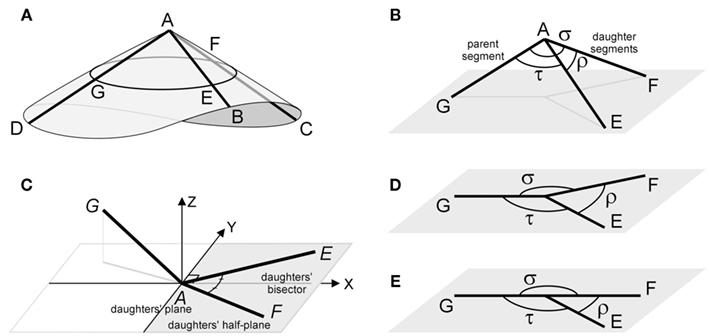
Figure 1. (A) A schematic 3D bifurcation with DA a parent segment and AB and AC the daughter segments. The points G, E, and F on these segments are at unit distance from A. A right circular cone is wrapped around the bifurcation DABC with a circular cross section through G, E, and F. (B) A spatial bifurcation with unit lengths segments, the intermediate angle ρ between the daughter segments, and the side angles σ and τ, between the parent and each of the daughter segments, respectively. (C) An aligned bifurcation with the daughter segments defining the daughter plane (X–Y plane) and the daughters’ bisector coinciding with the positive X-axis. The daughter half-plane contains the daughter segments and is bounded by the Y-axis. (D–E) Two examples of flat bifurcations.
The present study aimed at investigating whether these optimal conditions also apply to neuronal arborizations, in particular to the bifurcations in basal and apical dendritic branching patterns; thus answering the question whether these bifurcations are planar and how parent and daughter segments are oriented with respect to each other.
For practical application, it is convenient to express the measure(s) for flatness of a spatial bifurcation as a function of the three angles determining the bifurcation. We have proposed earlier a measure for flatness, i.e., the cone angle of a bifurcation with only the three bifurcation angles as parameters (Uylings and Veltman, 1975; Uylings and Van Pelt, 2002) and have reported cone angle results for some cortical pyramidal neurons (e.g., Uylings and Smit, 1975), but so far we did not publish formally the derivation of this cone angle. Because of recent renewed interest in this spatial measure by other research groups (Kim et al., 2009), we provide in this paper the derivation in terms of the bifurcation angles. We discovered, however, some shortcomings in the cone angle as measure of flatness of 3D bifurcations (see Discussion) and as, to our knowledge, flatness measure studies have not been published in the past, we developed additional measures and evaluated their properties for quantifying flatness and orientation of 3D bifurcations.
In order to evaluate the various measures for their ability to capture the flatness of 3D bifurcations, they have been applied to sets of random 3D bifurcations and to sets of bifurcations from rat cortical pyramidal cell basal and apical dendrites. Distributions of flatness measures for random and dendritic bifurcations were compared with each other and tested for their differences by means of the Kolmogorov–Smirnov (KS) test. Dendritic and random bifurcations appear to have significant different flatness measure distributions, resulting in the conclusion that dendritic bifurcations do not have randomly oriented parent and daughter segments, and are significantly more flat than random bifurcations. Apical dendritic bifurcations have even more strict planar geometries than basal dendritic bifurcations. This was expected since apical bifurcations are typically “side-branching bifurcations,” a subset of bifurcations with one daughter segment to be a continuation of the parent segment and the other daughter segment to be a side-branch (e.g., by a postponed bifurcation during development). “Side-branching bifurcations” have theoretically a planar configuration, since a plane is defined by two non-identical lines.
The dihedral angle β, i.e., the angle between the daughters’ half-plane (Figure 1C) and the plane formed by the parent segment and the boundary line of the daughters’ half-plane (Figure 1C), appeared to be the most discriminative and interpretable flatness measure and is, therefore, proposed as the first choice for quantifying the flatness of spatial bifurcations. The distributions of the parent azimuth angle and the parent stretch angle show that in basal dendritic bifurcations the parent segment has a strong tendency to be oppositely aligned to the daughters’ bisector.
Materials and Methods
Characteristics of a 3D Bifurcation
A 3D bifurcation DABC is defined by three segments DA, BA, and CA connected at a bifurcation point (apex A; Figure 1A). Without restricting generality we will study spatial bifurcations with equal segment lengths AE = AF = AG (Figure 1B) and distinguish GA as the parent segment and AE and AF as the daughter segments. The tips on the parent and daughter segments are, looking from the inside of the bifurcation, assigned in the order G, E, F. The spatial configuration is determined by the three bifurcation angles between the segments and we distinguish (Figure 1B) the intermediate angle ρ between the daughter segments AE and AF, the side angle σ between daughter segment AF and parent segment AG, and the side angle τ between daughter segment AE and parent segment AG. The bifurcation angles ρ, σ, and τ are then ordered in a clockwise rotation seen from the inside of the bifurcation.
Both daughter segments define the daughters’ plane (Figure 1C). The bisector of the intermediate angle will be called the daughters’ bisector. The daughters’ half-plane is the part of the daughters’ plane containing the daughter segments and bounded by the line through the bifurcation point perpendicular to the daughters’ bisector (Figure 1C). The chosen coordinate system has its X-axis aligned with the daughters’ bisector, its Y-axis aligned with the boundary line of the daughters’ half-plane and its Z-axis orthogonal to the daughters’ plane.
Measures of Flatness of a 3D Bifurcation
Various measures of flatness of 3D bifurcations have been developed for their quantification. For practical application, we have expressed these measures mathematically in terms of the bifurcation angles ρ, σ, and τ, or in terms of the quantities r = 1 − cos ρ, s = 1 − cos σ, and t = 1 − cos τ. A summary of these measures and their expressions is given in Figure 2, together with illustrative pictures. Full derivations of the expressions are presented in the Section “Appendix.” A short description of the measures is given in the next paragraphs.
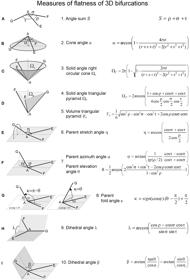
Figure 2. Summary of measures used for quantifying the flatness of 3D bifurcations. The measures are named in the second column with illustrative pictures of how they are defined in the first column. The third column presents the mathematical expressions of the flatness measures in terms of the bifurcation angles ρ, σ, and τ (A) or in terms of the quantities r = 1 − cos ρ, s = 1 − cos σ, and t = 1 − cos τ. (A) A 3D bifurcation with parent segment GA bifurcating at node A into two daughter segments AE and AF. The Angle Sum sums the three bifurcation angles between the segments, denoted by ρ, σ, and τ, (B) Cone angle α as the apex angle of the right circular cone enwrapping a 3D bifurcation, (C) Solid angle ΩC of the right circular cone, (D) Solid angle ΩP and Volume VP of the triangular pyramid, (E) Parent stretch angle η between the parent segment and the bisector of the daughter segments, (F) Azimuth angle φ and Elevation angle θ of the Parent segment in an aligned bifurcation, (G) Parent fold angle κ between parent segment and (the extension of) its projection in the daughter’s half-plane, (H) Dihedral angle λ between the planes formed by the parent segments and each of its daughter segments, and (I) Dihedral angle β between the daughter’s halfplane and the plane formed by the parent segments and the perpendicular to the daughter’s bisector in the daughters halfplane. This dihedral angle β was found to be the preferred measure of flatness of 3D dendritic bifurcations.
Sum of the three bifurcation angles
A measure for flatness of a 3D bifurcation is the sum of the three bifurcation angles (Figure 2A), S = ρ + σ + τ. The value domain of the angle sum S ∈ [0, 2π]. When the angle sum is equal to 2π, then the bifurcation is planar (Figure 1D). When one of the bifurcation angles is equal to 180°, the bifurcation is planar, since a plane is defined by two non-identical lines (Figure 1E).
Cone angle α of right circular cone
The right circular cone circumscribing a 3D bifurcation is obtained by constructing a circle through the tips G, E, and F which are at equal distances from the bifurcation point A (Figure 1A). The apex angle of the right circular cone is called cone angle α (Figure 2A). Its expression in terms of the bifurcation angles is given in “Derivation of Cone Angle, i.e., Apex Angle of the Right Circular Cone Circumscribing a 3D Bifurcation” in Appendix. The cone angle α has a value domain α ∈ [0°, 180°]. The bifurcation is planar for α = 180° (Figure 2B).
Solid angle ΩC of right circular cone
Its expression in terms of the bifurcation angles is given in “Solid Angle of a Right Circular Cone Enwrapping a 3D Bifurcation” in Appendix. The solid angle ΩC of a right circular cone has as value domain ΩC ∈ [0°, 360°]. The bifurcation is planar for ΩC = 360° (Figure 2C).
Solid angle ΩP of triangular pyramid
A 3D bifurcation defines a triangular pyramid with the bifurcation point as apex and the tips of its segments defining the planar base triangle (Figure 4). The solid angle ΩP is expressed in terms of the bifurcation angles in “Solid Angle of a Triangular Pyramid Formed by a 3D Bifurcation” in Appendix. The solid angle ΩP of the triangular pyramid has as value domain ΩC ∈ [0°, 360°]. The bifurcation is planar for ΩP = 360° (Figure 2D).
Volume VP of the triangular pyramid
The volume of a triangular pyramid is expressed in terms of the bifurcation angles in “Volume of the Triangular Pyramid” in Appendix. The volume of the triangular pyramid with unit length segments has as value domain VP ∈ [0, 1/6]. The bifurcation is planar for VP = 0 (Figure 2D).
Parent stretch angle η
The stretch angle η is defined as the angle between the parent segment and the bisector of the intermediate angle, i.e., daughters’ bisector. The stretch angle η is expressed in terms of the bifurcation angles in “Stretch Angle η, i.e., Angle Between Parent Segment and Bisector of the Intermediate Angle” in Appendix. The stretch angle η has as value domain η ∈ [0°, 180°]. The bifurcation is planar for η = 180°, when the parent segment is oppositely aligned to the daughters’ bisector. For values η ≠ 180°, the parent segment may attain an infinite number of rotational positions around the X-axis (daughters’ bisector). In only two of these positions the parent is in the daughter’s plane, making the bifurcation planar (see also Discussion; Figure 2E).
Parent azimuth angle φ and elevation angle θ
The spherical coordinates (θ, φ) of the parent segment are taken in an aligned 3D bifurcation, with the daughter segments in the X–Y plane, the daughters’ bisector aligned to the positive X-axis, and the parent segment pointing in positive Z-direction. Both coordinates (θ, φ) can be expressed in terms of the bifurcation angles as given in “Parent Azimuth Angle φ, Elevation Angle θ and Fold Angle κ” in Appendix. The parent elevation angle θ has as value domain þeta ∈ [0°, 90°]. The azimuth angle has as value domain φ ∈ [0°, 360°]. The bifurcation is planar for þeta = 0°. For φ = 180° the extrapolation of the parent’s projection coincides with daughters’ bisector making the bifurcation a symmetrical one, i.e., the both side angles are equal (Figure 2F).
Parent fold angle κ
The parent fold angle κ is introduced as a single measure derived from the parent azimuth and elevation angle, in order to combine both flatness and orientation information. It measures the angle between the parent segment and (the extension of) its projection in the daughters’ half-plane as given in “Parent Azimuth Angle φ, Elevation Angle θ, and Fold Angle κ” in Appendix. The fold angle κ is equal to the elevation angle θ when the parents projection is in the daughter’s half-plane, thus when cos φ > 0 (Figure A7) (Expression of the Azimuth Angle φ in Terms of the Bifurcation Angles ρ, σ, and τ). The fold angle κ is equal to the supplement 180° − θ when the parents projection is outside the daughter’s half-plane, thus when cos φ < 0 (Figure A7) (Expression of the Azimuth Angle φ in Terms of the Bifurcation Angles ρ, σ, and τ). The fold angle κ has as value domain κ ∈ [0°, 180°]. The bifurcation is planar for κ = 0° and for κ = 180°. For φ = 180° the extrapolation of parent’s projection coincides with daughters’ bisector and the bifurcation is a symmetrical one, i.e., the both side angles are equal (Figure 2G).
Dihedral angle λ
The dihedral angle λ measures the angle between the planes formed by the parent segment and each of the daughter segments. The dihedral angle λ is derived in “Dihedral Angle λ Between the Planes Formed by the Parent and Each of the Daughter Segments” in Appendix. The dihedral angle λ has as value domain λ ∈ [0°, 180°]. The bifurcation is planar for λ = 0° when both planes are folded in, and for λ = 180° when both planes are folded out (Figure 2H).
Dihedral angle β
The dihedral angle β is the angle between the daughters’ half-plane and the plane formed by the parent segment and the line perpendicular to the daughters’ bisector through the bifurcation point A in the daughters’ plane. The dihedral angle β is derived in “Dihedral Angle β Between the Daughters’ Half-plane and the Plane Determined by the Parent Segment and the Line Perpendicular to the Daughters’ Bisector at the Bifurcation Point” in Appendix, and expressed in terms of the bifurcation angles through (A31) and (A34). The dihedral angle β has as value domain β ∈ [0°, 180°]. The bifurcation is planar for β = 0° when both planes are “folded in,” and for β = 180° when both planes are “folded out” (Figure 2I).
Results
Important for the evaluation of the different flatness measures are their distributions for random bifurcations, which will be used as templates for comparison with the distributions of these measures in natural 3D dendritic bifurcations.
Distributions of Measures of Flatness of Random 3D Bifurcations
Random 3D bifurcations are bifurcations composed of three independent spatially random vectors from a given bifurcation point, with one vector assigned as parent segment and the other two assigned as daughter segments. Random oriented vectors in 3D from a given point can be obtained by taking a vector to a randomly selected point on a sphere centered at that point or, alternatively, by taking random spherical coordinates (θ, φ). For random orientations the azimuth angle φ is uniformly distributed over the interval [0, 2π], and a random azimuth angle is obtained by φrand = x.2π with x a uniform random number on the interval [0, 1]. The elevation angle θ of random oriented vectors is distributed as 0.5 cos θ (see Probability Distribution of the Elevation Angle θ of Random Bifurcations with  and with a cumulative distribution
  A random elevation angle is obtained by taking
  with x a uniform random number on the interval [0, 1]. Then, sin θrand = 2x − 1, and

For most of the flatness measures, analytical expressions for the shape of the distributions for random 3D bifurcations were obtained, except for the measures “angle sum” and “solid angle triangular pyramid.” In addition, distributions for 3D random bifurcations of all the flatness measures were obtained by applying them to large sets of generated 3D random bifurcations.
Probability distribution of the bifurcation angles
Without restriction of generality we may align a pair of two random vectors such that one of them coincides with a given direction, say the Z-axis. The question of the angle distribution between two random vectors is then similar to the question of the angle distribution between a random vector and the positive Z-axis. The endpoints of random vectors with length R are uniformly distributed on a sphere with radius R. All the vectors with a given angle δ with respect to the Z-axis have their end points on a certain circle of that sphere (see Figure 3).
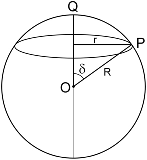
Figure 3. Angle δ between a random vector OP and a given vector OQ. All random vectors with an angle δ with respect to OQ end at the circle with radius r.
The probability of having a random point on the sphere being positioned on the circle with radius r is proportional to its circumference, thus

Probability of having a random point on the sphere is proportional to the integral
Thus the probability of an angle δ between two random vectors is equal to

The three bifurcation angles ρ, σ, and τ are thus distributed according to p(δ), with

Probability distribution of the sum of the three bifurcation angles in a random 3D bifurcation
Bifurcation angles in 3D bifurcations as well as their sum S have restrictions in the values they can adopt: (i) bifurcation angles are each smaller than or equal to 180°, (ii) the largest bifurcation angle is smaller than or equal to the sum of the other two bifurcation angles, and (iii) the sum S of the three bifurcation angles is smaller than or equal to 360°. In order to obtain the distribution function for the sum of the three bifurcation angles, we first derived the one for the sum v of two bifurcation angles resulting in
with v the sum of two bifurcation angles, say ν = σ + τ, with σ ∈ [0, π], τ ∈ [0, π], and ν ∈ [0, 2π]. It is easy verified that for positive x, p2(π − x) = p2(π + x), showing the symmetry of the distribution p2(v) around angle v = π. The distribution function for the sum of the three bifurcation angles could, however, not be obtained in a closed expression. We arrived at the final convolution integral equation
with S the sum of the three bifurcation angles S = ρ + σ + τ = ρ + v, with ρ ∈ [0, π], σ ∈ [0, π], τ ∈ [0, π], v ∈ [0, 2π], S ∈ [0, 2π], and p1(x) = 0.5 sin x. Rather than solving Eq. 7 numerically, the distribution for the bifurcation angle sum has been obtained by generating 1000000 random bifurcations as described in Section “Distributions of Measures of Flatness of Random 3D Bifurcations,” and calculating the sum of the three bifurcation angles. The derivation of the expressions for both distributions is accessible as supplementary material at http://www.bio.vu.nl/enf/vanpelt/papers/VanPelt_Uylings_2012_Supplementary_Material.pdf.
Probability distribution of the cone angle α of random bifurcations
The cone angle α is defined as the angle of the right circular cone circumscribing the 3D bifurcation (Figure 2B), with α ∈ [0, π]. The shape of the cone angle probability distribution has recently been derived by Kim et al. (2010) to be

A short route to this distribution equation follows from the fact that any triangle with its three points on the circle with radius r (Figure 4) results in a cone with the same cone angle α.
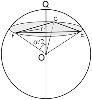
Figure 4. All triangles with points on the circle with radius r define the same right circular cone with cone angle α.
The probability that a random vector has an angle α/2 with a given line OQ is equal to pV(α/2|OQ) = 0.5 sin(α/2) (Eq. 4). The probability of having three points on the circle with radius r is thus equal to the probability of having three random vectors with an angle α/2 with respect to OQ (Figure 4), and thus equal to pV3(α/2|OQ). The probability of a cone angle α is thus proportional to

To obtain a normalized probability distribution for α ∈ [0, π] we use the identity

(e.g., Bartsch, 1985) to calculate

giving us the normalized probability for the cone angle α of

This probability is independent of the orientation of OQ and thus proving (8).
Probability distribution of the solid angle of right circular cone ΩC of random bifurcations
The solid angle ΩC is defined as the solid angle of the right circular cone circumscribing the 3D bifurcation (Figure 2C), with ΩC ∈ [0, 2π]. The solid angle of a right circular cone ΩC relates to the cone angle α via (see Solid Angle of a Right Circular Cone Enwrapping a 3D Bifurcation)

and is on the interval α = [0, π] a monotone increasing function of α. The probability distribution of ΩC directly relates to the probability distribution of the cone angle α, given by (8), via

with ΩC1 = 2π(1 − cos α1/2), and ΩC2 = 2π(1 − cos α2/2). With the transformation ΩC = 2π(1 − cos α/2) we have

Thus,

Thus, for the probability density function p(ΩC) we obtain

Probability distribution of the solid angle of pyramid ΩP of random bifurcations
The solid angle ΩP is defined as the solid angle of the triangular pyramid with apex A and the triangle EFG as basis. It measures the area of the part of the unit sphere centered in A and bounded by the base triangle (Figure 2D), with ΩP ∈ [0, 2π]. It was, unfortunately, not yet possible to obtain an analytical expression for this distribution. Therefore, the distribution has been obtained by generating 1000000 random bifurcations as described in Section “Distributions of Measures of Flatness of Random 3D Bifurcations,” and using the equation in Figure 2D for calculating the solid angle of the triangular pyramid.
Probability distribution of parent stretch angle η of random bifurcations
The stretch angle η is the angle between the parent segment and the daughters’ bisector, with η ∈ [0, π], see Figure 2E. For random bifurcations this angle is also distributed as the angle between two random vectors, thus

Probability distribution of the elevation angle θ of random bifurcations
The elevation angle θ is the angle between the parent segment AG and its projection onto the daughters’ plane, with þeta ∈ [0, π/2]), see Figure 2F. It is the π/2-complement of the polar angle χ between the parent segment and the vertical axis

The polar angle χ is distributed as the angle of a random vector with respect to the vertical Z-axis, as derived above. The distribution of the elevation angle θ of a random vector is thus equal to that of the π/2-complement of the polar angle χ. In the case of aligned bifurcations with the parent segment pointing upward with respect to the daughters’ plane the angle interval is restricted to χ ∈ [0, π/2] and the probabilities multiplied with a factor of 2 such that

with χ ∈ [0, π/2] and þeta ∈ [0, π/2].
Note, that without the restriction of positive Z-coordinates the elevation angle would have been distributed as 0.5 cos θ.
Probability distribution of the parent azimuth angle φ of random bifurcations
The parent azimuth angle φ is the angle between the projection of the parent segment onto the daughters’ plane and the daughters’ bisector (Figure 2F). As in random bifurcations the parent segment may have any orientation from the bifurcation point this angle is uniformly distributed on the interval φ ∈ [0, 2π]

Probability distribution of the parent fold angle κ of random bifurcations
The parent fold angle κ is the angle between the parent segment and the line in the daughters’ half-plane through the projection of parent onto the daughters’ plane (Figure 2G). The parent fold angle κ is equal to the parent elevation angle (κ = θ) for cos φ > 0 (when the projection of the parent segment falls in the daughters’ half-plane), and equal to the π-complement of the parent elevation angle (κ = π − θ) for cos φ < 0 (when the projection of the parent segment falls in the complement of the daughters’ half-plane). The parent fold angle is thus defined on the interval κ ∈ [0, π]. The probability distribution is a composite one with a cosine shape for 0 ≤ κ ≤ π/2 and a mirrored one for π/2 < κ ≤ π

Probability distribution of the dihedral angle λ of random bifurcations
The dihedral angle λ is the angle between the planes formed by the parent segment and each of the daughter segments (Figure 2H). While in each of the planes the angle between the parent and the respective daughter is distributed as the angle between two random vectors, the dihedral angle between both planes can still adopt any value and is uniformly distributed on the interval [0, π] as

Probability distribution of the dihedral angle β of random bifurcations
The dihedral angle β is the angle between the daughters’ half-plane and the plane through the parent and the line in the daughters’ plane perpendicular to the daughters’ bisector (Figure 2I). As the parent segment has a random orientation the angle β is uniformly distributed on the interval [0, π] as

Probability distribution of the volume of the triangular pyramid
The volume is calculated for unit lengths of the three segments AE, AF, and AG in Figure 2D. The probability distribution is obtained by generating 1000000 random bifurcations as described in Section “Distributions of Measures of Flatness of Random 3D Bifurcations,” and using the equation in Figure 2D for the volume of the triangular pyramid.
Distributions of measures for flatness of random 3D bifurcations
The frequency distributions for the various measures of flatness, shown in Figure 5, are obtained from the analytical expressions in Section “Distributions of Measures of Flatness of Random 3D Bifurcations,” except for those in Figures 5B,E,L, which have been obtained by simulating 1000000 random bifurcations. Note, that for the other measures distributions were obtained by simulation as well, in order to proof consistency between the “analytical” and “simulated” distributions. The three bifurcation angles at a random bifurcation have equal distributions as they are all defined as angles between two random oriented segments. They are represented inFigure 5A. The bifurcation angle sum distribution (Figure 5B, obtained by simulation) has a complex shape, difficult to interpret from the complex integral Eq. 7. The cone angle distribution (Figure 5C) has a sigmoid-like shape. The solid angle cone distribution (Figure 5D) reflects the cosine function in its Eq. 10. The solid angle of the pyramid (Figure 5E) shows a monotonous decreasing distribution in contrast to the monotonous increasing one for the solid angle of the cone. Both measures thus differ significantly, which finds its origin in the fact that even for three segments with about similar orientations (thus with small pyramid solid angle) the solid angle of the cone can still adopt large values. The parent stretch angle has a sine-shaped distribution (Figure 5F). The parent azimuth angle (Figure 5G) has a uniform distribution. The parent elevation angle has a cosine-shaped distribution (Figure 5H). The parent fold angle distribution (Figure 5I) is a mixture of a cosine-shaped and a mirrored cosine-shaped one. Both the dihedral angle λ (Figure 5J) and the dihedral angle β (Figure 5K) have uniform distributions. The volume of the pyramid (Figure 5L) shows a decreasing distribution with a rapid decline to zero at its maximal volume of 1/6. This value only occurs when the segments are orthogonal to each other. The flatness measures with uniform distributions for random bifurcations (i.e., dihedral angles λ and β) may be advantageous when comparing with experimental distributions. The statistics of the distributions of the various flatness measures for random bifurcations, obtained from the simulated data, are summarized in Table 1.
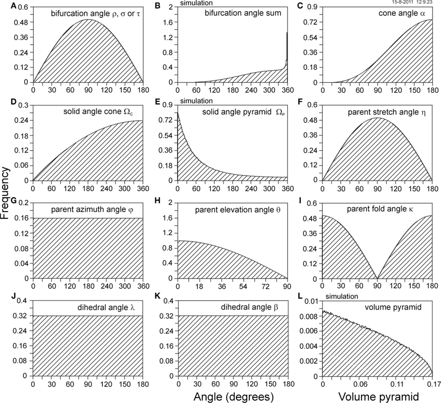
Figure 5. Frequency distributions of the bifurcation angles ρ, σ, and τ in (A) and various flatness measures of 3D bifurcations with segments uniform random oriented in space. All the angle distributions have an angle axis in degrees divided into 180 bins, and are normalized on an angle scale in radians. The distributions are obtained from the analytical expressions, except for those in panels (B,E,L) which are obtained by simulating 1000000 bifurcations. The flatness measures used are (B) the sum of the three bifurcation angles, (C) the right circular cone angle α, (D) the solid angle ΩC of the right circular cone, (E) the solid angle ΩP of the pyramid, (F) the stretch angle η of the parent segment with respect to the daughters’ bisector, (G) the azimuth angle φ of the projection of the parent segment onto the daughters’ plane with respect to the daughters’ bisector, (H) the elevation angle θ of the parent segment with respect to the daughters’ plane, (I) the parent fold angle κ, (J) the dihedral angle λ between the planes formed by the parent segment and each of the daughter segments, (K) the dihedral angle β between the daughters’ plane and the plane through the parent and the line perpendicular to the daughters’ bisector, and (L) the volume of the triangular pyramid (for unit length segments).
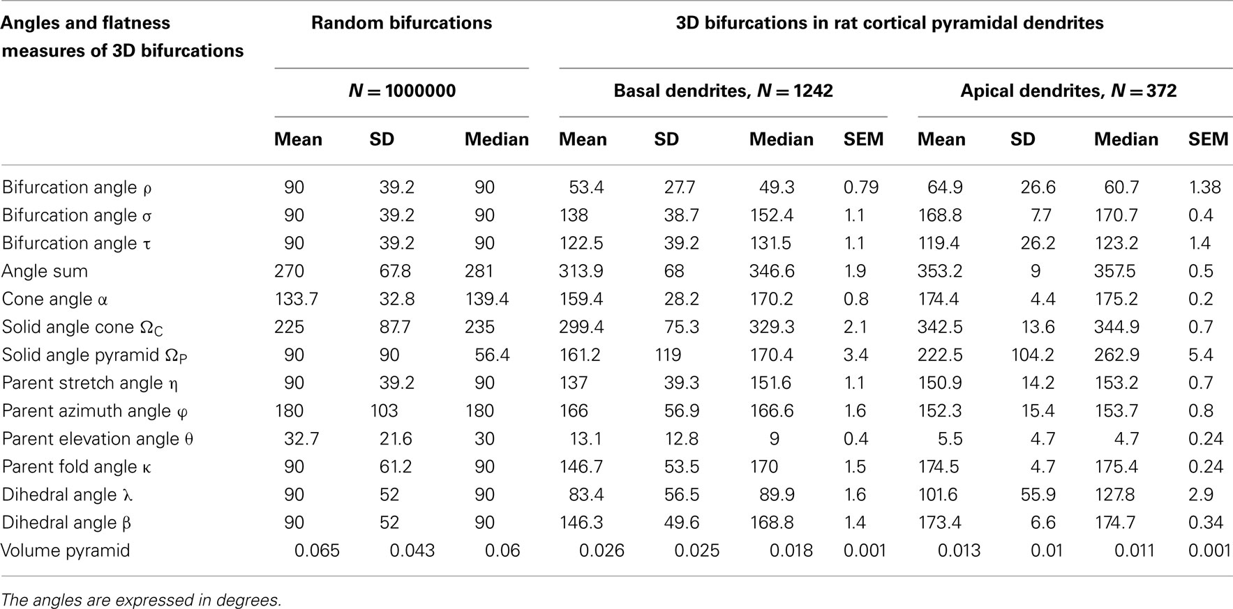
Table 1. Means and SD of characteristic angles (degrees) and flatness measures of 3D bifurcations in a data set of random bifurcations (obtained by simulating 1000000 bifurcations), in rat cortical pyramidal cell basal dendrites (no. of bifurcations 1242), and in apical main stems (no. of bifurcations 372).
Distributions of Measures of Flatness of Bifurcations in Dendrites of Pyramidal Neurons
A set of 112 pyramidal neurons have been obtained from layer III in the visual cortex of six rats. The basal dendritic trees and the apical dendrites have been measured with a semi-automatic 3D tracking system developed by Coleman et al. (1977), see for a further description of these neurons and their analysis Uylings et al. (1978a,b). Apical main stem bifurcations are side-branching bifurcations, in which the side branches are the oblique dendrites. Parent and daughter segments were defined as the connection lines between the bifurcation point and the subsequent bifurcation or end points for the daughter segments and the previous root or bifurcation point for the parent segment. The bifurcation angles were subsequently calculated on the basis of the Cartesian 3D coordinate measurements (Smit and Uylings, 1975). The frequency distributions of the various measures of flatness of the 3D bifurcations are shown in Figure 6 for the basal dendrites (n = 1242) and in Figure 7 for the apical main stem (n = 372). For comparison, the distributions for random 3D bifurcations are included.
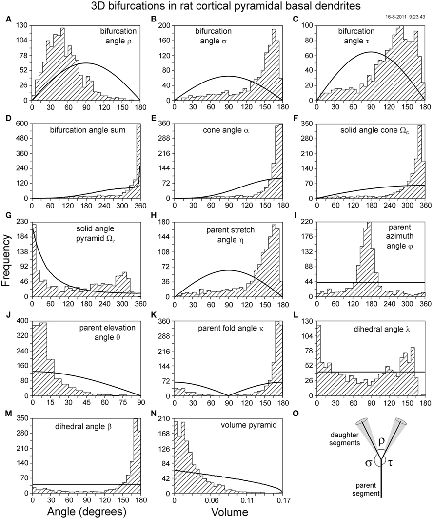
Figure 6. Frequency distributions of various measures of flatness of 3D bifurcations obtained from a data set of 3D reconstructed rat cortical pyramidal basal dendrites (n = 1242), displayed as hashed histograms, and from a number of 1000000 random bifurcations, drawn as solid lines. The horizontal axes display the angles (degrees) of the flatness measures except for (N), displaying a volume (for unit length segments). The hashed histograms are made up of 30 bins, except for (J) which has 15 bins in order to have the same bin width of 6° as (K). The solid lines are based on 100 bins. The statistical outcomes of the distributions are summarized in Table 1. The various panels illustrate the distributions of (A–C) the bifurcation angles ρ, σ, and τ, (D) the sum of the bifurcation angles, (E) the cone angle α, (F) the solid angle ΩC of the right circular cone, (G) the solid angle ΩP of the triangular pyramid, (H) the parent stretch angle η, (I) the parent azimuth angle φ, (J) the parent elevation angle θ, (K) the parent fold angle κ, (L) the dihedral angle λ, (M) the dihedral angle β and (N) the volume VP of the triangular pyramid. (O) Illustrates a symmetrical bifurcation.
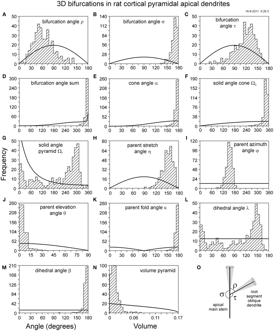
Figure 7. Frequency distributions of various measures of flatness of 3D bifurcations obtained from a data set of 3D reconstructed rat cortical pyramidal apical main stem dendrites (n = 372), displayed as hashed histograms, and from a number of 1000000 random bifurcations, drawn as solid lines. See for (A–N) the legends at Figure 6. (O) Illustrates a side branching bifurcation.
3D bifurcations in pyramidal cell basal dendrites
Bifurcations in basal dendrites have remarkable flat geometries, reflected by the highly skewed distributions of most of the flatness measures. The dihedral angle β (Figure 6M), the parent fold angle (Figure 6K), and the cone angle (Figure 6E) display values close to 180°. The angle sum (Figure 6D) and the solid angle cone (Figure 6F) show values close to 360°. The parent elevation angle (Figure 6J) and the volume of the pyramid (Figure 6N) show highest frequencies at small angles and volumes, respectively. On the other hand, the values for the solid angle pyramid (Figure 6G) and the dihedral angle λ (Figure 6L) still remain broadly distributed, indicating that these measures do not strongly capture the flatness properties of 3D bifurcations. In addition to a flat geometry, parent segments also show a strong alignment opposite to the daughters’ bisector. This can be concluded from the parent azimuth angle distribution peaking around 180° (Figure 6I), and the highly skewed parent stretch angle distribution peaking toward 180°. In addition, bifurcations in basal dendrites have a mean intermediate angle of 53°, significantly smaller than the mean side angles of 123° and 138° (Table 1; Figures 6A–C), respectively. Such geometries result in so-called “symmetrical” bifurcations (Figure 6O). The distributions in Figure 6 also illustrate the variation in the various measures. For instance, the small angle tails in the side-angle distributions indicate that backward oriented daughter segments may occur as well, but with low frequencies. The low frequency “background” in the azimuth angle distributions indicates a small contribution of non-aligned bifurcations. Thus we can conclude that non-optimal backward and ipsilateral bifurcations do occur, but rarely.
3D bifurcations in pyramidal cell apical dendrites
The bifurcations in the apical dendrites are restricted to the side-branching ones of the apical main stem, giving rise to the oblique dendrites. These bifurcations are typically formed by side branching of the apical main stem and have a geometry in which the parent segment and one of the daughter segments are part of the main stem, and the other daughter segment is the root segment of the oblique dendrite (see Figure 7O). Because one of the daughter segments is aligned with the parent segment, one of the side angles (bifurcation angle σ) adopts values close to 180 degrees (Figure 7B), while the other bifurcation angle τ is about the π complement of the intermediate bifurcation angle ρ (Figures 7A,C). In such cases, the bifurcation has a flat geometry, making the apical main shaft side-branching bifurcations theoretically planar. This is reflected in the distributions of the various flatness measures, as the values of the dihedral angle β (Figure 7M), the parent fold angle (Figure 7K), and the cone angle (Figure 7E) show a narrow peak close to 180°, while the angle sum (Figure 7D) and solid angle of circular cone (Figure 7F) show values very close to 360˚. The parent elevation angle (Figure 7J) and the volume of the pyramid (Figure 7N) show highest frequencies at the lowest angles and volumes, respectively. In addition, small angle tails are lacking in the distributions of the angle sums, cone angle, solid angle of circular cone, the parent stretch angle, the fold angle, and the dihedral angle β. Especially the apical main shaft bifurcations demonstrate that the dihedral angle λ (Figure 7L) and the solid angle of the triangular pyramid (Figure 7G) lack the sensitivity to indicate the flatness of planar bifurcations as they maintain even here broad distributions. The root segments of oblique dendrites are slightly oblique oriented (Figure 7O) with typical values for the angle τ of 119° (Table 1). The parent azimuth angle shows an offset of about 28˚ from the value of 180° because the apical main shaft bifurcations are asymmetrical, i.e., daughters’ bisector is not aligned to the apical parent segment.
Comparison of 3D Bifurcations in Pyramidal Cell Dendritic Trees and of Random 3D Bifurcations
Figures 6 and 7 include the distributions for random bifurcations, allowing direct visual comparisons. For most of the flatness measures it is clearly shown that dendritic and random bifurcations differ substantially in their distributions, in most cases without doubt about their significance. In particular, easy visual comparisons were made for the azimuth angle φ and the dihedral angle β, which have uniform distributions for random bifurcations, in contrast to the dendritic ones. Quantitative comparison by means of the KS test (based on the routine “ksone” from Numerical Recipes; Press et al., 1992), confirmed that both basal and apical dendritic bifurcations produce frequency distributions which are significant different from random bifurcations for all the measures used, except for the dihedral angle λ. The differences make clear that dendritic bifurcations are not random but have their branches significantly more oriented in a plane. The various measures of flatness differed in their ability to distinguish dendritic from random distributions. The highest discriminative power (i.e., the maximal difference between dendritic and random cumulative frequency distributions in the K–S test) was shown for the dihedral angle β and the fold angle κ. As the dihedral angle β is also uniformly distributed for random bifurcations, this measure is proposed as the best one to use for determining the flatness of a bifurcation.
Correlations between flatness measures – scatterplots
An important property of the different measures for flatness is how they are related for individual bifurcations. This can be visualized in 2D scatterplots in which for a number of bifurcations the values of two flatness measures are plotted against each other. In Figure 8 the values of various flatness measures are plotted versus the dihedral angle β for basal dendritic bifurcations and for random bifurcations.
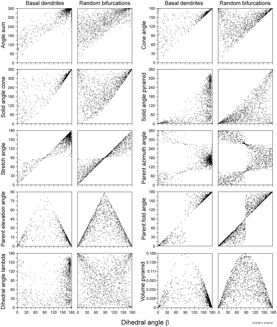
Figure 8. Scatter plots of the various measures of flatness versus the dihedral angle β for the 1242 basal dendritic bifurcations (first and third column) and for a similar number of random bifurcations (second and fourth column). Note, that the frequency distributions of data points along the axes conform to the distributions in Figures 5 and 6 for random and basal dendritic bifurcations, respectively. The data points along the horizontal axis in the random bifurcation panels are thus uniformly distributed and in the basal dendritic bifurcation panels distributed as in Figure 6M.
The scatterplots for the random bifurcations in Figure 8 show how the value domains of the various measures relate to each other, how the density of data points varies over these domains, and how the domain sizes and densities are related.
From the domain boundaries in the scatterplots of Figure 8 can be concluded that (i) the angle sum is generally greater than or equal to twice the dihedral angle β; (ii) the cone angle is greater than or equal to the dihedral angle β; (iii) the solid angle cone is larger than some non-linear function of the dihedral angle β; (iv) the solid angle pyramid is smaller than twice the dihedral angle β; (v) the parent stretch angle adopts values in the region bounded by the diagonal and the horizontal line at 90˚ for the stretch angle; (vi) the parent azimuth angle and dihedral angle β adopt values in three different regions, bounded by vertical line at 90˚ for the dihedral angle β, and the lines at 90˚ and 270˚ for the azimuth angle; (vii) the parent elevation angle is smaller than or equal to the dihedral angle β or its π-complement; (viii) the parent fold angle and dihedral angle β adopt values within areas bounded by the diagonal and the vertical line at 90˚ for the dihedral angle β; (ix) the dihedral angle λ and dihedral angle β do not show domain boundaries; and (x) the volume of the pyramid has its maximum of 1/6 at 90˚ for the dihedral angle β, and decreases steeply for smaller and large angles of β.
Because the values for the dihedral angle β are uniformly distributed on the domain [0˚, 180˚] (Figure 5K), an equal number of data points within each dihedral angle interval in a scatterplot has to be distributed over a varying domain size and in a specific pattern for the other measure, resulting in complex variation in densities of data points. The optimality constraints in basal dendritic bifurcations add additional variation in densities of data points in these scatter plots, resulting in striking differences between the random and dendritic panels.
Only the parent elevation angle and azimuth angle are orthogonal measures and independent for random bifurcations. This is shown in Figure 9 (right panel) where the random bifurcation data points are uniformly distributed along the parent azimuth angle axis and cosine distributed along the parent elevation angle axis. The basal dendrite data points (left panel), however, are strongly clustered at small elevation angles and around 180˚ azimuth angle. This Figure most clearly shows how basal dendrite bifurcations differ from random ones. The small elevation angles of parent segments versus their daughters’ plane demonstrate the flatness of the basal dendritic bifurcations. The azimuth angles around 180˚ demonstrate the opposite alignment of the parent segment versus the daughters’ bisector in basal dendritic bifurcations. While most of the dendritic bifurcation data points are located in the cluster, some have a wider spread, with parent elevation angles still remaining smaller than about 50˚, but with parent azimuth angles spreading out over their whole domain (see also Figures 6I,J). Thus a minority of dendritic bifurcations outside the central cluster show lack of alignment with respect to the daughters’ bisector with for a few of them slightly increased parent elevation angles.
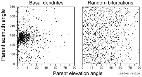
Figure 9. Scatter plots of the parent azimuth angle versus parent elevation angle values for basal dendrite bifurcations (left panel) and random bifurcations (right panel).
Summary, Discussion, and Conclusion
Flatness of 3D Dendritic Bifurcations
The flatness of 3D bifurcations in neuronal (dendritic) arborizations was investigated in order to test the hypothesis that these bifurcations are more planar than random ones, caused by some optimality principle. A number of different measures of flatness have been derived and applied to bifurcations of rat cortical pyramidal basal and apical dendrites (Uylings et al., 1978a,b) and to random bifurcations. The measures have been evaluated for their ability to optimally describe the flatness properties of 3D bifurcations.
The various flatness measure distributions showed quite distinct shapes, ranging from uniform ones to highly skewed, or even bimodal ones. In particular the flatness measures with uniform distributions for random bifurcations were interesting for the ease of comparison with experimental distributions. These were the parent azimuth angle φ, the dihedral angle λ, and the dihedral angle β.
Almost all flatness measures, except for the dihedral angle λ, show that parent and daughter branches in dendritic bifurcations have a strong tendency to be oriented in a flat plane. Basal dendritic flatness measure distributions still show some low frequency background, indicating deviations from strict planarity. Apical bifurcations, however, do not show such background, indicating that they are much less variable in flatness. The distributions of the azimuth angle and stretch angle indicate a preference for basal dendritic bifurcations to be symmetrical, i.e., with the parent segment oppositely aligned with the daughters’ bisector. Apical bifurcations, however, are not symmetrical as they originate from side branching from an apical main stem, thus having an apical parent segment oppositely aligned with one of the daughters (the apical daughter segment). Apical main stem and side branch thus form already geometrically one plane. Such is not trivial for basal dendritic bifurcations when both daughter branches still need to find their orientation after a branching event at the parent segment.
Among the scatter plots it was the one with the spherical coordinates (θ, φ) that displayed the most clearcut information about the existence of symmetrical bifurcations and thus the opposite alignment of the parent segment with respect to the daughters’ bisector. The parent fold angle was actually introduced to combine the information in the spherical coordinates pair into one single measure. Indeed, together with the dihedral angle β, it was the most discriminative measure in the K–S test comparison of random and dendritic bifurcations. The dihedral angle β measure has the advantage to be uniformly distributed for random bifurcation, in contrast to the double cosine-shaped distribution for the parent fold angle. Therefore, the flatness measure that best described the difference between dendritic and random distributions is selected to be the dihedral angle β.
Kim et al. (2009, 2010) used the cone angle to analyze the bifurcations in different cell types and found it peaking at 180˚. Their analysis of random bifurcations (obtained by a different approach than in the present paper) also showed a peak at 180˚, making them to conclude that local planar dendrites are the natural result of connecting to the closest point in space, i.e., their procedure to get random bifurcations. The present study has also shown that both neuronal bifurcations and random ones have cone angle distributions, with maximal frequencies at 180˚. However, both the experimental and random distributions differ significantly in their shape (K–S p-value < 0.0001), as is observed in the sharp peak for the observed ones at high cone angle values, and the sigmoidal shape of the random curve.
The intermediate angle between the daughter branches at basal dendritic bifurcations differs significantly in its left-skewed distribution [Mn(SD; SEM) = 53.4(27.7; 0.79)] from the symmetrical distribution for random bifurcations [Mn(SD) = 90(39.2)]. In a detailed study of the architecture of dendritic trees of Cat alpha motoneurons, Marks and Burke (2007) found a similar left-skewed distribution for the angle between daughter branches (called dInterDau in their paper). From Figure 6C in their paper we estimated a mean value 50.7 and a SEM value of 2.2. With the number of observations of 887 an estimate for the SD was obtained of 29.8. The distribution of intermediate angles thus shows striking similarity between cat motoneuron dendrites and rat cortical pyramidal basal dendrites.
Scorcioni et al. (2004) analyzed a large data set of rat hippocampal pyramidal cells and made a systematic analysis of the differences between CA1 and CA3 neurons and of the differences between reconstructing laboratories, using an extensive set of 30 morphometric parameters. Among these were the local and the remote bifurcation angles (intermediate angles in our terminology), measuring the angle between the daughter branches up to their first measured points, or up to their first nodes, respectively. For the remote intermediate angles mean values for the different groups were observed in the range of (44–60), thus showing good agreement with the outcomes of the present report and those of Marks and Burke (2007). They all significantly differed from the random bifurcation prediction. For the local intermediate angles, however, mean values were reported in a much wider range of (54–89). An important finding of this study was that laboratory-specific variabilities were of the same order of magnitude as the cell class-specific ones, and significantly greater than the intrinsic variabilities, while differences among laboratories were largely due to local variables such as local bifurcation angles. Apparently, the choices made during reconstruction close to bifurcation points introduce much variability, making comparisons harder.
Dendritic segments show curviness and the orientation of the proximal parts of the segments to the bifurcation point may differ from their more distal parts. Smit and Uylings (1975) showed, however, that the orientation distributions of the proximal and distal parts have equal mean values but differ somewhat in the SD values.
The opposite alignment of the basal parent segment to the daughters’ bisector (symmetrical bifurcation) supports the hypothesis that the local geometry of a bifurcation during its formation is governed by forces in the parent and daughter branches. The existence of elastic forces in neurons cultured in vitro was already established in the eighties (e.g., Bray, 1979; Dennerl et al., 1988, 1989; Lamoureux et al., 1989; Heidemann et al., 1990). Bray (1979) in particular showed that the angles at bifurcations conformed to those expected from force equilibrium. These cultured neurons, however, grew over flat substrates, thus adopting naturally a flat geometry. The present study has demonstrated that bifurcations in 3D dendritic arborizations also adopt a highly flat geometry which is expected when also in 3D elastic tension in neurites governs local bifurcation geometry. Bifurcations may develop force equilibrium when the distal parts of the branches are anchored to the substrate. Such conditions may be present during and shortly after a branching event by the tension exerted by the daughter growth cones and may govern the “local” bifurcation angles. Further elongation of the daughter branches will go with fluctuations in outgrowth directions and thus in curviness of the branches (Katz, 1985). When the daughter branches bifurcate on their turn or terminate, the “remote” angles between the straight connection lines may show additional variation superposed on the “local” bifurcation angles. When this is a major factor we would expect a higher variability in the values of “remote” or “far” angles. This is not found by Smit and Uylings (1975) and Scorcioni et al. (2004). Another source of variation (perhaps the major one) is the measurement error, which can be assumed to be smaller for remote bifurcation angles than for local ones. Outgrowing daughter branches may change their direction of outgrowth, for instance, when encountering obstacles. The more or less uniform background in the parent azimuth angle distribution (Figure 6I) may very well originate from such events. “Local” bifurcation angles may not show such background in the parent azimuth angle distribution, and may be expected to result in similar of even stronger outcomes concerning bifurcation flatness and parent alignment to the daughters’ bisector.
Evaluation of Measures of Flatness
Some additional findings of the various measures will be discussed in the next paragraphs.
Sum of 3 bifurcation angles: A measure for flatness?
The sum of the three bifurcation angles S = ρ + σ + τ (Figure 1B) may seem a simple measure for flatness of a 3D bifurcation. This variable varies between 0 and 2π. A planar bifurcation, however, reaches the 2π value for this variable, when both side angles are between π/2 and π, and the daughter segments are not ipsilaterally from the parent segment (Figures 10A–C). When the side angles are smaller than π/2, i.e., a recurrent configuration, which is non-optimal (e.g., Figure 10E), the angle sum is not indicative for flatness. Adaptations for the angle sum can be made for these non-optimal cases if the bifurcation is planar. For 3D bifurcations, however, this is not straightforward. When the extrapolation of parent branch vector GA and its projection on the daughter plane lies outside the intermediate angle ρ, the two daughter segments branch ipsilaterally from the parent segment, which is a non-optimal configuration (e.g., Figures 10D, Figures A3 and A9 in Appendix). In such a condition the angle sum S = ρ + σ + τ cannot reach the value of 2π, even when the bifurcation lies in a flat plane. Thus, the sum of 3 bifurcation angles is not an appropriate measure for flatness.
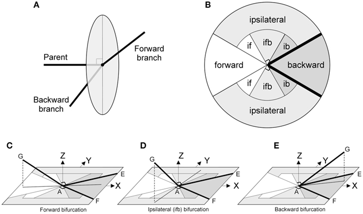
Figure 10. Spatial configurations for forward and backward, and ipsilateral bifurcations. Backward and ipsilateral bifurcations are non-optimal configurations. (A) Viewing from the parent segment: if a side angle is smaller than 90˚, then the pertinent daughter segment runs backward. Bold lines indicate the parent and daughter segments. The circular disk displays the plane perpendicular to the parent segment. When both side angles are equal or larger than 90˚ then both parent segments run in the “forward” half-space and they are not-recurrent, see also (C). (B) This illustrates the situations seen from the daughter segments (bold lines), thus here the parent segment can vary in any direction. When the extrapolation of parent segment and its projection is outside the intermediate angle, the two daughter segments branch ipsilaterally from the parent segment (B,D), else they branch bilaterally (C,E). The intermediate angle is the angle between the daughter segments. The size of the sectors shown depends on the size of the intermediate angle: if: ipsilateral bifurcation with 2 forward running daughter segments; ifb: ipsilateral bifurcation with one backward running daughter segment; ib: ipsilateral bifurcation with 2 backward running daughter segments. (C) A bilateral forward bifurcation. (D) An ipsilateral bifurcation with one backward and one forward running daughter segment (indicated by “ifb”). (E) Both daughter segments run backward, specified by “backward” in (B), bilateral configuration.
Cone angle α and solid angle ΩC of a right circular cone
A solid angle is the part of space bounded by straight lines extending from a single point to a subtending closed curve or polygon. Thus the solid angle is a measure for 3D space from an apex contained in a 3D object, e.g., a cone apex at the center of a sphere. The solid angle is usually expressed in steradians (sr) and is considered to be dimensionless in mathematics and physics, just like radians or degrees of an angle. For a right circular cone circumscribing a 3D bifurcation holds, that each cone angle value corresponds only with one particular value of its solid angle, ΩC, see Eq. A14. The cone angle and the solid angle of the right circular cone circumscribing a 3D bifurcation give maximal values for maximal flatness of a bifurcation, i.e., π radians and 2π steradians, respectively, and reach the minimal value 0 for minimal flatness. However, bifurcations may have large cone angles or solid angles, but still have “pathological”/non-optimal configurations. For instance, Figure A3 in Appendix illustrates a bifurcation with a large cone angle, but still a non-optimal one with small bifurcation angles (crystal-needle-like structure) and daughter segments turning back in the direction of the parent segment. Thus as specified in Introduction we need to take into account the values of side angles: thus next to the spatial measure of cone angle or solid angle of right circular cone we need to know whether both side angles are between π/2 and π, and the projection of the extrapolation of the parent branch is within the intermediate angle (Figure 10).
Solid angle ΩP of triangular pyramid
The solid angle for a triangular pyramid with apex A (Figure 2C, Figure A4 in Appendix), also called the trihedral angle (Polyanin and Manzhirov, 2007), is expressed by van Oosterom and Strackee (1983) as a function of the vector position and the size of the three edges of the triangular pyramid, e.g., the parent and daughter segments of a 3D bifurcation. We defined the trihedral angle in terms of the three planar bifurcation angles, see Eq. A20. There is no straightforward relation between the trihedral angle and the solid angle of a circular cone, since one particular solid angle ΩC contains an infinite number of 3D bifurcations with its node at the apex having different values for solid angle of triangular pyramid which range between 0 < ΩP < ΩC. Three-dimensional bifurcations with a very small trihedral angle can be constructed close to a flat plane in a right circular cone with a very wide cone angle close to π radians or a solid angle close to 2π steradians (e.g., pyramids with a very small intermediate angle and wide side angles near π). Flatness of a 3D bifurcation is, thus, a different property than the trihedral angle or a solid angle of triangular pyramid expresses. This is also shown in the value distribution of the solid angle of a triangular pyramid for three spatially random vectors (Figure 5E).
Parent stretch angle η
The stretch angle η varies between 0 and π. It reaches the value π, only when the parent segment is oppositely aligned to the daughter’s bisector. Then, the bifurcation lies in a flat plane. However, there are cases that a bifurcation is planar, but with a value for the stretch angle is ≪π. For instance (case 1), the bifurcation is a side branching, i.e., one side-angle is ∼π and the other side-angle is π/2 or a little larger. A side branching is a planar bifurcation, but in this situation is the stretch angle: ∼(π/2 + π/4),i.e., ∼(3/4 π), thus about 25% lower than π; or (case 2) the bifurcation lies in a flat plane, but the parent segments’ extrapolation lies outside the intermediate angle ρ, the two daughter segments branch ipsilaterally from the parent segment (Figure 10). Then the stretch angle is ≪π. In fact, the stretch angle η reaches only the value π, when the extrapolation of the parent segment coincides with the bisector of the intermediate angle, thus when both side angles are equal, i.e., a symmetrical bifurcation, and between π/2 and π. Thus, stretch angle values close to π do indicate symmetrical bifurcations with a more or less planar geometry, making the measure of interest in relation to symmetrical bifurcations.
Parent fold angle κ
The parent fold angle is derived from the spherical coordinates pair (θ, φ) into a single measure. It is equal to the parent elevation angle θ when the parents projection is in the daughters’ half-plane, but equal to π − θ when its projection is outside the daughters’ half-plane (Figure A9 in Appendix). The fold angle κ thus distinguishes forward and backward orientation of parent segments with respect to the daughter’s half-plane. For random bifurcations it has shown to generate a symmetrical distribution around φ = π (Figure 5I). For dendritic bifurcations, however, the distribution is highly asymmetric because of the “forward” alignment of the parent segments. Together with the dihedral angle β, it was the most discriminative measure in the K–S test comparison of random and dendritic bifurcations.
Dihedral angle β
Also the dihedral angle β was introduced in order to combine flatness and orientation information. While it produced symmetric (even uniform) distributions for random bifurcations it showed highly asymmetric distributions for dendritic bifurcations, also underscoring the forward orientation of parent segments in the latter ones. An interesting feature was that when the daughter segments are non-optimal recurrent, thus when the side angles are small (i.e., <π/2), the dihedral angle β is also small (i.e., <π/2).
Dihedral angle λ
This measure expresses a different feature of spatial bifurcations than expressed by the dihedral angle β. For bifurcations with a small intermediate angle we expect that this measure can have very small angle λ values even in case of near planar bifurcations. When the side angles, however, have very small values, thus when the daughter segments are recurrent and thus the bifurcation is non-optimal, we can have still values near π. This is not possible for the dihedral angle β.
Summarizing Conclusion
Dendritic bifurcations are significantly more flat than random bifurcations. Basal dendritic bifurcations also show a significant alignment of their parent segments oppositely to the bisector of their daughter segments, resulting in “symmetrical” configurations. Among the different measures of flatness, the dihedral angle β was most favorable as it integrated flatness and alignment information and was found to be the most discriminative and interpretable one and is, therefore, proposed as the first choice for quantifying the flatness of dendritic spatial bifurcations. Also the fold angle κ combined flatness and alignment properties, but did not produced uniform distributions for random bifurcations.
We derived geometric measures as a function of the three bifurcation angles for specification of the extent of flatness of a spatial bifurcation. The values of the individual bifurcation angles, furthermore, are of importance to evaluate particular optimality models (e.g., Uylings, 1977a).
Conflict of Interest Statement
The authors declare that the research was conducted in the absence of any commercial or financial relationships that could be construed as a potential conflict of interest.
Acknowledgments
This work was supported by EU BIO-ICT Project SECO (216593), and by NWO-CLS Project NETFORM (635.100.017)
References
Bray, D. (1979). Mechanical tension produced by nerve cells in tissue culture. J. Cell Sci. 37, 391–410.
Casey, J. (1889). A Treatise on Spherical Trigonometry; and its Application to Geodesy and Astronomy with Numerous Examples. University of Michigan Library, Ann Arbor. [Reprinted in 2007 by Scholarly Publishing Office].
Coleman, P. D., Garvey, C. F., Young, J. H., and Simon, W. (1977). “Semiautomatic tracking of neuronal processes,” in Computer Analysis of Neuronal Structures, ed R. D. Lindsay (New York: Plenum Press), 91–109.
Dennerl, T. J., Joshi, H. C., Steel, V. L., Buxbaum, R. E., and Heidemann, S. R. (1988). Tension and compression in the cytoskeleton of PC-12 neurites II: quantitative measurements. J. Cell Biol. 107, 665–674.
Dennerl, T. J., Lamoureux, P., Buxbaum, R. E., and Heidemann, S. R. (1989). The cytomechanics of axonal elongation and retraction. J. Cell Biol. 109, 3073–3083.
Dittmer, H. J. (1937). A quantitative study of the roots and root hairs of a winter rye plant (Secale cereale). Am. J. Bot. 24, 417–420.
Dittmer, H. J. (1948). A comparative study of the number and length of roots produced in nineteen angiosperm species. Bot. Gaz. 109, 354–358.
Donnay, J. D. H. (1945). Spherical Trigonometry After the Cesàro Method. [Reprinted in 2009, Milton Keynes: Lightning Source UK Ltd.].
Haug, H. (1972). Stereological methods in the analysis of neuronal parameters in the central nervous system. J. Microsc. 95, 165–180.
Heidemann, S. R., Lamoureux, P., and Buxbaum, R. E. (1990). Growth cone behavior and production of traction force. J. Cell Biol. 111, 1949–1957.
Kaandorp, J. A., Blom, J. G., Verhoef, J., Filatov, M., Postma, M., and Müller, W. E. G. (2008). Modelling genetic regulation of growth and form in a branching sponge. Proc. Biol. Sci. 275, 2569–2575.
Kim, Y., Sinclair, R., and De Schutter, E. (2009). Local planar dendritic structure: a uniquely biological phenomenon? BMC Neurosci. 10(Suppl. 1), P4. doi: 10.1186/1471-2202-10-S1-P4
Kim, Y., Sinclair, R., and De Schutter, E. (2010). “Why are dendrites locally planar?” Abstract Poster 190.16. 7th FENS Forum of European Neuroscience, July 3–7, Amsterdam.
Lamoureux, P., Buxbaum, R. E., and Heidemann, S. R. (1989). Direct evidence that growth cones pull. Nature 340, 159–162.
Marks, W. B., and Burke, R. E. (2007). Simulation of motoneuron morphology in three dimensions. I. Building individual dendritic trees. J. Comp. Neurol. 503, 685–700.
McMahon, T. A., and Kronauer, R. E. (1976). Tree structures: deducing the principle of mechanical design. J. Theor. Biol. 59, 443–466.
Polyanin, A. D., and Manzhirov, A. V. (2007). Handbook of Mathematics for Engineers and Scientists. Boca Raton: Chapman and Hall/CRC.
Press, W. H., Teukolsky, S. A., Vettering, W. T., and Flannery, B. P. (1992). Numerical Recipes in Fortran, The Art of Scientific Computing, 2nd Edn. New York: Cambridge University Press.
Scorcioni, R., Lazarewicz, M. T., and Ascoli, G. A. (2004). Quantitative morphometry of hippocampal pyramidal cells: differences between anatomical classes and reconstructing laboratories. J. Comp. Neurol. 473, 177–193.
Smit, G. J., and Uylings, H. B. M. (1975). The morphometry of the branching pattern in dendrites of the visual cortex pyramidal cells. Brain Res. 87, 41–53.
Uylings, H. B. M. (1977a). Optimization of diameters and bifurcation angles in lung and vascular tree structures. Bull. Math. Biol. 39, 509–520.
Uylings, H. B. M. (1977b). A Study on Morphometry and Functional Morphology of Branching Structures, with Applications to Dendrites in Visual Cortex of Adult Rats Under Different Environmental Conditions. Ph.D. thesis, University of Amsterdam, Amsterdam.
Uylings, H. B. M., Kuypers, K., Diamond, M. C., and Veltman, W. A. M. (1978a). Effects of differential environments on plasticity of dendrites of cortical pyramidal neurons in adult rats. Exp. Neurol. 62, 658–677.
Uylings, H. B. M., Kuypers, K., and Veltman, W. A. M. (1978b). Environmental influences on the neocortex in later life. Prog. Brain Res. 48, 261–273.
Uylings, H. B. M., and Smit, G. J. (1975). The three-dimensional branching structure of cortical pyramidal cells. Brain Res. 87, 55–60.
Uylings, H. B. M., and Van Pelt, J. (2002). Measures for quantifying dendritic arborizations. Network 13, 397–414.
Uylings, H. B. M., and Veltman, W. A. M. (1975). Characterizing a dendritic bifurcation. Neurosci. Lett. 1, 127–128.
van Elburg, R. A. J., and van Ooyen, A. (2010). Impact of dendritic size and dendritic topology on burst firing in pyramidal cells. PLoS Comput. Biol. 6, e1000781. doi: 10.1371/journal.pcbi.1000781
van Oosterom, A., and Strackee, J. (1983). The solid angle of a plane triangle. IEEE Trans. Biomed. Eng. 30, 125–126.
van Pelt, J., and Uylings, H. B. M. (2002). Branching rates and growth functions in the outgrowth of dendritic branching patterns. Network 13, 261–281.
van Veen, M., and van Pelt, J. (1992). A model for outgrowth of branching neuritis. J. Theor. Biol. 159, 1–23.
Wen, Q., and Chklovskii, D. B. (2008). A cost-benefit analysis of neuronal morphology. J. Neurophysiol. 99, 2320–2328.
Williams, H. R., Trask, R. S., Weaver, P. M., and Bond, I. P. (2008). Minimum mass vascular networks in multifunctional materials. J. R. Soc. Interface 5, 55–65.
Appendix
In the Section “Materials and Methods” a number of measures of flatness of 3D bifurcations were introduced and mathematically expressed in terms of the bifurcation angles ρ, σ, and τ, or in terms of the quantities r = 1 − cos ρ, s = 1 − cos σ, and t = 1 − cos τ of the 3D bifurcation (Figures 1 and 2). In this Appendix the derivation of these expressions will be given. Although most of the mathematics is straightforward, we have experienced the necessity to describe the derivations explicitly for neuroscientists.
Derivation of Cone Angle, I.e., Apex Angle of the Right Circular Cone Circumscribing a 3D Bifurcation
The circumscribing right circular cone is obtained by constructing a circle through G, E, and F which are at equal distances from the bifurcation point A, i.e., AG = AE = AF = l. This circle and the apex A define a right circular cone (Figure A1A), in which the projection M, from A onto the circle plane, is the center of the circle with radius R (Figure A1A,B). The apex angle of this right circular cone is called the cone angle α. With angle GAM equal to α/2, we have,

and using the trigonometric function of half argument we obtain

thus
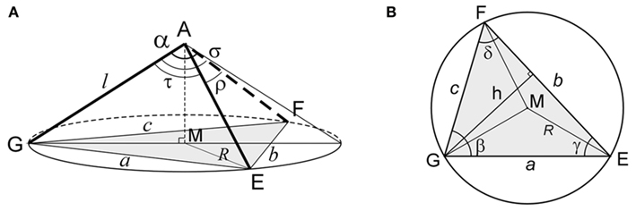
Figure A1. (A) Right circular cone circumscribing a bilateral non-recurrent 3D bifurcation GAEF with its circular base through GEF and cone angle α. M is the projection of the node A onto the circular base, i.e., the center of the circle through GEF. (B) Circumscribed circle of triangle GEF with radius R and center M.
To express the radius R of the circumscribed circle of triangle GEF in terms of the sides a, b, and c of the triangle (Figure A1B), we use the sine rule
and the cosine rule to obtain:

Equating (A4) and (A5) results in:
By defining the semi-perimeter p as p = (a + b + c)/2, (A6) can be rewritten as
Thus, using (A4),

Equation (A8) is known as Heron’s formula (e.g., Polyanin and Manzhirov, 2007).
Inserting (A6) into (A3) yields:
The sides of the triangle can be expressed in terms of the three bifurcation angles of the 3D bifurcation (Figure A1A) with ρ = ∠EAF, σ = ∠GAF, τ = ∠GAE, and using the cosine rule:

Taking r = 1 − cos ρ, s = 1 − cos σ, t = 1 − cos τ, and thus a2 = 2l2t, b2 = 2l2r, and c2 = 2l2s, we obtain for (A9)
and thus
illustrating that the expression for cone angle α is symmetric in r, s, and t, i.e., independent of the order in which r, s, and t are taken. The equations for the cone angle α, given by Uylings and Van Pelt (2002) and Uylings and Veltman (1975), can be derived by substituting
a = 2l·z, b = 2l·x, and c = 2l·y into (A2) and (A6)
in which x = sin(ρ/2), y = sin(σ/2), and z = sin(τ/2):

and after rewriting

Solid Angle of a Right Circular Cone Enwrapping a 3D Bifurcation
The solid angle of a right circular cone enwrapping a 3D bifurcation (and its apex at the bifurcation node) ΩC relates to above-mentioned cone angle α (e.g., Driggers, 2003) as

This relation can be derived as follows
The solid angle of a right circular cone ΩC covering a bifurcation (and with its apex at the bifurcation node) is defined as the surface area of the part of the sphere bounded by the right circular cone divided by the squared radius of the sphere (Figure A2),
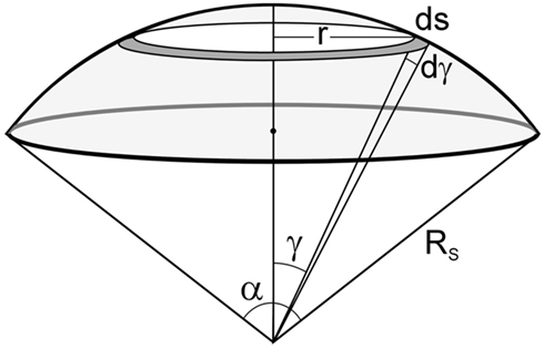
Figure A2. Surface of a sphere viewed from a right circular cone with a cone angle α.
The surface area of this part of the unit sphere can be obtained by integrating the area of a small ring (with radius r) at an angle γ,  over the angle interval [0, α/2]. Thus,
Thus, the solid angle of a right circular cone circumscribing a 3D bifurcation can also be expressed by the three angles defining a 3D bifurcation using (A11) and the trigonometric function of half argument cos2(α/2) = (1 + cos α)/2 as

Equation A3 shows that the cone angle α is fully determined by the radius R of the circumscribed circle for given length l of the segments. An infinite number of different triangles can be drawn within this circle, such that an infinite number of bifurcations will have the same cone angle and solid angle. For instance, Figure A3 illustrates another 3D bifurcation with the same circumscribing right circular cone as displayed in Figure A1A.
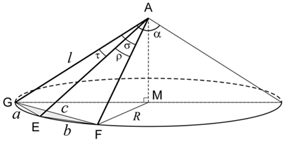
Figure A3. The same circular cone as in Figure A1A, but circumscribing an ipsilateral, recurrent 3D bifurcation, GAEF.
Solid Angle of a Triangular Pyramid Formed by a 3D Bifurcation
A 3D bifurcation defines a triangular pyramid with the bifurcation point as apex and the tips of its branches defining the planar base triangle. By definition the solid angle of a triangular pyramid equals (Figure A4)
with ΔEFG equal to the surface area of the spherical triangle on the sphere through the tips and centered at the bifurcation point and l the radius of the sphere. The surface area of the spherical triangle ΔEFG is equal to ΔEFG = l2ε (e.g., Polyanin and Manzhirov, 2007) and thus

with ε the spherical excess of the spherical triangle EFG. For a spherical triangle with sides e, f, g and angles γ, μ, ν (Figure A4), we have the following relations (e.g., Polyanin and Manzhirov, 2007)

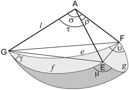
Figure A4. The solid angle of a triangular pyramid formed by equal segments parts l from the node A, of a 3D bifurcation subtends a spherical triangle GEF with spherical center at the apex of pyramid and radius l. The sides of the spherical triangle are denoted by e, f, and g, and its spherical angles by γ, μ, and ν.
Casey (1889, reprinted 2007) has reported an expression for ε/2 for the unit sphere (l = 1), in his Eq. 359 on p. 87, i.e.,
called the Euler’s Formula for one-half of the spherical excess expressed in terms of the sides of the spherical triangle (Donnay, 1945, reprinted 2009). The angles τ, ρ, and σ relate to the unit circle segments f, g, and e, respectively, as

This leads to a simple equation for ΩP in terms of the three bifurcation angles

which shows the symmetry in ρ, σ, and τ in ΩP. Eq. A20 is undefined, when one of the three bifurcation angles is π, in such a condition the bifurcation is planar and thus ΩP = 2π.
For the derivation of Euler’s Formula (A18), Donnay (1945, reprinted 2011) applied the stereographic projections method in combination with Cesàro’s method of “Triangles of Elements.” A derivation of Euler’s Formula based on the approach of Donnay (1945) is made available as supplementary material at http://www.bio.vu.nl/enf/vanpelt/papers/VanPelt_Uylings_2012_Supplementary_Material.pdf.
Volume of the Triangular Pyramid
The volume VP of the triangular pyramid AEFG (Figure A5) is given by

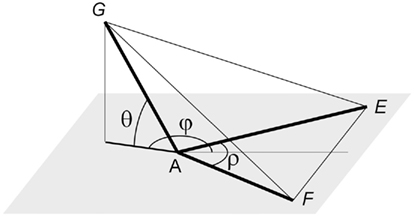
Figure A5. A 3D bifurcation with parent segment AG and daughter segments AE and AF. The orientation of the parent segment is defined by its elevation angle θ with respect to its projection onto the daughter plane and the azimuth angle φ between its projection and the bisector of the angle ρ between the daughter segments.
Given that  [see (A33) below],
it follows that 
and finally

Stretch Angle η, i.e., Angle between Parent Segment and Bisector of the Intermediate Angle
The stretch angle is defined as the angle η between the parent segment and the bisector of the intermediate angle, i.e., daughters’ bisector (Figure A8). Unit lengths are assumed for both parent segment GA and daughter segments AF and AE, respectively.
With the stretch angle η equal to ∠GAH (Figure A6), and GH the median to EF, we derive from the squared length of median GH and the law of cosine:

in which GF2 = 2(1 − cos σ), GE2 = 2(1 − cos τ), EF2 = 2(1 − cos ρ), and AH = cos ρ/2.
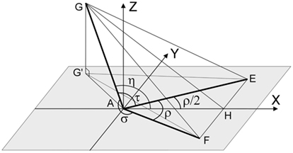
Figure A6. An aligned spatial bifurcation GAEF with stretch angle η between parent segment and the bisector AH of the intermediate angle ρ.
Thus

and
resulting in
Equation A24 is not symmetrical in the bifurcation angles ρ, σ, and τ due to the choice of defining the stretch angle between the parent segment and the bisector of bifurcation angle ρ. Eq. A24 is undefined for intermediate angle ρ = π, but then the bifurcation is planar and we define η = π.
Parent Azimuth Angle φ, Elevation Angle θ, and Fold Angle κ
The spherical coordinates of the parent segment AG in the aligned bifurcation are given by the parent elevation angle θ, measuring the angle between the parent segment AG and its projection AG′ onto the daughter plane, and the azimuth angle φ between daughter’s bisector (X-axis) and the parent’s projection AG′ onto the “daughters” plane’ (Figure A7). The fold angle κ is derived from the azimuth and elevation angle, and combines both flatness and orientation information. It measures the angle between the parent segment and (the extension of) its projection in the daughters’ half-plane (see Figure A7)

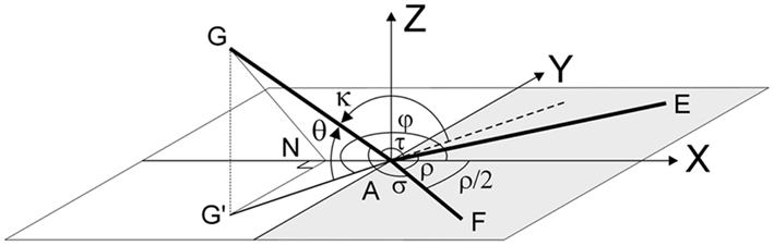
Figure A7. The fold angle κ, i.e., angle between parent segment and the half-plane determined by the two daughter segments, is in this spatial non-recurrent bifurcation equal to π − θ. The azimuth angle φ is taken from the bisector to the projection of the parent segment in the plane of the daughter segments. The gray area of the plane formed by the daughter segments (daughters’ plane) and the line perpendicular to the daughters’ bisector (i.e., the Y-axis) is called the daughters’ half-plane.
Thus, the fold angle κ is equal to the elevation angle θ when the parents projection is in the daughter’s half-plane (cos φ > 0, i.e., 0 < φ < π/2 or 3π/2 < φ < 2π), and equal to the supplement π − θ when the parents projection is outside the daughter’s half-plane (cos φ < 0, i.e., π/2 < φ < 3π/2; Figure A7).
Expression of the azimuth angle φ in terms of the bifurcation angles ρ, σ, and τ.
Referring to Figure A6 we have:
With G′G = AG·sin þeta = sin θ the equation reduces into
Similarly,

and with G′G2 = sin2 θ this equation reduces into
Summation of (A26) and (A27) gives

Subtraction of (A26) and (A27) results in

Dividing (A29) by (A28) gives

and thus
Mapping of the solution for the azimuth angle φ onto the interval [0, 2π]
The solution of φ is given in the interval  This angle has to be mapped on the interval [0, 2π], dependent on the orientation of the projection of the parent segment onto the daughter plane. The following orientations of the projection of the parent segment onto the daughter plane (G′A in Figure A8) can be distinguished:
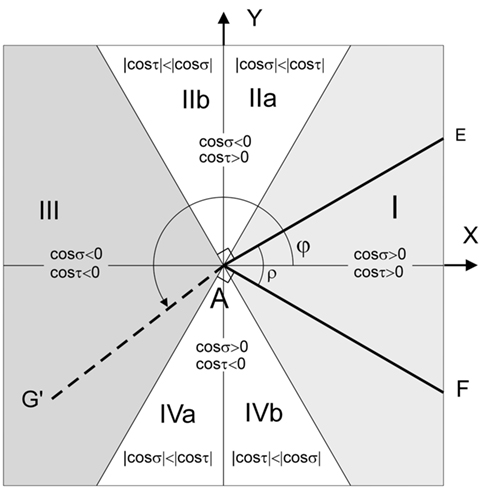
Figure A8. Areas of projection of parent segment G′A (I, IIa, IIb, III, IVa, and IVb, respectively) in the daughters’ plane to be distinguished for the transformation rules of the azimuth angle φ (see text). AE and AF are the daughter segments of a spatial bifurcation. ρ is the intermediate angle, and σ and τ are the side angles of the spatial bifurcations, see Figure 1B.
When projection in area I (see Figure A8), then cos σ > 0 and cos τ > 0.
Conditions for projection in area IIa (Figure A8) are cos σ < 0 and cos τ > 0 and |cos σ| < |cos τ|.
Conditions for area IIb are: cos σ < 0 and cos τ > 0 and |cos σ| > |cos τ|.
Conditions for area III are: cos σ < 0 and cos τ < 0.
Conditions for area IVa: cos σ > 0 and cos τ < 0 and |cos σ| < |cos τ|.
Conditions for area IVb: cos σ > 0 and cos τ < 0 and |cos σ| > |cos τ|.
This leads to the following transformation rules:
For projection onto area I, IIa, and IVb: φ = φ
For projection onto area IIb, III, and IVa: φ = φ + π
Finally, if φ < 0 then φ = φ + 2π
From (A28) and (A23) it follows, that

Expression of the parent elevation angle θ in terms of the bifurcation angles ρ, σ, and τ.
Extracting cos φ and sin φ from (A28) and (A29), respectively, and summing their squares yields

resulting in
With cos 2þeta = 2.cos2 þeta − 1 we obtain
and finally

and

Expression (A34) for the parent elevation angle θ is not symmetric in the bifurcation angles ρ, σ, and τ because of the choice of taking the spherical coordinates of the parent segments in a coordinate system aligned to the daughters’ plane and the daughters’ bisector. Eq. A34 is undefined when the intermediate angle ρ = 0, but then there is no bifurcation, or when ρ = π, in which case the bifurcation collapses into a plane of the parent segment and the oppositely aligned daughters, making þeta = 0°, and also the fold angle κ = 0°.
Dihedral Angle λ between the Planes Formed by the Parent and Each of the Daughter Segments
The dihedral angle λ measures the angle between the planes formed by the parent segment and each of the daughter segments (Figure A9). The dihedral angle λ can be expressed in terms of the bifurcation angles ρ, σ, and τ as follows:

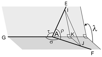
Figure A9. A spatial, non-recurrent bifurcation GAEF with dihedral angle λ between the planes formed by the parent segment AG and each of its daughter segments AE and AF, respectively. Intermediate angle ρ, and side angles σ and τ.
Thus
thus
and substituting the ratios by the sines and cosines we obtain

and thus
The dihedral angle λ is undefined when one of the side angles, σ or τ, equals zero, i.e., no bifurcation, or when one of the side angles is equal to 180°, but in that case the bifurcation is a side-branching bifurcation and thus planar and λ = 180°.
Dihedral Angle β between the Daughters’ Half-Plane and the Plane Determined by the Parent Segment and the Line Perpendicular to the Daughters’ Bisector at the Bifurcation Point.
The dihedral angle β is the angle between the daughters’ half-plane and the plane formed by the parent segment and the line perpendicular to daughters’ bisector through the bifurcation point A in the daughters’ plane (Y-axis; Figure A10). It can be expressed in terms of the parent elevation angle θ and azimuth angle φ of an aligned 3D bifurcation as follows.
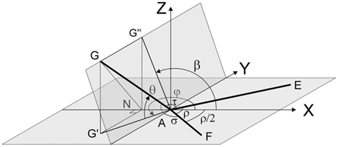
Figure A10. A spatial, non-recurrent bifurcation GAEF with the dihedral angle β, i.e., the angle between the daughters’ half-plane and the plane formed by the parent segment and the line in the daughters’ plane perpendicular to the bisector of the intermediate angle ρ, coinciding with the Y-axis due to alignment of daughters’ bisector with the positive X-axis. The azimuth angle φ is taken from the daughters’ bisector to the projection of the parent segment in the plane of the daughter segments.
We have GA = 1, G′G = sin θ, and G′A = cos θ, thus
Using (A32) we derive
When the parent segment is in the daughter plane (i.e., þeta = 0, thus tan þeta = 0), then β = 0 for cos φ > 0, and β = 180° for cos φ < 0. The dihedral angle β is undefined, when cos φ = 0 or when cos η = 0, in such a condition β = π/2.
Keywords: random spatial bifurcation, flatness measure, cone angle, solid angle right circular cone, solid angle triangular pyramid, dihedral angle, trihedral angle, symmetrical bifurcation
Citation: van Pelt J and Uylings HBM (2012) The flatness of bifurcations in 3D dendritic trees: an optimal design. Front. Comput. Neurosci. 5:54. doi: 10.3389/fncom.2011.00054
Received: 15 May 2011;
Accepted: 03 November 2011;
Published online: 25 January 2012.
Edited by:
Terrence J. Sejnowski, Salk Institute for Biological Studies, USAReviewed by:
Antonio Politi, Institute of Complex Systems, ItalyTatyana Sharpee, Salk Institute for Biological Studies, USA
Copyright: © 2012 van Pelt and Uylings. This is an open-access article distributed under the terms of the Creative Commons Attribution Non Commercial License, which permits non-commercial use, distribution, and reproduction in other forums, provided the original authors and source are credited.
*Correspondence: Jaap van Pelt, Computational Neuroscience Group, Department of Integrative Neurophysiology, Center for Neurogenomics and Cognitive Research, VU University Amsterdam, De Boelelaan 1085, 1081 HV Amsterdam, Netherlands. e-mail: jaap.van.pelt@cncr.vu.nl; Harry B. M. Uylings, Department of Anatomy and Neuroscience, VU University Medical Center, P.O. Box 7057, 1007 MB Amsterdam, Netherlands. e-mail: hbm.uylings@vumc.nl