1
Department of Psychology, University of Gießen, Giessen, Germany
2
Donders Institute for Brain, Cognition and Behaviour, Centre for Neuroscience, Section Neurophysiology and Neuroinformatics, Radboud University Nijmegen Medical Centre, Nijmegen, Netherlands
3
Center for Anatomy and Brain Research, University Clinics Düsseldorf, Heinrich Heine University, Dusseldorf, Germany
4
Department of Computer Science, Heinrich Heine University, Dusseldorf, Germany
In a recent paper (Reid et al., 2009
) we introduced a method to calculate optimal hierarchies in the visual network that utilizes continuous, rather than discrete, hierarchical levels, and permits a range of acceptable values rather than attempting to fit fixed hierarchical distances. There, to obtain a hierarchy, the sum of deviations from the constraints that define the hierarchy was minimized using linear optimization. In the short time since publication of that paper we noticed that many colleagues misinterpreted the meaning of the term “optimal hierarchy”. In particular, a majority of them were under the impression that there was perhaps only one optimal hierarchy, but a substantial difficulty in finding that one. However, there is not only more than one optimal hierarchy but also more than one option for defining optimality. Continuing the line of this work we look at additional options for optimizing the visual hierarchy: minimizing the number of violated constraints and minimizing the maximal size of a constraint violation using linear optimization and mixed integer programming. The implementation of both optimization criteria is explained in detail. In addition, using constraint sets based on the data from Felleman and Van Essen (1991)
, optimal hierarchies for the visual network are calculated for both optimization methods.
In 1991, Felleman and Van Essen formalized the idea of a visual cortical hierarchy using a large number of tract tracing results obtained from macaque monkeys. Their general premise was that the laminar source and termination patterns of corticocortical projections contained information about their hierarchical directionality, which allowed projections to be labelled as ascending, descending, or lateral. Using this information as a constraint, the authors presented a cortical hierarchy in which most of these direction relationships were satisfied (see Figure 4
, Felleman and Van Essen, 1991
).
Since the publication of this article, the question emerged: what is the optimal visual cortical hierarchy? Using the same set of criteria and notion of optimality, Hilgetag et al. (1996)
demonstrated that there are at least 100,000 hierarchies which are even more optimal than that introduced by Felleman and Van Essen (i.e., having less constraint violations). In Reid et al. (2009)
, we introduced a new approach to calculating hierarchies, which combined the laminar data from Felleman and Van Essen (1991)
with new concepts from Vezoli et al. (2004)
that permitted the additional representation of the hierarchical distance of a projection. Our approach utilized a continuous, rather than discrete scale for describing hierarchical level, and introduced the measurement of deviation from a constraint as a cost function for optimization, rather than a count of discrete violations. Although this method does not produce a unique optimal hierarchy – an indeterminacy problem similar to that reported by Hilgetag et al. (1996)
– it does always produce an optimal hierarchy. The method is also easily implemented, such that an optimal hierarchy can be calculated for any arbitrary set of cortical areas with tract tracing information, and easily updated if new data are produced.
A further question which emerges from this process is that of suitable optimization criteria. Whether a hierarchy is considered optimal depends on the notion of optimality that is employed, and there are many options for defining optimality. In Reid et al. (2009)
, we utilized the sum of deviations as an objective function to be minimized, but it is uncertain whether this is the best choice of criterion, and to what extent the addition of further objectives might improve the resulting hierarchy. This also introduces the related issue of how sensitive the optimization is to this choice of criteria. In the present article we explore these possibilities, investigating in particular the effects of adding (1) the number of violations, and (2) the maximal deviation, to the objective function.
Graph Representation and the Hierarchy Function
Consider a network representing a hierarchy given as a directed graph G = (V, E), where V is a set of vertices and E a set of directed edges. Each edge in the graph is assigned a weight that signifies the possible range of distances of its endpoints within the hierarchy (see Figure 1
for an example).
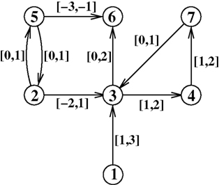
Figure 1. A directed graph with vertices v1,v2,v3,v4,v5,v6,v7 and edge ranges.
If the edge runs from vertex u to vertex v then an interval [x, y], x, y ∈ ℝ is assigned to that edge and the hierarchical distance between u and v should lie within this interval (see Figure 2
). A positive distance value implies the edge is going up and v is above u in the hierarchy. A negative value means that the edge is descending with regard to the hierarchy and v is below u in the hierarchy. The value 0 signifies that the edge does not cross levels in the hierarchy and u and v are on the same level.
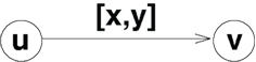
Figure 2. Vertices u and v with the hierarchical distance [x,y].
To find the hierarchy implied by these edge values we are looking for a function h: V → ℝ so that for every edge (u, v) with assigned interval [x, y], x, y ∈ℝ the following conditions hold:

This function h is called the hierarchy function.
However for the example in Figure 1
it is not possible to find such hierarchy functions because the distance information is not consistent. The alternative is to find a hierarchy function that “best” fits the data. To do so it is necessary to allow some deviations from the given data. To measure this deviation we introduce a variable Δ(u,v) for every edge (u, v). A variable Δ(u,v) measures for the two conditions defined by the edge (u, v) how much the hierarchy violates these conditions. This alters the condition for the hierarchy function resulting from an edge (u, v) with a range [x, y] in the following way (compare Figure 2 and Eq. 1):

With these inequalities we allow a deviation of Δ(u,v) from the constraints assigned to an edge (u, v) by the interval [x, y]. The Δ(u,v) is specific for every edge (u, v) which means one distinct variable Δ(u,v) for every edge is needed. Ideally, the value of these Δ(u,v) should be kept as small as possible, preferable 0. Since all Δ(u,v) measure a deviation, their values are always non-negative. Also note that at most one of the two conditions for an edge (u,v) can require an Δ(u,v) larger than 0. The objective is now to find a hierarchy that best fits the data, i.e., with as little overall deviation as possible. To accomplish this the sum of all deviations Δ(u,v) should be minimal.
To calculate such an hierarchy we use a well known method called linear programming. A detailed introduction on linear programming can be found (for example) in the book of Papadimitiou and Steiglitz (1998)
. In brief the aim of linear programming is the optimization of a linear objective function, subject to linear equality and inequality constraints. Those linear problems have the following form, which is also called linear program:
Maximize/minimize the expression

subject to constraints
Here x1,x2,…,xn are variables, for which values need to be found. All other elements are constants.
There are different ways to solve these kinds of problems. The oldest and most widely used is the simplex algorithm which was developed in 1947 by Dantzig (see for example Dantzig, 1963
). It has an exponential worst case run time but most instances can be solved much faster. Today the inner point method invented by Karmarkar (1984)
is often used as well, which has a polynomial runtime. For this work the optimization procedure was performed using the Gnu Linear Problem Kit
1
which can be used for linear programming as well as mixed integer programming.
Example
Consider the example in Figure 1
. We are looking for a hierarchy function h: V → ℝ with h (v1) = 0 and for all (u, v) ∈E with edge value [x, y] the conditions h(u) + y + Δ(u,v) ≥ h (v) and h (u) + x − Δ(u,v) ≤ h (v) should hold (compare to Eq. 2).
From these inequalities we receive the following two conditions for every edge:

Since we want to calculate the values of the hierarchy function h for every v ∈V we also include h(v) as a variable in the linear program. To make the notation easier these variables will receive the names of the vertices in the linear program. So for every v ∈V there is a variable v that represents the function value h(v) in the program.
With this replacement the conditions in the program look like this

With those inequalities we can create a linear program to calculate an optimal hierarchy for the example in Figure 1
. The objective of the program is to minimize the sum of all deviations. (see Figure 3
, left: the variable sumΔ is the sum of all deviations.)
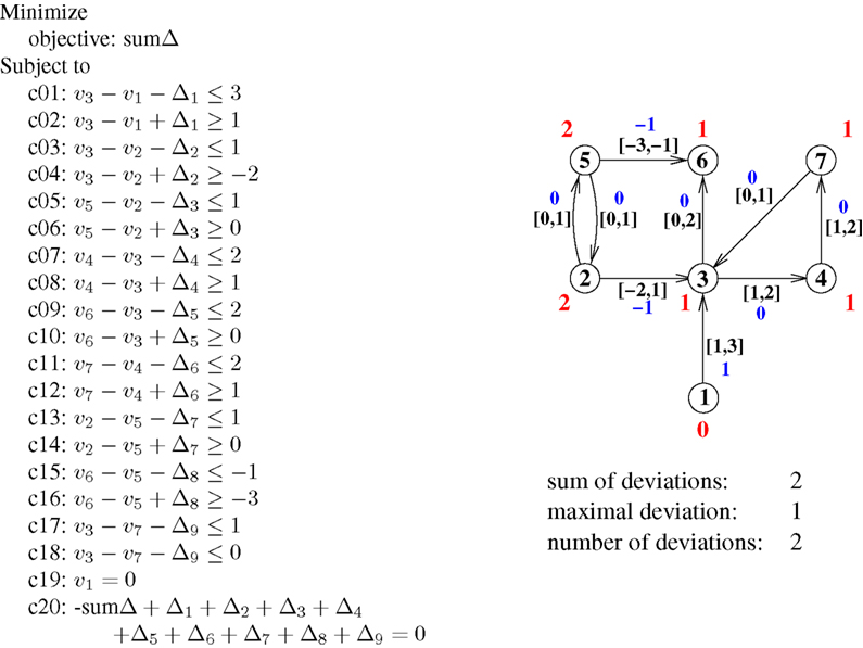
Figure 3. Left: The linear program to calculate an optimal hierarchy for the graph from Figure 1
. The objective is to minimize the sum of all deviations (defined by constraint c20). Right: The resulting hierarchy. Red numbers are the hierarchy levels of nodes, blue numbers the actual distances in the hierarchy.
The node v1 is supposed to be the starting point of the hierarchy, and therefore its value is fixed at 0. The variables v1 to v7 are not limited by the optimization objective (c20), and thus can become as big or small as necessary to attain the optimal value for sumΔ.
Additional Objectives
So far our objective for finding an optimal hierarchy is to keep the sum of deviations as small as possible for the given edge values. But since there is normally more than one hierarchy that fulfils this objective, it can be useful to employ additional secondary objectives. We will illustrate this by an example.
Consider graph A of Figure 4
. Since the sum of all edge values in that circle is 1 the minimal sum of deviations of any hierarchy for this graph is 1. The question is how that sum is best distributed on the involved edges. One option is to concentrate the deviation on as few edges as possible. That does not change the sum of deviations but it keeps the number of violated conditions small (see Figure 4
B). Another possibility can be seen in Figure 4
C, there the deviation is distributed on all edges. This keeps the maximum deviation small and therefore all distances imposed by the hierarchy close to the original edge weights. Figures 4
B,C are not the only options for an optimal hierarchy. Note that there is an infinite number of other hierarchies with a minimal sum of deviations for this example.
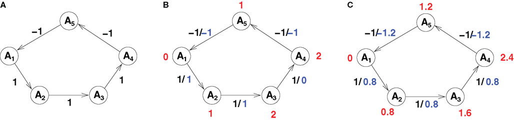
Figure 4. (A) A graph with edge values. (B) One possible hierarchy obtained by optimizing for the number of constraint violations. (C) Another possible hierarchy obtained by optimizing for the maximum deviation. Both (B) and (C) red numbers are the hierarchy levels of nodes, blue numbers the actual distances in the hierarchy.
The question is: which hierarchy describes the information given by the edge values best? The advantage of minimizing the number of violations is that most of the original distance information is preserved in the hierarchy, and we ideally disregard only the information that fits the model the least. Minimizing the maximum deviation, alternatively, has the advantage that all the information is treated equally and non is disregarded completely. The rationale for this is that it is better to change many distances a little than few distances a lot.
To implement these additional objectives, additional variables are needed in the program. In the first case it is necessary to count and minimize the number of violations, which can not be done with just linear programming, but rather requires the use of mixed integer programming. For the second option we need to minimize the maximal deviation, which can easily be integrated in the linear program, so it will be discussed first.
Maximal deviation
To calculate the maximal deviation of the hierarchy we introduce a variable Δmax which measures the maximal deviation from any constraints. To implement this every constraint of the original program is doubled and in the second version the specific Δ(u,v) for the edge is replaced by the global Δmax. So we now have four conditions in the program for an edge (u,v) with edge value [x,y] (compare Eq. 5):
If one of the original constraints only holds if Δ(u,v) is greater than 0, then Δmax needs to be as least as big as Δ(u,v) for the doubled constraints to hold as well. Since this is true for every constraint it means Δmax needs to be at least as large as the largest edge specific deviation. If Δmax is included in the objective to be minimized it will take exactly the value of the maximal edge specific deviation Δ(u,v).
Since the prime objective is still to minimize the sum of all deviations we introduce a factor in the objective to give the sum of deviations a bigger weight than the maximal deviation Δmax. The factor needs to be large enough that the smallest edge-specific deviation Δ(u,v) multiplied by the factor is considerably larger than Δmax. This ensures that Δmax is not of the same magnitude as the sum of deviations with regard to the optimization and therefore does not influence the primary optimization goal. The result is a hierarchy with a minimal sum of deviations, but among those hierarchies one with the smallest possible Δmax is chosen.
As factor we used 100 which proved to be large enough that the resulting hierarchy is still one with a minimal sum of deviations, so it fulfilled the requirements outlined in the previous paragraph. The results for the graph from Figure 1
are shown in Figure 5
A (compare to Figure 3
).
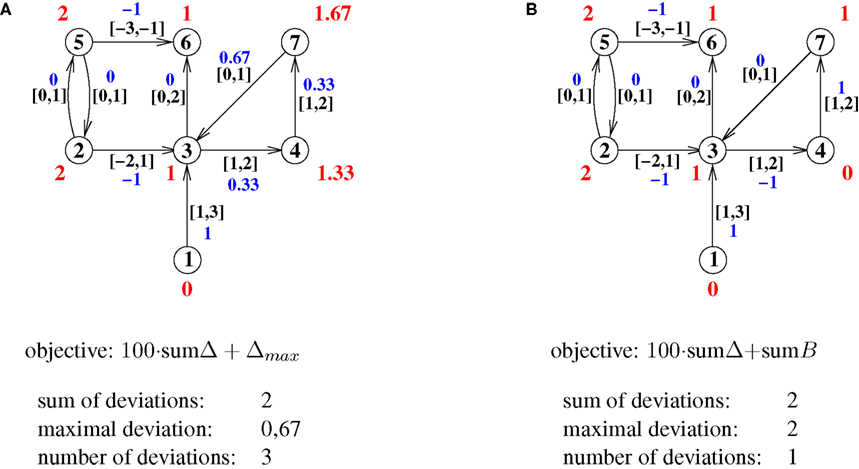
Figure 5. (A) An optimal hierarchy for the graph from Figure 1
given the objective to minimize primarily the sum of all deviations and in addition the maximal deviation. Red numbers are the hierarchy levels of nodes, blue numbers the actual distances in the hierarchy. (B) An optimal hierarchy for the graph from Figure 1
given the objective is to minimize primarily the sum of all deviations and in addition the number of deviations. Again, red numbers are the hierarchy levels of nodes, blue numbers the actual distances in the hierarchy.
Number of violations
To minimize the number of violations in a hierarchy it is necessary to count them within the program. To accomplish this we introduce an edge-specific integer variable B(u,v) which assumes the value 1 if Δ(u,v) > 0 and 0 if Δ(u,v) = 0. The sum of these violation counters can then be included in the objective to be minimized along with the sum of the deviations. These variables are not reals but integers, so it is necessary to use mixed integer programming. Mixed integer problems look like the linear problems we have seen so far (compare again to Eq. 3), but some of the variables can only take integer values. This gives the optimization problem a higher complexity: other than linear optimization problems, mixed integer problems can in general not be solved efficiently, they are NP-hard. While there are well-known algorithms to solve these problems, one of the first was developed by Land and Doig (1960)
, this does not mean that solutions can actually be found for all mixed integer problems as there are limitations of computer memory and time.
A problem with the implementation is that an integer variables B(u,v) could take any non-negative integer value, but we want them to only take the values 0 and 1. To ensure this we use a trick: For the program we double every constraint from the original program and get four conditions for an edge (u,v) with edge value [x,y] (compare Eqs 5 and 6):
The two original conditions measure once again the size of a deviation from a constraint and the two new conditions test if there actually is a deviation. The factor 100 in front of the B(u,v) is much bigger than any number that actually occurs in the calculation. If we look at one of the conditions from Eq. 7, say v − u − 100·B(u,v) ≤ y then if v − u ≤ y the variable B(u,v) can assume the value 0. If on the other hand v − u > y then the variable B(u,v) needs to be at least 1 for the second inequality in Eq. 7 to hold. (Remember, unlike Δ(u,v) the variable B(u,v) is an integer and does not take values between 0 and 1.) Since the factor 100 is chosen to be a lot bigger than |v − u − y| the inequality v − u − y − 100·1 ≤ 0 always holds. Therefore, with B(u,v) = 1 the constraint is fulfilled, and there is no need for any B(u,v) to be bigger than 1. By the same argument as above for Δmax we get

if the sum of all B(u,v) is included in the objective to be minimized. The results for the graph from Figure 1
is shown in Figure 5
B (compare to Figure 3
).
Note that all three examples have the same sum of all deviations since it is primarily being optimized in all three cases. The differences lie in the second part of the objective, i.e. the maximal deviation and the number of deviations. Also note that the hierarchies shown here are again not the only optimal hierarchies that can be found for these criteria.
Empirical Data
We use the data set described by Felleman and Van Essen (1991)
for the visual system of the macaque monkey (FV91). As regions MDP and MIP had no constraints defined, they are not included here. The projections in this network were assigned ranges according to a modification of the original relationship classification scheme, which incorporates ideas presented in subsequent publications (Kennedy and Bullier, 1985
; Barone et al., 2000
; Batardiere et al., 2002
), and permits a richer representation of hierarchical distance and the assignment of refined ranges (compare to Reid et al., 2009
). As in Reid et al. (2009)
we use the notation A+ for strongly ascending, A for ascending, L for lateral, D for descending and D+ for strongly descending projections. To investigate the effect of range sizes upon the resulting optimal hierarchies, ranges were varied from disjoint intervals with clear gaps between the five connection types to intervals that overlap so that the connection types are merging into one another. To implement this ranges were systematically expanded by 0.1 at each limit, resulting in 10 range sets, as presented in Table 1
. The outer bounds for these hierarchies were chosen as 32, which is the total number of regions; this ensures that no individual projection can have a hierarchical distance greater than the total number of regions.
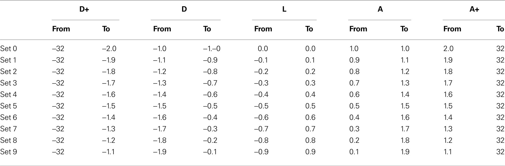
Table 1. The borders of the ranges for the different constraint sets.
We employed two different optimization methods: For the first we minimized the objective 1,000·sumΔ(u,v) + sumB(u,v). For the second we minimized the objective 1,000,000·sumΔ(u,v) + 1,000Δmax + sumB(u,v).
The two optimization methods produced similar, but not identical results. Table 2
shows the values for the sum of deviations, the maximal deviation and the number of violations for the optimal hierarchies. For comparison the values from Reid et al. (2009)
are also included. There only the sum of deviations was minimized and the optimization was performed using the QS-Opt Linear Problem Solver
2
. Note that the sum of deviations is the same for each set for all optimizations, since this was always the first objective.
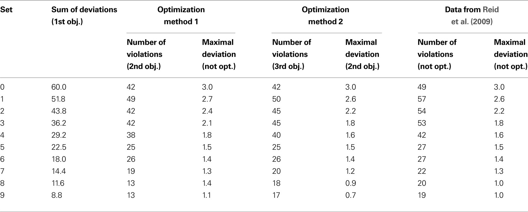
Table 2. The results of the optimization.
With the exception of number of violations for set 0 the optimized values are getting smaller when the size of the constraining intervals is getting bigger. The sum of deviations goes down from 60.0 for set 0 to 8.8 for set 9, the maximal deviation is reduced from 3.0 for set 0 to 0.7 for set 9 with optimization method 2, the number of violations decreases from 49 for set 1 to 13 for set 9 with optimization method 1 and from 50 for set 1 to 17 for set 9 with optimization method 2.
For three sets (0, 5 and 6) we get exactly the same optimal values for both optimization methods, but only for one of these sets (set 0) are the calculated hierarchies identical. For set 5 and set 6 the two calculated hierarchies are not identical. However, for each set both hierarchies have the same number of violations and maximal deviations, which means that they are both optimal hierarchies for both optimization methods. The corresponding hierarchies from Reid et al. (2009)
all have the same maximal deviation but larger numbers of violations, so regarding the number of violations these hierarchies are not optimal. In general the number of violations for the hierarchies from Reid et al. (2009)
are higher than for the new optimization methods, but since the violations were not minimized before this is not surprising. However the maximal deviations tend to be small, often minimal (as seen in comparison with optimization methods 2), for these hierarchies, even though they were not minimized.
For all other sets than 0, 5 and 6, we see differences in values between the two new optimization methods, therefore there is a trade-off between the number of violations and the maximal deviations. Therefore these values cannot both be at their minimum for 7 of the 10 sets.
When we look at the violated constraints we find only a total number of 54 of the 386 constraints being violated by either of the two optimization methods. Of those nine constraints were violated by every set for both methods (see Table 3
). Note that everything is counted as a constraint violation that does not exactly fit the classification of a connection. For example, if a connection is classified as ascending (A) but ends up being strongly ascending (A+) in the calculated hierarchy this counts as a violation. Also note that for all the connections listed in Table 3
there are reciprocal connections that were not consistently violated. This means that the classification of these reciprocal connections is not complementary. For example the connection V2 to V3 is classified A+, but the connection V3 to V2 is classified D (not D+).
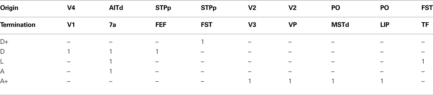
Table 3. The 9 constraints that are violated by all 10 sets for both objectives. The number 1 means the corresponding connection is classifi ed as D+, D, L, A or A+.
The two optimization methods generally violated the same constraints: For the first optimization method 53 and for the second optimization method 52 different constraints (of 386) were violated over the 10 sets and of those 51 constraints were violated by both methods. In addition constraint V1 to V3 (A+), was violated by the second optimization in four sets and constraints LIP to V4 (D), and 46 to TH (L), were each violated by the first optimization in one set.
For comparison between sets we normalized the resulting hierarchies: by definition V1 always had the hierarchical value 0, the region with the highest hierarchical level was assigned the value 1, the hierarchical levels of the other areas were transformed accordingly. Figure 6
shows the average hierarchical levels over the 10 sets for the first optimization method. The equivalent figure for the second optimization method looks very similar and is therefore not included here.
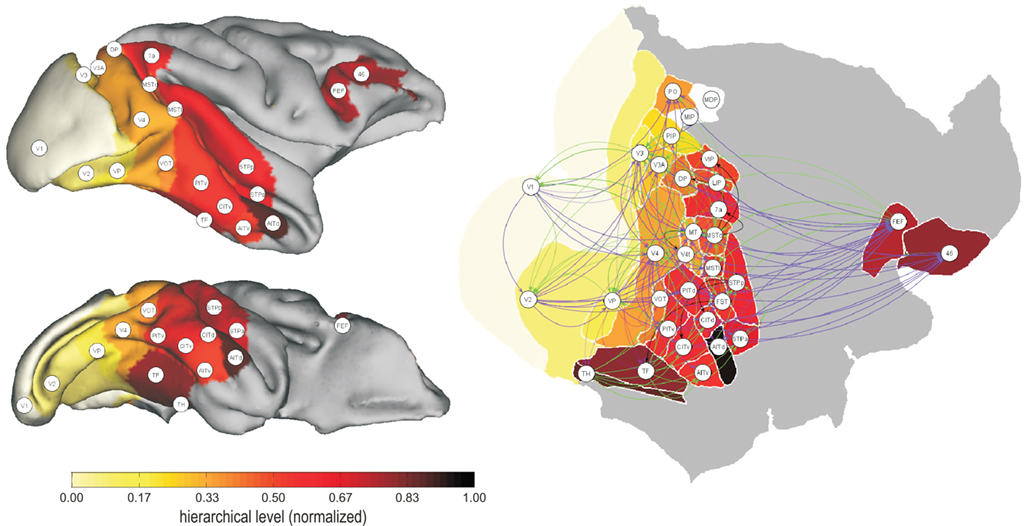
Figure 6. Geometrical distribution of hierarchy levels in the FV91 visual network of the macaque, both as three-dimensional cortical surface renderings (left), and as a two-dimensional “flat map” representation of the cortical sheet (right). Regions are coloured by their mean normalized hierarchical position, obtained by the first optimization method over the 10 constraint sets described in Table 1
. Directed edges in the flat map illustration represent interregional connections, and are coloured according to projection class: A+ (purple, opaque), A (purple, transparent), L (black), D (green, transparent), and D+ (green, opaque). Compare this representation to Figures 2 and 4 in Felleman and Van Essen (1991)
.
While the parameters for the hierarchies do show some differences between the optimization methods, the resulting hierarchies were remarkably similar. This does not mean that all hierarchies that are optimal for the two optimizations are similar: since we only have one possible solution per optimization method per set there might also be solutions that differ substantially. What it does mean is that there are examples for optimal hierarchies for the two optimization methods for which the differences between the optimized values seem to be accomplished through minor changes within the hierarchies.
The boundaries chosen for the optimization constraints (set 0 to 9) seem to have a big influence on the optimization results. All optimized values for set 0 are several times as big as the corresponding values for set 9. The “looser” the boundaries are (i.e., the larger the defining intervals) the smaller the optimized values. This is because in the bigger intervals for the connection classes more values can be assumed in the optimization without violating the constrains. For example, if an ascending connection is assigned the value 1.5, this is a violation in sets 0 through 4, but not in sets 5 through 9. Therefore there are fewer violations and, as a result, smaller optimized values for sets that use bigger intervals for connection classes. However in Reid et al. (2009)
we found that the resulting hierarchies are very comparable across sets after normalization. There were only minimal changes in the order of the areas in the calculated hierarchies for the different conditions.
The similarity in the violated constraints across methods suggest that these constraints may be erroneous. In particular, of the nine constraints that are violated in this study by all constraint sets, and for both objectives, eight were violated in the calculations of Reid et al. (2009)
for all constraint sets as well. [The last of the nine constraints, PO to LIP (A+), was violated by eight sets in Reid et al. (2009)
. While it is possible that a solution exists where none of these constraints are violated, this consistency suggests a pattern which is worth further investigation. The fact that all of these connections have reciprocal connections whose constraints are not consistently violated seems to suggest that the classification of the reciprocal connections fits an optimal hierarchy better than the classification of the nine violated connections. Since the classification of the reciprocal connections is not complementary at most one of the classifications (the one for the connection or the one for the reciprocal connection) can be correct. This does not necessarily mean that the classification is better for the reciprocal connection since in some cases this classification is very broad, spanning several of our five classes.
The classical optimization problem of minimizing the number of violations [as done by Felleman and Van Essen (1991)
as well as Hilgetag et al. (1996)
can theoretically be solved by the method presented here, where it was only used as an secondary objective. In practical terms, solving for number of violations as a primary objective has proven too computationally expensive, whereas using it only as a secondary objective made the calculation easier, since the solutions were already limited by the minimal sum of deviations. However, we were able to minimize just the number of violations for sets 8 and 9, which produced the smallest optimal values for all the other optimization methods. The results (12 violated constraints with a sum of deviation of 13.4 for set 8, and 11 violated constraints with a sum of deviations of 10.7 for set 9) are only slightly below the number of violated constraints for optimization method 1.
The hierarchies calculated here are of course also solutions for the original optimization problem from Reid et al. (2009)
, since they have the same minimal sum of deviations. Additionally, however, they also have either a minimal number of violations or a minimal maximum deviation, and in some cases even both. This added optimality does not seem to be especially advantageous, however, given that the resulting hierarchies remained for the most part unchanged, which suggests that they are not highly sensitive to the addition of these criteria. Other objectives are also conceivable, of course, which may result in more strongly altered hierarchies than we report here. For instance, it is conceivable that further knowledge about the reliability of the anatomical data underlying our constraints may yield more informative objective criteria, that would allow a Bayesian approach to this problem. Another option is not to allow any deviation for connections that are classified with a great certainty, ensuring that the connection appears as classified in the hierarchy. However, this cannot be done for all connections since the resulting constraints are not consistent and some deviation needs to be allowed to find an hierarchy.
In the choice of the optimization method the data quality should be considered. If we expect that most of the connections are correctly classified but there might be some classifications that are erroneous then minimizing the number of violations is the better option. Most of the distance information of the classification should then be preserved in the hierarchy. Assuming that the wrongly classified connections are the ones that do not fit the hierarchy these would be the ones that are disregarded. They would be “taken out” of the hierarchy. If on the other hand, we expect all the classifications to be equally correct or faulty (or just an approximation of the true value), then we want to consider all the information to the same degree. This can imply changing many classifications a little to “squeeze” the information into a hierarchy, such that, ideally, none of the information is disregarded completely, while many of the classifications might be “corrected” a little.
Since our results produced highly similar hierarchies across a variety of constraint sets for the two optimization methods presented here, both appear equally suited for the calculation of optimal hierarchies. It is thus a matter of personal preferences which one to employ, and this choice is one that can conceivably be expanded to accommodate alternative definitions of optimality. This leads us to conclude that there is no unique optimal hierarchy, not only because of the quality of the empirical data and the freedom to choose boundaries for the defining intervals, but also because there is more than one way to define optimality. While the method described does not provide a unique optimal hierarchy, it can produce hierarchies that are optimal in more than one way.
The authors declare that the research was conducted in the absence of any commercial or financial relationships that could be construed as a potential conflict of interest.
Rolf Kotter and Egon Wanke received funding from the DFG (KO 1560/6-2, WA 674/10-2). Andrew T. Reid, Gleb Bezgin and Rolf Kotter were funded by a collaborative network grant from the McDonnell Foundation. The authors acknowledge funding received by the Initiative and Networking Fund of the Helmholtz Association within the Helmholtz Alliance on Systems Biology.