Wanted dead or alive? The tradeoff between in-vivo versus ex-vivo MR brain imaging in the mouse

1. Introduction

Imaging is a key tool for tracking changes in the anatomy of the brain across time. In human studies, the aim is to assess alterations that have occurred over periods ranging from hours to years and test whether these differ by diagnosis, treatment group, or outcome.

Tracking changes in neuroanatomy over time has been essential for neurodegenerative diseases. Hippocampal atrophy in Alzheimer's disease (Chetelat, 2003; Silbert et al., 2003; Zakzanis et al., 2003) or striatal atrophy in Huntington's (Montoya et al., 2006; Paulsen et al., 2006) are respective hallmarks of disease progression or even prodromal indicators of likely future diagnosis (Paulsen et al., 2008). Similarly, alterations in atrophic progression are potential biomarkers of treatment efficacy. Stopping or slowing hippocampal or striatal atrophy may represent early indicators of successful therapy. In addition to the disease or treatment examples, changes in anatomy over time are increasingly being used as an indicator of neuroplasticity. Naive subjects learning to juggle (Draganski et al., 2004; Boyke et al., 2008; Driemeyer et al., 2008; Scholz et al., 2009) or play musical instruments (Gaser and Schlaug, 2003; Hyde et al., 2009) are just two examples where short term changes in gray and white matter have been detected.

To understand the mechanisms of this anatomical change in the brain over time, it has become increasingly beneficial to study the mouse, wherein observation of anatomical changes can be coupled with both precise control of genetic and environmental factors and with detailed measurements (histology and immunohistochemistry). This allows one to determine what causes the brain to change and how it does so. In the case of brain plasticity, for example, we have shown that 5 days of training mice on a maze is sufficient to cause MR-detectable hippocampal and striatal volume changes on the order of 2–4% that correlate with expression of a marker of neuronal process remodeling (Lerch et al., 2011). Similarly, multiple groups have been able to use MR imaging of mouse models of Alzheimer's or Huntington's to monitor progression of atrophy and relate these volumetric changes to other biochemical markers (Lau et al., 2008; Lerch et al., 2008; Badea et al., 2010; Sawiak et al., 2009; Carroll et al., 2011).

MR imaging of the mouse involves tradeoffs due to the size of the animal. To gain comparable information to the common human anatomical imaging studies, voxel sizes on the order of tens of microns to a hundred microns are required. Obtaining such resolution is accomplished through higher field strengths, custom-designed coils, optional use of contrast agents and significantly longer scan times. The duration of in vivo imaging sessions is, however, limited by the approximately 3 h anesthesia tolerance of mice, resulting in isotropic voxel sizes of around 100 μm. Another option is ex-vivo fixed-brain imaging, where the combination of much longer scan times, tighter fitting radiofrequency coils, and high-dose gadolinium-based contrast agents allows for improved image resolution and contrast.

There is, therefore, also a natural tradeoff between in-vivo and ex-vivo imaging, with longitudinal capabilities in the case of the former but the possibility of higher resolution and sensitivity in the case of the latter. Naturally, the greatest phenotype detection sensitivity will always be achieved by performing as many high-resolution fixed specimen scans as is feasible at the single timepoint when anatomical change is the greatest. Rarely in academic research is there enough prior information available to permit the design of a study of this kind. Rather more frequently, one is interested in characterizing a process of change that has only a vaguely defined timecourse and that may affect multiple—probably as yet unidentified—structures. In this case, there is a need for both temporal and spatial sensitivity and the tradeoff between the two is entangled with the tradeoff in performance between in-vivo and ex-vivo mouse imaging.

The goal of this manuscript is to provide a statistical exploration of the tradeoffs between in-vivo and ex-vivo mouse imaging in this context. For the sake of simplicity, and to provide a concrete example, we focused the statistical study on a hypothetical experiment in which we seek to recover a 3% change in the volume of the hippocampus. First, we characterize the relative contributions of different sources of variance to our estimate of hippocampal volumes. Second, we use these measures to simulate a timecourse experiment and determine phenotype detection sensitivity while changing the number of subjects, the number of time points and the measurement variance. Finally, we consider the characterization of rate of change over time with both a longitudinal, in-vivo imaging experiment and a purely cross-sectional, ex-vivo experiment. We expect that this analysis will provide guidelines helpful in planning mouse imaging experiments and provide rules of thumb for selection of in-vivo vs. ex-vivo study designs.

2. Methods

We explore the trade-offs involved in designing mouse imaging experiments by first estimating variance in hippocampal volumes in:

• eight 12-week-old C57Bl/6 mice imaged using a high-resolution fixed-brain sequence to estimate population variability in volume;
• the same mice imaged using a lower-resolution sequence to estimate the effects of resolution on variance;
• each of the above two studies repeated three times on the same specimens to measure pure imaging and algorithmic noise; and
• eight mice imaged in-vivo at 24, 42, and 63 days of age to estimate variability in repeatedly imaging the same animal.

2.1. Data acquisition

2.1.1. Ex-vivo high-resolution

Animals were prepared for ex-vivo imaging by perfusion fixation. For this purpose, animals were deeply anesthetized with a ketamine-xylazine mixture (150 mg/kg and 10 mg/kg, respectively) and then intracardially perfused first with phosphate-buffered saline (PBS), heparin and 2 mM ProHance (gadoteridol, Bracco Diagnostics Inc., Princeton, NJ) and second with 4% paraformaldehyde (PFA) and 2 mM ProHance. After perfusion, all extracranial tissue was removed and brains were left in the skulls and soaked in 4% PFA with 2 mM ProHance for 12 h and then in PBS with 2 mM ProHance for at least 1 week. A multi-channel 7.0 T, 40 cm diameter bore magnet (Varian Inc., Palo Alto, CA) was used to acquire all images for this study. High-resolution, ex-vivo scans were acquired using a T2-weighted, fast spin-echo sequence with parameters: 2 s repetition time (TR), 42 ms effective echo time (TE), 6 echoes at 14 ms echo spacing, 25 × 14 × 14 mm field-of-view (FOV), 450 × 252 × 250 matrix, and twofold oversampling in the first phase encode dimension (equivalent to acquiring two averages) for a total scan time of 11 h 40 mins.

2.1.2. Ex-vivo low-resolution

Low-resolution, ex-vivo scans of the same samples were acquired using a T2-weighted, fast spin-echo sequence with parameters: 0.95 s TR, 42 ms effective TE, 6 echoes at 14 ms echo spacing, 25.1 × 14.5 × 14.5 mm FOV, 228 × 132 × 132 matrix, and twofold oversampling in the first phase encode dimension (equivalent to acquiring two averages) for a total scan time of 1 h 32 mins.

2.1.3. In-vivo longitudinal

In-vivo images were acquired in mice with manganese (Mn) enhanced MRI. For this purpose we made a 300mM stock solution from manganese (II) chloride tetrahydrate from Sigma-Aldrich in cell culture grade water from Fisher Scientific. This was then diluted 10× with 0.9% sodium chloride to 30mM for intraperitoneal injection into the mice (0.4 m mol/kg dose). Twenty-four hours following Mn-injection, mice were anesthetized for imaging with 4% isoflurane and then placed within the magnet bore for imaging. Mice were maintained on 1% isoflurane at a body temperature of 35°C according to established protocols. In-vivo, Mn-enhanced images were acquired using a spoiled gradient-echo sequence with parameters: 0.1 s TR, 3.7 ms TE, 55° flip angle, 280 × 168 × 168 matrix, 35 × 21 × 21 mm FOV, with two averages for a total scan time of 1 h 34 mins.

All animal experiments were performed in accordance with protocols approved by the Toronto Centre for Phenogenomics Animal Care Committee.

2.2. Data Processing

Data processing was performed separately for each of the data-sets described above and is explained in detail in (Lerch et al., 2011). Briefly, all scans were aligned toward a consensus average using a three step process. An initial rigid-body alignment was used to orient all brains in the same coordinate space. Pair-wise 12-parameter linear alignment is then employed to create an unbiased linear average of all brains in each experiment. Lastly, iterative deformable registration then creates a final average with any remaining local differences between brains removed. A combination of ANIMAL (Collins et al., 1994, 1995) and ANTS (Avants et al., 2008) was used to compute the registrations. A previously created segmented atlas (Dorr et al., 2008) was then deformed toward each data-set's population average and the volume for each scan's hippocampus extracted. When compared to manual segmentation this automated procedure achieves a Kappa of 0.86 (with a range of 0.85–0.88), which is high (Chakravarty et al., submitted). Based on these data, we computed mean and standard deviations of hippocampal volume measurements for each scan type. Using the repeated scan measurements, we were able to estimate both a population standard deviation (which includes biological and measurement noise) and a within-subject standard deviation (which includes only measurement noise when scanning the same subject). These noise source estimates were subsequently used in our statistical simulations.

2.3. Statistical Simulations

The key terms in our statistical simulations are shown in Table 1. The data at each timepoint is simulated in the following way:

TABLE 1

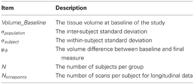
Table 1. The key parameters in simulating change over a short period of time.

We assume a linear change with equally spaced timepoints. For the following studies we have set μ_β to be 3%. Each of the following experiments will draw 1000 samples per quantity to be estimated to study the effects of varying subjects per group, scans/timepoints per subject, and the two sources of noise (σ_population and σ_subject). An example simulated dataset based on those numbers is shown in Figure 1. All simulations were carried out in R statistical environment (www.r-project.org) using the rnorm function for drawing random numbers from the normal distribution.

FIGURE 1

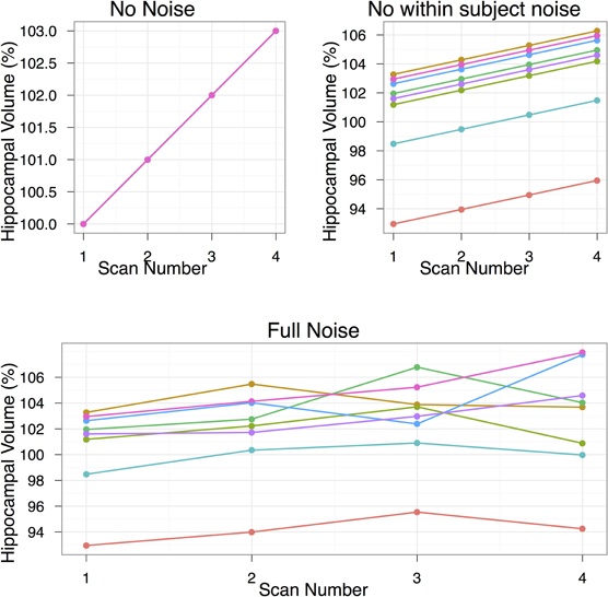
Figure 1. The data simulation, shown under three conditions of no noise, only population noise, and both population and subject noise. The population noise is representative of biological variability. Subject noise includes a combination of factors including imaging method and registration algorithm noise that affects the ability to produce the same result on repeated scans. In all cases we start with hippocampal volume at 100%, and by the end of the study that volume is to increase by 3%. The second group, not shown, is a control group with no hippocampal volume changes. The simulation shown in this figure includes eight subjects per group and four scans per subject.

3. Results

3.1. Contributions to the Variance of Hippocampal Volume Measurements

To estimate the variance contributions to hippocampal volume measurements, we imaged mice repeatedly at high-resolution ex-vivo, at low-resolution ex-vivo and longitudinally in-vivo. Sample images are provided in Figure 2. After registration of all images to an unbiased, consensus average, the volumes of the hippocampus and whole brain were extracted. As can be seen in Table 2 the population standard deviation in hippocampal volume ranges between 4.8% and 5.0%, depending on the scan type. Hippocampal volume estimated from scanning the same fixed-brain specimen repeatedly, however, showed a standard deviation of only 1.1–1.3%, depending on the image resolution. The implication is that the majority of variance in our imaging measurements is biological, not methodological. Moreover, we observed that a significant proportion of the variance in hippocampal volume is accounted for by overall differences in brain volume. This is made clear by considering hippocampal volumes normalized by brain volumes (Table 2), which have standard deviations reduced to 1.7–3.0% for the population and to 1.0% for repeat scans. A scatterplot of hippocampal volume to brain volume is provided in Figure 3 and shows the two volumes are highly correlated.

FIGURE 2

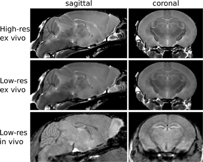
Figure 2. Sample images from the three acquisitions used in this study are shown here.

TABLE 2

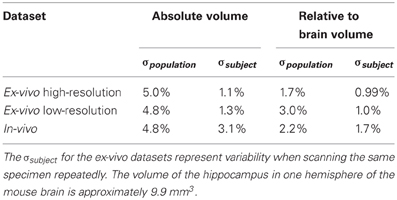
Table 2. Standard deviations (expressed as percent of hippocampal volume) across three datasets.

FIGURE 3

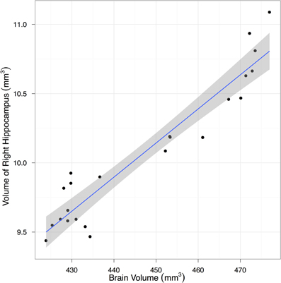
Figure 3. A scatter plot showing the correlation between hippocampal and total brain volume from fixed-brain specimens. Regression line and its 95% confidence interval are superimposed.

3.2. Factors Affecting the Detection of Anatomical Phenotypes in in-vivo Timecourse Experiments

We next performed a series of simulations to determine possible outcomes in a timecourse experiment in which we supposed a 3% change in the volume of the hippocampus. We independently varied the number of uniformly spaced timepoints per subject, the within-subject standard deviation (i.e., the measurement error associated with each scan), and the number of animals in each of two groups (an affected group vs. a control group with no change). In these cases, and based on the variance measurements from our in-vivo imaging data, the key to recapturing the simulated change is to ensure at least one of the following conditions is satisfied:

1. the number of timepoints per subject is at least six (with 10 subjects per group and a 3.1% standard deviation, Figure 4);
2. the imaging method is improved to reduce the within-subject standard deviation (i.e., the standard deviation associated with repeated scans of the same mouse) to less than 2.7% (with 10 subjects per group and four imaging timepoints, Figure 5); or
3. there are 12 or more animals per group (with four imaging timepoints and 3.1% standard deviation, Figure 6).

FIGURE 4

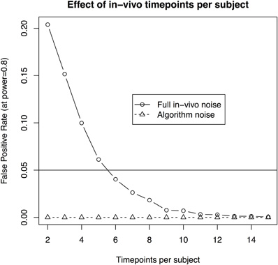
Figure 4. The effect of scans per subject when assuming 10 subjects per group and aiming to recapture a 3% change in volume in a longitudinal in-vivo study. The solid line illustrates the statistical power using a standard deviation of 3.1%, as estimated from the in-vivo data. The dotted line shows the estimate based on a reduced standard deviation of 1.1%, the best estimate obtained by repeated scans of ex-vivo samples. The latter gives an approximation of imaging and algorithm noise.

FIGURE 5

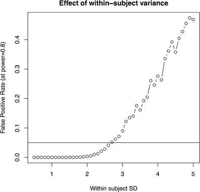
Figure 5. The effect of within subject variability on the ability to estimate group differences. This is estimated based on 10 subjects per group, four scans per subject.

FIGURE 6

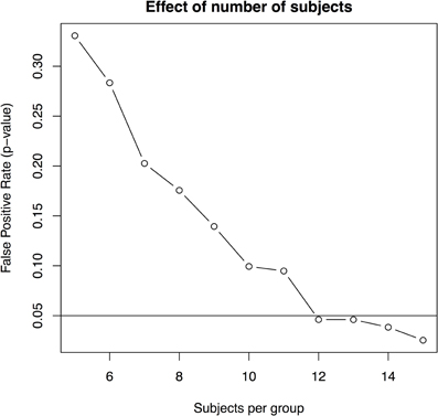
Figure 6. The effect of subjects per group based on a standard deviation of 3.1% and four scans per subject.

To generalize these data to other structures and situations, a more complete exploration of the parameter spaces is provided in Figures 7–9. In each case, the false positive rate (p-value) at a power of 0.8 is shown as a function of the subject and population standard deviations (Figures 7 and 8) or of the scans per subject and number of subjects (Figure 9). In comparison of Figures 7 and 8, there is a clear advantage to imaging in-vivo where population variance predominates, because each mouse can be fit with an independent intercept. Our hippocampal measurements, however, suggest this advantage is largely offset if relative volumes can be used instead of absolute volumes, as this significantly reduces the population variance (see dashed line, Figure 7).

FIGURE 7

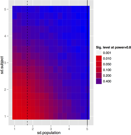
Figure 7. The trade-off between subject and population standard deviations (given in % volume) for the fixed-brain experiment. In the basic fixed-brain experiment we assumed that there was no subject variance (i.e., all within subject variance was methodological); if that is not true, then even the fixed-brain estimates will suffer. The black lines indicate standard deviations of absolute (solid) and relative (dashed) volumes as determined by our imaging data.

FIGURE 8

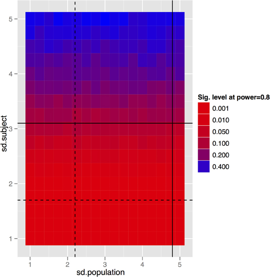
Figure 8. And the same tradeoff for the longitudinal in-vivo experiment. Clearly the population standard deviation has little effect, which is to be expected given that we are fitting a linear mixed effects model with a random intercept per subject. So the only variance we really care about is the within-subject variance. This simulation again assumes 10 subjects per group and four scans per subject. The black lines indicate standard deviations of absolute (solid) and relative (dashed) volumes as determined by our imaging data.

FIGURE 9

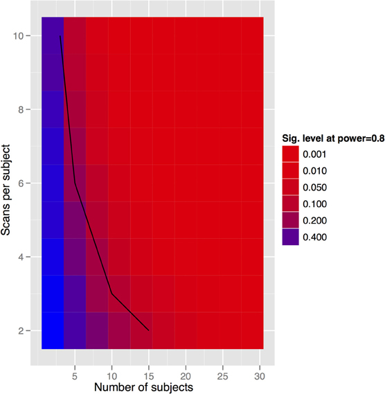
Figure 9. Tradeoff between scans per subject and subject numbers for the in-vivo experiment. Clearly we can get power by increasing either. The solid black line indicates the datapoints where the total scan number is kept to a constant 30 scans.

3.3. In-vivo Longitudinal Versus Cross-Section Ex-vivo Timecourse Experiments

Figure 10 explores the ability of both the in-vivo vs. ex-vivo experiments to accurately estimate the timecourse of hippocampal volume change. Here, the slope of the volume change over time is estimated and the total change over the time period estimated as the slope multiplied by the total time. We compare the in-vivo and ex-vivo situations keeping the numbers of scans constant; i.e., a longitudinal experiment with four scans each of 10 subjects is compared to a cross-sectional experiment with 40 different experimental subjects imaged with 10 at each of four timepoints. The density plots clearly show that the longitudinal data is better able to accurately estimate the slope and recover the 3% change in hippocampal volume when using either absolute or relative volumes (see also Table 3). However, again, the use of relative volumes provides a significant improvement in both the in-vivo and ex-vivo experiments, and very nearly eliminates the benefit of longitudinal in-vivo data.

FIGURE 10

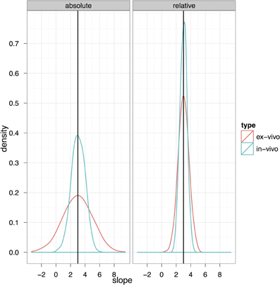
Figure 10. The ability to accurately recapture the slope in an in-vivo experiment with 10 subjects per group and four scans per subject (baseline plus three timepoints with an expected change) and a final expected change of 3% is shown here compared to a cross-sectional experiment with four similar timepoints but using ex-vivo acquisitions.

TABLE 3

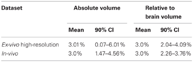
Table 3. The relative abilities of the in-vivo and high-resolution ex-vivo experiments to accurately estimate the slope (with an expected final change of 3%) of an induced change given as means and 90% confidence intervals (CI). See also Figure 10.

4. Discussion

There are multiple decisions that have to be made when designing a new mouse imaging study, including the choice of the number of animals to scan, whether to do a high-resolution fixed-brain experiment or, if imaging in-vivo, how many scans should be acquired for each animal over the duration of the experiment. Here we investigated these trade-offs by determining the source of variability in anatomy measurements derived from high field mouse MRI and then simulating an experiment designed to recover a subtle change in hippocampal volume.

One key conclusion from our imaging data is that anatomical variability in mouse imaging studies is low (∼5%), which is not surprising given that animals are typically from an inbred strain and raised in identical environments. Most of the variability in the population, moreover, is accounted for by the overall brain volume, and not specific to local structure volumes. For study design purposes, it is, therefore, important to note that the number of animals required to recover a change in relative (i.e., normalized) hippocampal volume is noticeably less than what would be required to recover estimated differences in absolute volumes.

In spite of the relatively low anatomical variability in inbred mouse populations, this variability remains the single most significant source of variance in imaging studies. Although the lack of a ground truth in our data makes it impossible to fully estimate the proportion of anatomical variance that is due to methods error vs. biological variance, repeatedly scanning the same specimen indicates that we can estimate hippocampal volume with a precision of approximately 1% with high-resolution ex-vivo imaging. Variability across a population of inbred mice, on the other hand, is around 5%, or 1.7% if brain volume is accounted for. This reiterates the tight correlation between volumes of a structure and total brain volumes. It is also likely to account for our observation that addition of extra subjects increases statistical power more efficiently than addition of imaging timepoints. Selection of additional subjects allows averaging of measurements across the population, where error is greatest.

We also noted, perhaps not surprisingly, that ex-vivo imaging provides greater precision than in-vivo imaging. For this reason, ex-vivo imaging will always be preferable when only detection of the anatomical phenotype is required, without attention to its timecourse. This is especially true if relative volumes are appropriate. However, longitudinal in-vivo experiments would be preferred where absolute volume measurements are required, including cases where many brain structures might be affected simultaneously, thus skewing measurements of the whole brain volume. Our data further suggest that longitudinal in-vivo experiments maintain a better ability to precisely estimate the rate of change across time than cross-sectional ex-vivo experiments, although this benefit is largely eliminated in cases where relative volume measurements are appropriate.

These results may be summarized in a few simple rules of thumb for mouse neuroimaging:

• relative volumes are more sensitive to anatomical phenotypes than absolute volumes and are appropriate if only perturbations to normal anatomy are expected;
• ex-vivo imaging at high-resolution is superior if a timecourse is not of interest;
• longitudinal in-vivo imaging is superior to cross-sectional ex-vivo imaging for measurement of changes in absolute volume and for characterizing the rate of change over time (although this advantage is nearly eliminated if relative volumes are appropriate); and
• addition of more subjects, rather than more timepoints, is preferred for improving the statistical power of a longitudinal study.

Of course, these rules are simplifications and there are several caveats to keep in mind when applying them. First, we considered specifically the volume of the hippocampus as our measurement of interest. The hippocampus is a relatively large structure in the mouse brain and can be effectively measured in both in-vivo and ex-vivo images. Other structures in the brain, and particularly smaller ones, may be very difficult to measure in-vivo, resulting in a much higher variance for the in-vivo data than is present in the hippocampus. This would favor use of ex-vivo imaging. The relative variances of structures of interest for both in-vivo and ex-vivo imaging must, therefore, be considered in design of the study. Second, other concerns, including limiting the numbers of mice used in research as well as potential uncertainty about the exact timing of the changes in neuroanatomy would suggest scenarios wherein fewer animals with more scans per animal are preferred. Other practical considerations, including limitations on the number of times mice can be scanned and the possibility of introducing confounding anatomical changes with repeated anesthesia, may ultimately determine the preferred design of any given experiment. In Mn-enhanced imaging experiments, in particular, possible toxicity due to repeated doses of Mn must be considered. While well-tolerated in adult rodents in single modest doses (∼80 mg/kg or less), repeated doses or exposure in early developmental stages will increase the likelihood of toxic effects (Gerber et al., 2002; Bock et al., 2008; Deans et al., 2008). This consideration favors the use of more subjects as opposed to more time points, a choice that our data suggests is statistically advantageous as well. On the other hand, the preparation of ex-vivo samples requires precise control over perfusion and fixation protocols in order to ensure consistency across all samples (Cahill et al., 2012), and will change the shape of the ventricular system due to a lack of cerebrospinal fluid pressure (Ma et al., 2008). Finally, it must be noted that we simulated a very simple linear change with a known beginning and end. Neither of these assumptions is likely to be perfectly true in any given experiment. Alterations in anatomy will not always be linear, nor will the precise timing of these changes always be known. While it would be possible to extend our simulations to encompass differing assumptions, the possible number of such combinations would provide a more complex set of rules.

In spite of the possible limitations of our study, we hope that the power analyses contained herein provide a guide for design of mouse imaging experiments. Increasingly, mouse imaging is providing insights into changes in the brain over time that cannot easily be visualized by any other means. We believe imaging will consequently be a powerful tool in understanding how the brain responds to stimuli and to disease. In combination with the genetic tools available in the mouse, this will present unique opportunities to understand the mechanisms of normal and pathological brain function. The guidelines in this manuscript will aid in design of these imaging studies, and in particular, suggest when in-vivo or ex-vivo study designs are likely to be most efficient.

Conflict of Interest Statement

The authors declare that the research was conducted in the absence of any commercial or financial relationships that could be construed as a potential conflict of interest.

References

Avants, B. B., Epstein, C. L., Grossman, M., and Gee, J. C. (2008). Symmetric diffeomorphic image registration with cross-correlation: evaluating automated labeling of elderly and neurodegenerative brain. Med. Image Anal. 12, 26–41.

Pubmed Abstract | Pubmed Full Text | CrossRef Full Text

Badea, A., Johnson, G. A., and Jankowsky, J. L. (2010). Remote sites of structural atrophy predict later amyloid formation in a mouse model of Alzheimer's disease. Neuroimage 50, 416–427.

Pubmed Abstract | Pubmed Full Text | CrossRef Full Text

Bock, N. A., Paiva, F. F., and Silva, A. C. (2008). Fractionated manganese-enhanced MRI. NMR Biomed. 21, 473–478.

Pubmed Abstract | Pubmed Full Text | CrossRef Full Text

Boyke, J., Driemeyer, J., Gaser, C., Büchel, C., and May, A. (2008). Training-induced brain structure changes in the elderly. J. Neurosci. 28, 7031–7035.

Pubmed Abstract | Pubmed Full Text | CrossRef Full Text

Cahill, L. S., Laliberté, C. L., Ellegood, J., Spring, S., Gleave, J. A., van Eede, M. C., Lerch, J. P., and Henkelman, R. M. (2012). Preparation of fixed mouse brains for MRI. Neuroimage 60, 933–939.

Pubmed Abstract | Pubmed Full Text | CrossRef Full Text

Carroll, J. B., Lerch, J. P., Franciosi, S., Spreeuw, A., Bissada, N., Henkelman, R. M., and Hayden, M. R. (2011). Natural history of disease in the YAC128 mouse reveals a discrete signature of pathology in Huntington disease. Neurobiol. Dis. 43, 257–265.

Pubmed Abstract | Pubmed Full Text | CrossRef Full Text

Chetelat, G. (2003). Early diagnosis of Alzheimer's disease: contribution of structural neuroimaging. Neuroimage 18, 525–541.

Pubmed Abstract | Pubmed Full Text | CrossRef Full Text

Collins, D. L., Holmes, C. J., Peters, T. M., and Evans, A. C. (1995). Automatic 3-D model-based neuroanatomical segmentation. Hum. Brain Mapp. 3, 190–208.

Collins, D. L., Neelin, P., Peters, T. M., and Evans, A. C. (1994). Automatic 3D intersubject registration of MR volumetric data in standardized Talairach space. J. Comput. Assist. Tomogr. 18, 192–205.

Pubmed Abstract | Pubmed Full Text

Deans, A. E., Wadghiri, Y. Z., Berrios-Otero, C. A., and Turnbull, D. H. (2008). Mn enhancement and respiratory gating for in utero MRI of the embryonic mouse central nervous system. Magn. Reson. Med. 59, 1320–1328.

Pubmed Abstract | Pubmed Full Text | CrossRef Full Text

Dorr, A. E., Lerch, J. P., Spring, S., Kabani, N., and Henkelman, R. M. (2008). High resolution three-dimensional brain atlas using an average magnetic resonance image of 40 adult C57Bl/6J mice. Neuroimage 42, 60–69.

Pubmed Abstract | Pubmed Full Text | CrossRef Full Text

Draganski, B., Gaser, C., Busch, V., Schuierer, G., Bogdahn, U., and May, A. (2004). Neuroplasticity: changes in grey matter induced by training. Nature 427, 311–312.

Pubmed Abstract | Pubmed Full Text | CrossRef Full Text

Driemeyer, J., Boyke, J., Gaser, C., Büchel, C., and May, A. (2008). Changes in gray matter induced by learning–revisited. PLoS One 3:e2669. doi: 10.1371/journal.pone.0002669

Pubmed Abstract | Pubmed Full Text | CrossRef Full Text

Gaser, G., and Schlaug, C. (2003). Gray matter differences between musicians and nonmusicians. Ann. N.Y. Acad. Sci. 999, 514–517.

Pubmed Abstract | Pubmed Full Text | CrossRef Full Text

Gerber, G. B., Léonard, A., and Hantson, P. (2002). Carcinogenicity, mutagenicity and teratogenicity of manganese compounds. Crit. Rev. Oncol. Hematol. 42, 25–34.

Pubmed Abstract | Pubmed Full Text

Hyde, K. L., Lerch, J., Norton, A. C., Forgeard, M., Winner, E., Evans, A. C., and Schlaug, G. (2009). Musical training shapes structural brain development. J. Neurosci. 29, 3019–3025.

Pubmed Abstract | Pubmed Full Text | CrossRef Full Text

Lau, J. C., Lerch, J. P., Sled, J. G., Henkelman, R. M., Evans, A. C., and Bedell, B. J. (2008). Longitudinal neuroanatomical changes determined by deformation-based morphometry in a mouse model of Alzheimer's disease. Neuroimage 42, 19–27.

Pubmed Abstract | Pubmed Full Text | CrossRef Full Text

Lerch, J. P., Carroll, J. B., Spring, S., Bertram, L. N., Schwab, C., Hayden, M. R., and Henkelman, R. M. (2008). Automated deformation analysis in the YAC128 Huntington disease mouse model. Neuroimage 39, 32–39.

Pubmed Abstract | Pubmed Full Text | CrossRef Full Text

Lerch, J. P., Sled, J. G., and Henkelman, R. M. (2011). MRI phenotyping of genetically altered mice. Methods Mol. Biol. 711, 349–361.

Pubmed Abstract | Pubmed Full Text | CrossRef Full Text

Lerch, J. P., Yiu, A. P., Martinez-Canabal, A., Pekar, T., Bohbot, V. D., Frankland, P. W., Henkelman, R. M., Josselyn, S. A., and Sled, J. G. (2011). Maze training in mice induces MRI-detectable brain shape changes specific to the type of learning. Neuroimage 54, 2086–2095.

Pubmed Abstract | Pubmed Full Text | CrossRef Full Text

Ma, Y., Smith, D., Hof, P. R., Foerster, B., Hamilton, S., Blackband, S. J., Yu, M., and Benveniste, H. (2008). In vivo 3D digital atlas database of the adult C57BL/6J mouse brain by magnetic resonance microscopy. Front. Neuroanat. 2:1. doi: 10.3389/neuro.05.001.2008

Pubmed Abstract | Pubmed Full Text | CrossRef Full Text

Montoya, A., Price, B. H., Menear, M., and Lepage, M. (2006). Brain imaging and cognitive dysfunctions in Huntington's disease. J. Psychiatry Neurosci. 31, 21–29.

Pubmed Abstract | Pubmed Full Text

Paulsen, J. S., Langbehn, D. R., Stout, J. C., Aylward, E., Ross, C. A., Nance, M., Guttman, M., Johnson, S., Macdonald, M., Beglinger, L. J., Duff, K., Kayson, E., Biglan, K., Shoulson, I., Oakes, D., and Hayden, M. (2008). Detection of Huntington's disease decades before diagnosis: the Predict-HD study. J. Neurol. Neurosurg. Psychiatry 79, 874–880.

Pubmed Abstract | Pubmed Full Text | CrossRef Full Text

Paulsen, J. S., Magnotta, V. A., Mikos, A. E., Paulson, H. L., Penziner, E., Andreasen, N. C., and Nopoulos, P. C. (2006). Brain structure in preclinical Huntington's disease. Biol. Psychiatry 59, 57–63.

Pubmed Abstract | Pubmed Full Text | CrossRef Full Text

Sawiak, S. J., Wood, N. I., Williams, G. B., Morton, A. J., and Carpenter, T. A. (2009). Voxel-based morphometry in the R6/2 transgenic mouse reveals differences between genotypes not seen with manual 2D morphometry. Neurobiol. Dis. 33, 20–27.

Pubmed Abstract | Pubmed Full Text | CrossRef Full Text

Scholz, J., Klein, M. C., Behrens, T. E. J., and Johansen-Berg, H. (2009). Training induces changes in white-matter architecture. Nat. Neurosci. 12, 1370–1371.

Pubmed Abstract | Pubmed Full Text | CrossRef Full Text

Silbert, L. C., Quinn, J. F., Moore, M. M., Corbridge, E., Ball, M. J., Murdoch, G., Sexton, G., and Kaye, J. A. (2003). Changes in premorbid brain volume predict Alzheimer's disease pathology. Neurology 61, 487–492.

Pubmed Abstract | Pubmed Full Text

Zakzanis, K. K., Graham, S. J., and Campbell, Z. (2003). A meta-analysis of structural and functional brain imaging in dementia of the Alzheimer's type: a neuroimaging profile. Neuropsychol. Rev. 13, 1–18.

Pubmed Abstract | Pubmed Full Text | CrossRef Full Text