 Zikuan Chen
 Zening Fu
 Vince Calhoun
- 1The Mind Research Network and LBERI, Albuquerque, NM, United States
- 2Department of Electrical and Computer Engineering, University of New Mexico, Albuquerque, NM, United States
Conventionally, brain function is inferred from the magnitude data of the complex-valued fMRI output. Since the fMRI phase image (unwrapped) provides a representation of brain internal magnetic fieldmap (by a constant scale difference), it can also be used to study brain function while providing a more direct representation of the brain's magnetic state. In this study, we collected a cohort of resting-state fMRI magnitude and phase data pairs from 600 subjects (age from 10 to 76, 346 males), decomposed the phase data by group independent component analysis (pICA), calculated the functional network connectivity (pFNC). In comparison with the magnitude-based brain function analysis (mICA and mFNC), we find that the pFNC matrix contains fewer significant functional connections (with p-value thresholding) than the mFNC matrix, which are sparsely distributed across the whole brain with near/far interconnections and positive/negative correlations in rough balance. We also find a few of brain rest sub-networks within the phase data, primarily in subcortical, cerebellar, and visual regions. Overall, our findings offer new insights into brain function connectivity in the context of a focus on the brain's internal magnetic state.
Introduction
Phase functional magnetic resonance imaging (fMRI) is an MRI technique dedicated to fMRI phase data acquisition and post-acquisition processing and analysis. In principle, an fMRI study produces a timeseries of complex-valued images consisting of pairwise magnitude and phase components; therefore, the fMRI phase data are generated together with the magnitude data in an fMRI experiment (at no extra cost). Since the complex-valued fMRI data (magnitude and phase images in pairs) are formed from the same magnetic source (the internal inhomogeneous magnetic fieldmap) through intravoxel dephasing signal detection and subsequent complex modulo/argument calculations (Chen and Calhoun, 2015b), both are useful for brain function depiction with different representations (in different measurements). In theory, the fMRI phase data are more suitable for brain function analysis since phase imaging represents the brain magnetic state seen in internal magnetic fieldmaps.
There is a body of reports on the exploration and exploitation of phase fMRI for brain function study (Rowe, 2005, 2009; Arja et al., 2009; Feng et al., 2009; Balla et al., 2014; Bianciardi et al., 2014; Chen and Calhoun, 2016b; Ozbay et al., 2016). Under linear imaging conditions, an fMRI phase image represents the brain internal magnetic field distribution captured at a timepoint (Chen and Calhoun, 2015b; Chen et al., 2018b). This portrays a brain magnetic state (a magnetization state in a main field B0, in preparation for MRI scanning) during brain activity (Shmueli et al., 2009; Li et al., 2011; Chen and Calhoun, 2013, 2015a; Wang and Liu, 2015).
In theory, the fMRI magnitude signal is calculated from the complex signal by a nonnegative nonlinearity (e.g., |±1| = 1) that fails to represent the source of an internal fieldmap (e.g., degenerating the signs associated with the bipolar-valued field distribution). In comparison, the fMRI phase signal is calculated from the complex MRI signal through a trigonometric operation, arctan(φ), which can be linearly approximated by arctan(φ) ≈ φ for |φ| < 1 (φ denotes a phase signal, measured in units of radian, related to the field value by a constant scale γTE). Therefore, a phase image is linearly related to the magnetic field in linear phase fMRI (Haacke et al., 1999; Chavhan et al., 2009; Chen and Calhoun, 2015b, 2016b). We may infer the internal fieldmap source from an fMRI phase image under linear approximation; however, such inverse mapping is not available from fMRI magnitude data (due to an irreversible magnitude nonlinearity like |±1| = 1).
The trigonometric arctan(φ) gives a good linearization for a very small φ, as mathematically defined by arctan(φ) = φ for |φ| < < 1. In order to maximally reduce the nonlinearity associated with arctan(φ), we adopt an additive perturbation model, φ(t) = φ0 ± δφ(t), to extract the BOLD-only phase signal (the perturbation term δφ(t)) from a timeseries of BOLD phase signals through complex division (a Hilbert inner product) (Chen and Calhoun, 2016b; Chen et al., 2018b). The BOLD-only phase signal δφ results in good linear mapping of the source of BOLD-only magnetic field perturbation by reducing the nonlinearity associated with arctan(φ).
Given a timeseries of fMRI images, we can break down brain function into a collection of brain subfunctions (subnetworks) through an independent component analysis (ICA) method (Calhoun et al., 2001; McKeown et al., 2003; Guo and Pagnoni, 2008; Calhoun and Adali, 2012). Taking advantage of data-driven multivariate statistics, the ICA method has been successfully extended to allow population-level group data analysis (a technique of group ICA) (Calhoun et al., 2001; Beckmann et al., 2005; Guo and Pagnoni, 2008; Calhoun and Adali, 2012). Accordingly, we can apply group ICA to magnitude and phase data separately for brain function decompositions, as denoted by mICA and pICA (Chen et al., 2018a). For comparison of mICA and pICA in correspondence, we constrain the pICA with the magnitude-inferred group information and implement group-information-guided (GIG) pICA (Du and Fan, 2013).
Using mICA and pICA, we then calculate their functional network connectivity (FNC) matrices (denoted by mFNC and pFNC) based on the temporal correlation of mICA and pICA timecourses (Jafri et al., 2008; Arbabshirani and Calhoun, 2011). For larger population data analysis, we may discard the insignificant functional connections based on statistical significance (based on p-value assessment). For example, a p-value thresholding (<10−10) removes insignificant connections in mFNC, enhancing identification of significant whole-brain connections such as sparsity, balance, and near and far couplings.
We have recently reported on a method of comparing magnitude and phase-based brain functional connectivity in the resting state via statistical analysis over 100 subjects (Chen et al., 2018a). This revealed interesting similarities and distinctions between mFNC and pFNC. Here, we used a larger cohort of subject data (N = 600) to analyze the brain functional connectivity patterns in mFNC and pFNC matrices. We addressed the following aspects: intra-domain (short-range, near) and inter-domain (long-range, far) connections, positive and negative connections, sparseness and nonuniformity of connection distribution, and robustness and significance of group-level connections.
Methods
Data Collection
A collection of 600 subject datasets (in pairs of magnitude and phase images) were acquired from a cohort of participants (age: 10–76 years, 346 male/254 female) by subject scanning in a Siemens TrioTim 3T scanner at the Mind Research Network. Informed consent was obtained for each subject and the subject scanning protocol was approved by the IRB at the University of New Mexico. The data were gained from the subjects anonymously prior to group analysis.
The fMRI experiments were performed with the following parameter settings: 12-channel coil, GRE-EPI sequence, TE = 29 ms, TR = 2 s, flip angle = 75°, field of view = 240 cm × 240 cm, matrix size = 64 × 64, voxel size = 3.75 mm × 3.75 mm × 4.55 mm, slice thickness = 3.5 mm, slice gap = 1.05 mm, total slices 33, acquisition time (TA) = 5 min, and total volumes 150. Subjects were instructed to keep their eyes open during the scanning and fixate on a foveally presented cross. We obtained two groups of fMRI data, using magnitude and phase images in pairs, with each in a 4D format (64 × 64 × 33 × 150, 3D spatial and 1D temporal in dimension).
Data Processing
Preprocessing the fMRI magnitude images included removing the first two timepoints to avoid T1 equilibration effects; realignment using INRIalign; slice-timing correction using the middle slice as the reference frame; spatial normalization into MNI space with resampled isotropic voxels (3 × 3 × 3 mm); and spatial smoothing with a Gaussian kernel (FWHM = 9 mm). Through data processing, each 4D subject data (magnitude and phase separately) in 64 × 64 × 33 × 150 format was converted to 53 × 63 × 46 × 148. For fMRI magnitude image preprocessing, we used the SPM8 automated pipeline (Chen et al., 2018a) as reported (http://www.fil.ion.ucl.ac.uk/spm/software/spm8/).
Extracting BOLD-Only Phase Signals
The raw phase images were first converted to a range in radian (–π, π) and denoted by φ (bipolarly valued). Then, the phase series images were subjected to spatial realignment through the 3D affine transformation using the motion correction parameters (4 × 4 affine transformation) as derived from the magnitude image realignment in the corresponding magnitude timeseries. Upon phase timeseries image realignment, a complex division (Equation A2 in Appendix) was used to extract the temporal phase changes (BOLD-only phase response) with respect to the middle frame at the middle timepoint in the series (Chen et al., 2018b), as denoted by δφ (bipolarly valued). This calculation is a time-domain phase-unwrapping technique that can extract the small temporal phase changes (< < π) buried in phase-wrapped timeseries signals (Chen and Calhoun, 2016b). Using the phase image processing, we obtained a 4D phase data δφ(r,t) for each subject in a format of 53 × 63 × 46 × 148.
Group mICA and GIG-pICA
The SPM-processed magnitude data were decomposed into functional networks using a group-level spatial ICA as illustrated (Chen et al., 2018a) and implemented in the GIFT toolbox (http://mialab.mrn.org/software/gift/). We decomposed the group magnitude data into a number of 100 brain subfunctions (a relatively high model order brain functional ICA), denoted by mICA. The Infomax spatial ICA algorithm was repeated 10 times in ICASSO (http://www.cis.hut.fi/projects/ica/icasso). The aggregate spatial maps were estimated as modes of spatiotemporal ICA(r, t). Subject-specific spatial maps {mICA j(r)} and timecourses {mICAj(t))} (j = 1, 2, …, 600) were estimated using a back-reconstruction method (Calhoun et al., 2001; Erhardt et al., 2011). Then, we selected a subset of 50 components (intrinsic connectivity networks) from the 100 plenary by excluding mICAs obviously affected by physiological, motion, and imaging artifacts as characterized by noncortical activation in spatial maps and high-frequency fluctuations in timecourses (Beckmann et al., 2005; Allen et al., 2011, 2014).
The timecourses mICA(t) underwent postprocessing that included (1) detrending, (2) removing outliers, and (3) low-pass filtering with a cutoff frequency at 0.15 Hz. Finally, the postprocessed mICA(t) were normalized to have a unit variance such that the covariance matrices correspond to correlation matrices (Allen et al., 2014).
Considering the mICA as the brain functional template for group information guidance, we conducted brain functional decomposition on the group phase data δφ using the GIG-ICA method (Du and Fan, 2013), thus implementing GIG-pICA. We use the GIG-ICA method for phase data decomposition for two reasons: (1) facilitating mICA and pICA correspondence and comparison; and (2) in comparison with the direct ICA phase data decomposition (in our previous 100-subejct experiment Chen et al., 2018a) to show the convergence in phase-inferred features; for example, both pICA methods produce functional cliques in subcortical region.
The pICA timecourses were then postprocessed in ways similar to the mICA timecourse postprocessing. As a result, we obtained a set of 50 pICA components in counterpart to the 50 mICA components.
Group mFNC and Group pFNC Matrices
According to brain structure and functional organization, we classified the 50 selected mICA components roughly into seven brain domains based on spatial activation locations, as ordered by subcortical region (SC(4)), auditory (AUD(2)), sensorimotor (SM(8)), vision (VIS(10)), cognitive control (CC(14)), default mode network (DMN(9)), and cerebellum (CB(3)).
An aggregate ICA timecourse was back-reconstructed using data from 600 subjects to generate the same number of individual subject ICA timecourses. For each subject, we calculated a temporal correlation matrix (i.e., producing a subject-specific FNC matrix). In the results, we obtained 600 single-subject {mFNCj} and {pFNCj} matrices, j = 1, 2, …, 600, for magnitude and phase data, respectively. We converted the entries in {mFNCj(n1, n2)} and {pFNCj(n1, n2)} matrices (in size of 50×50×600) to Fisher z-scores (via a Matlab routine atanh(x)). By averaging the assemblies, we obtained group-level mFNC and pFNC matrices (in size of 50×50).
Null-Hypothesis Tests on Group mFNC and pFNC
An entry at (n1, n2) in mFNC(n1, n2) matrix represents a specific functional connection between subfunction mICAn1 and subfunction mICAn2, for n1, n2 = 1, 2, …, 50. All the entry values collected from the 600 subject-specific connections constitute an assembly of 600 samples. Through a one-sample t-test (on the null hypothesis that an entry at (n1, n2) in the group-level mFNC matrix assumes a zero-mean distribution across the 600 samples {mFNCj}), we obtained a p-value and an H-rest value. From all of the t-tests on the assembly {mFNCj(n1, n2), j = 1, 2,…, 600, n1, n2 = 1, 2,…,50}, we obtained a p-value matrix PmFNC (n1, n2) in a value range [0,1] and a H-test matrix HmFNC(n1, n2) (binary valued {1,0}), in size of 50 × 50. In the same procedure, we obtained a p-value matrix PpFNC and an H-test matrix HpFNC from the phase data assembly {pFNCj}. Each entry of the p-value matrix was calculated from a statistic t-test over the 600 subject-specific FNCs with a confidence interval. The confidence intervals associated with the p-value matrix calculation may vary from entry to entry, which may assume different bounds delimited by positive and negative values.
The statistical hypothesis test may mistakenly produce some rejections of null hypothesis (zero mean), which we can control using the false discovery rate (FDR) through a FDR correction procedure (Benjamini and Hochberg, 1995; Benjamini and Yekutieli, 2001, 2005). This is a more powerful method for correcting FDR for multiple comparisons than the standard Bonferroni correction. It offers a strong control of the family-wise error rate (i.e., the probability that one or more null hypotheses are mistakenly rejected). The FDR correction leads to adjusted p-values. We made FDR corrections on PmFNC and PpFNC for a specified desirable FDR (default p = 0.05).
Based on the binary HmFNC(n1, n2) (H = 1 for zero-mean rejection, H = 0 for zero-mean accepted at the 5% level), we excluded the functional connections that have zero-mean distributions (entries with H = 0). We focused on the connections in mFNC(n1,n2) whose entries take on nonzero-mean distributions (determined by H = 1). We edited pFNC(n1, n2) based on the binary HpFNC(n1, n2).
Numerical Characteristics of mFNC and pFNC
Based on the FDR-corrected p-value matrices, PmFNC and PpFNC, we assessed the significance and robustness of the functional connections through a p-value thresholding as given by
where pthresh denotes a specified p-value (pthresh = 0.05 for the default statistics significance) and the superscript “<” denotes a smaller-than p-value thresholding. As pthresh decreases, the p-value thresholding produces a smaller number of survival entries (≠ 0) in mFNC< and pFNC< matrices, representing the sparsity of higher significant functional connections; high significant connections are also strong connections.
For comparative pattern analysis of matrices mFNC< and pFNC<, we expect the following characteristics:
(1) Statistically significant connections through p-value thresholding in Eq. (1a,1b) with a span of pthresh = {0.05, 10−10, 10−50, 10−100, 10−150, 10−200}.
(2) Positive/negative connections and connectivity balance in terms of mean(FNC) ± std(FNC) (Chen et al., 2018a). The connectivity balance can be also be characterized by the entry number difference between positive count (denoted by #(+)) and negative count (denoted by #(-1)) of signs in mFNC< or pFNC<.
(3) Intra-domain (near, in a diagonal block) and inter-domain (far, in an off-diagonal submatrix) connections.
(4) Sparseness and nonuniformity of significant connections. The sparsity can be numerically characterized by the small fractions #(+)/1225 and #(-)/1225, where 1225 = 50(50-1)/2 is the number of total entries in a symmetrical 50 × 50 matrix excluding the self-connections on the diagonal line. The nonuniformity is visibly inspected in mFNC< and pFNC< as some submatrices disappear while some other submatrices persist during the p-value thresholding.
Results
Group mFNC and pFNC
Considering ICA components as coherent brain functional networks, we calculated the functional network connectivity matrix by the temporal correlations (Pearson correlations) among the ICA timecourses. In Figures 1A,B are shown the magnitude and phase-depicted mFNC and pFNC matrices (in size 50 × 50), as calculated by the average over the subject-specific {mFNCj(n1, n2)}and {pFNCj(n1, n2)} matrices, respectively. Note the 50 mICA components were arranged in seven domains: SC(4), AUD(2), SM(8), VIS(10), CC(14), DMN(9), and CB(3), as shown at the left vertical labels in Figure 1A. Correspondingly, the 50 pICA components were arranged with the same labels in Figure 1B.
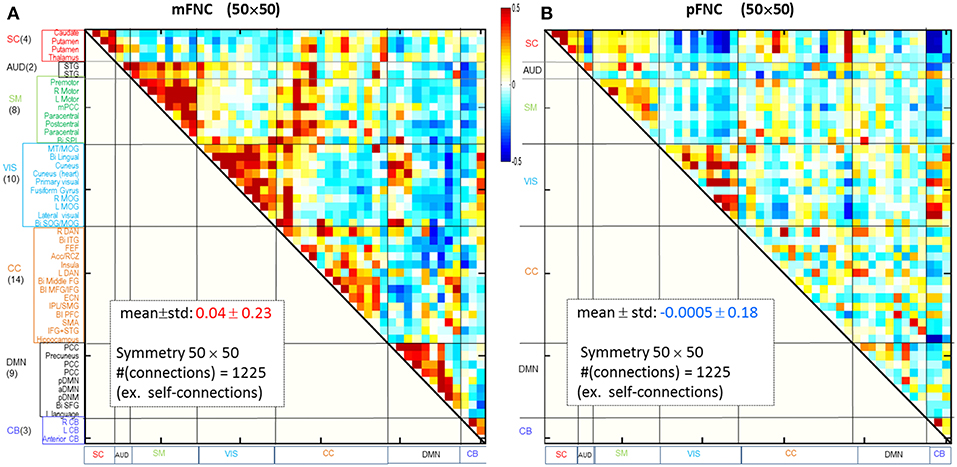
Figure 1. Brain resting-state subfunction arrangement and functional network connectivity. (A) Magnitude data depiction: a set of 50 mICA components are classified into seven (7) brain domains {SC(4), AUD(2), MOT(8), VIS(10), CC(14), DMN(9), and CB(3)} and the mFNC matrix (mean ± std: 0.04 ± 0.23); (B) Phase data depiction: the pICA components are classified into 7 domains and the pFNC matrix (mean ± std: −0.0005 ± 0.18).
The ICA-decomposed brain subfunctions are distributed over the brain geometrical space partitioned in seven domains. In general, the intra-domain connections are short connections, whereas the inter-domain connections are always long connections (except for rare inter-domain connections at the domain boundary). In an FNC matrix, an intra-domain short-range (near) connection constitutes the on-diagonal blocks and an inter-domain long-range (far) connection is located in the off-diagonal regions. In Figure 1, the magnitude data show strong positive near couplings in the on-diagonal blocks (Figure 1A), which differs from the phase-depicted loose connections (Figure 1B).
One Sample t-tests of Group-Level mFNC and pFNC
The group-level mFNC and pFNC matrices were calculated using an average from assemblies {mFNCj} and {pFNCj}, respectively. The t-test on the mFNC matrix gives rise an H-test matrix HmFNC and a p-value matrix PmFNC (in size of 50 × 50), as shown in Figures 2A,C. The averaged confidence interval for PmFNC is [0.02, 0.06]. Meanwhile, the pFNC t-test gives rise to HpFNC and PpFNC, as shown in Figures 2B,D. The averaged confidence interval for PpFNC is [−0.02, 0.02]. Note that the p-value matrices were displayed in a magnification by log10. The binary H-test matrices were interpreted as H = 1 for rejecting null hypothesis (nonzero mean distributions) and H = 0 for true null hypothesis (zero mean distributions).
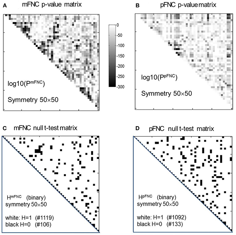
Figure 2. One-sample t-tests for the assemblies {mFNCn} and {pFNCn} (n = 1,2,…,600). (A,B) The t-test p-value matrices (displayed by a log10 magnification) using PmFNC(50,50) for {mFNCn} and PpFNC(50,50) for {pFNCn}; (C,D) The null-hypothesis test results (the entries with H = 1 were used for connection significance analysis).
In Figure 2C, there are 1,119 entries (H = 1 for significant connection) and 106 entries (H = 0 for noisy or random connection) in the H-test matrix HmFNC (50 × 50, with a total number of 1,225 entries in the upper triangle). In Figure 2D, there are 1,092 entries (H = 1) and 133 entries (H = 0) in the H-test matrix HpFNC. The entries with H = 0 usually take on small values in mFNC and pFNC matrices, which we consider as noise and omit accordingly (by resetting them to zeros).
Thresholding mFNC and pFNC
We assessed the statistical significance of the functional connections in FNC matrices based on p-value thresholding in Equations (1a,b). In Figure 3, the thresholded matrices (mFNC<) are drawn from p-value thresholding with pthresh = {0.05, 10−10, 10−50, 10−100, 10−150, 10−200} using the upper triangle portions of the symmetric matrices. For each mFNC< matrix (after FDR correction), we calculated the following characteristics: mean ± std, the number of positive couplings (#(+)), the sum of positive couplings (∑(+)), the number of negative couplings (#(–)) and the sum of negative couplings (∑(–)). The connectivity balance can be characterized as mean(mFNC<). We can also quantify the functional connectivity imbalance by the quantity #(+) – #(–) in mFNC< or alternatively by ∑(+) – ∑(–).
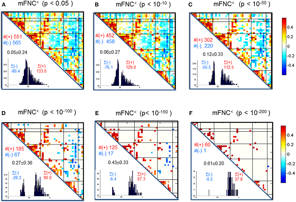
Figure 3. (A–F) Significant connections in group mFNC matrix under p-value thresholding with pthresh = {0.05, 10−10, 10−50, 10−100, 10−150, 10−200}. The numbers of positive and negative connections (denoted by #(+) and #(–) respectively), and the sums of positive and negative connections (denoted by ∑(+) and ∑(–) respectively) were calculated from the survival entries in the pthresh-thresholded matrices (mFNC<).
Correspondingly, in Figure 4 we show the thresholded pFNC matrices using the same p-value thresholdings and numerical characterizations {#(+), #(–), ∑(+), ∑(–)} as used for mFNC. In Figure 4E, the subcortical nuclei (SC) reveal significant negative couplings with VIS and CB, along with significant positive couplings with CC (p < 10−150).
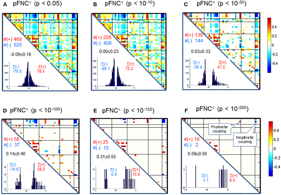
Figure 4. (A–F) Significant connections in group pFNC matrix under p-value thresholding with pthresh = {0.05, 10−10, 10−50, 10−100, 10−150, 10−200}. The numbers of positive and negative connections (denoted by #(+) and #(–) respectively), and sums of positive and negative connections (denoted by ∑(+) and ∑(–) respectively) were calculated from the survival entries in the pthresh-thresholded matrices (pFNC<).
In Figure 5, we present the magnitude- and phase-depicted whole-brain connectivity behaviors for significant connections as determined by p-value thresholding. Specifically, we show the plots on the numerical characteristics (in terms of mean, counts of positive and negative connections (#(+), #(–)), and sums of positive and negative connections (∑(+), ∑(–)) of mFNC< and pFNC< matrices under p-value thresholding with pthresh = {0.05, 10−10, 10−50, 10−100, 10−150, 10−200.}. In Figure 5A, we show the whole-brain connection balance in terms of mean(mFNC<) and mean(pFNC<), in which a large mean value indicates a connection imbalance (deviation from balance 0). In Figure 5B, we use the average of whole-brain connection strength in terms of mean(|mFNC<|) and mean(|pFNC<|), in which a large value indicates a strong connection. It is noted that for small mean(mFNC) and mean(pFNC) values (close to 0), we may use the std(mFNC) and std(pFNC) values to quantify connection strengths instead what was used in (Chen et al., 2018a). In Figures 5C,D, we show the positive and negative numbers (#(+) vs. #(–)) in mFNC< and pFNC< matrices with respect to the p-value thresholding, where the difference #(+) – #(–) can be used to quantify the whole-brain connection imbalance. In Figures 5E,F, we also the show the positive and negative connections in terms of ∑(+) and ∑(–) with respect to pthresh, where the difference ∑(+) – ∑(–) can also be used to evaluate the connection imbalance. Overall, our experimental results in Figure 5 show in comparison with fMRI magnitude data usage that the fMRI phase data reveal more connection balance (mean(pFNC<) < mean(mFNC<)) in Figure 5A, higher connection strength (mean(|pFNC<|) > mean(|mFNC<|)) in Figure 5B, and more balance in positive and negative distributions as determined by a smaller #(+) – #(–) in Figures 5C,D. and a smaller ∑(+) – ∑(–) in Figures 5E,F.
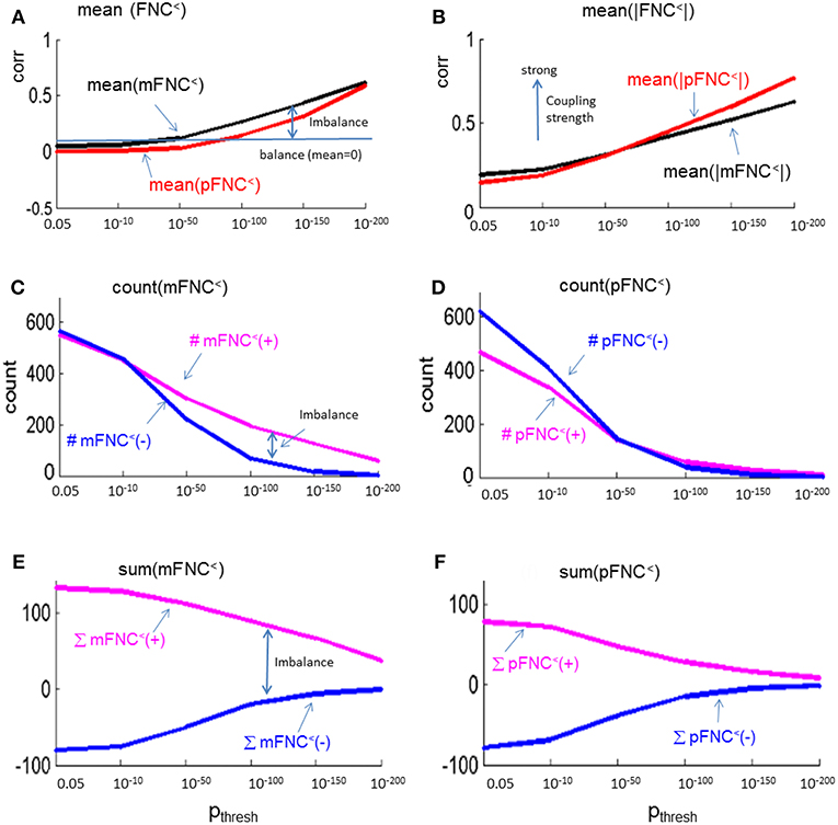
Figure 5. Numerical characteristics of mFNC and pFNC under p-value thresholding. (A) mean(mFNC<) and mean(pFNC<) whole-brain network balance; (B) mean(|mFNC<|) and mean(|pFNC<|) whole-brain network coupling strength; (C) Counts of positive and negative couplings in mFNC<; (D) Counts of positive and negative couplings in pFNC<; (E) Sums of positive and negative couplings in pFNC<; and (F) Sums of positive and negative couplings in pFNC<.
Significant Couplings in mFNC
We used p-value thresholding on mFNC to examine robustness and significance of the magnitude-depicted brain functional connections for whole brain space in resting state (Figure 3). Here, in Figure 6, we see significant connections survived in a very strong p-value thresholding (p < 10−200, Figure 3F). Specifically, we show in Figure 6A the functional connections across the seven domains (MOT(8), CC(14), AUD(2), DMN(9), SC(4), CB(3), VIS(10) in an arrangement around a circle) along with links of intra-domain (all are positive, in bright red), positive inter-domain (in dim red), and negative inter-domain (in blue). We observed the following aspects: (1) there are 60 positive connections and 1 negative connection; (2) the domains (MOT, VIS, DMN) each contain dense intra-domain connections; (3) there is no inter-domain connection between (MOT, VIS), (DMN,CC), (DMN, AUD), (DMN, SC), (DMN, CB), (SC, CB), (AUD, SC), and (AUD, CB); and (4) there is no intra-domain link in CB. In Figure 6B, we displayed the only negative connection survived in p < 10−200 during brain resting state, which shows the inter-domain connection between (CC, CB) in a connection strength 0.41 (p = 2 × 10−209). Obviously, the magnitude depicted high significant connections in Figure 6 (p < 10−200) in resting brain state are nonuniformly distributed over the brain space: dense connections in VIS, MOT, and DMN, sparse connections in CC and SC, and no connections within CB.
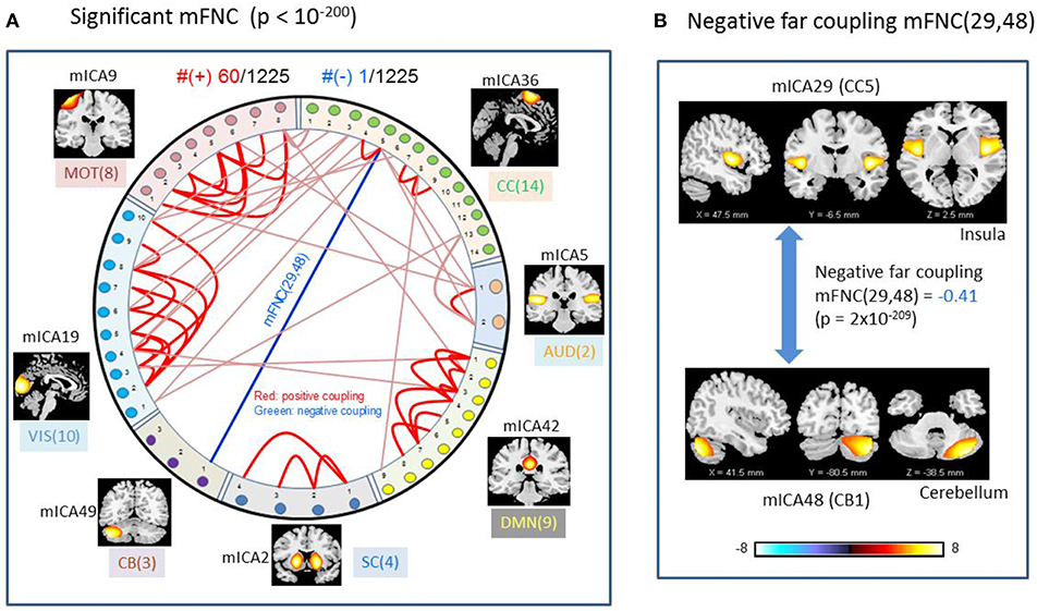
Figure 6. Illustrations of the most significant couplings in mFNC< (p < 10−200). (A) There are 36 intra-domain positive couplings (near, in bright red color) and 18 inter-domain positive couplings (far, in soft red color), and 1 inter-domain negative coupling (far, in blue color). (B) Features of the negative interdomain coupling mFNC(29, 48).
Significant Couplings in pFNC
In comparison with the most significant connections in mFNC in Figure 6, we scrutinize the phase-depicted significant connections in mFNC under the same p-value thresholding (p-value < 10−200) in Figure 7. We observed the following aspects: (1) there are a few connections survived in p-value < 10−200 (10 positive connections and 2 negative connections); (2) there is no intra-domain connections in MOT,CC, AUD, DMN; (3) there are 2 negative far inter-domain connections between (CB, SC); (4) there is 1 positive far inter-domain connection between (CC, SC); (5) there are no inter-domain connections among {MOT, CC, AUD, DMN, VIS, CB}; and (6) only SC has inter-domain connections (1 with CC, 2 with CB). In Figure 7B, we displayed the connections among {SC1(pICA1),SC3(pICA3),CB1(pICA48)}, which assume 2 negative far inter-domain connections and 1 positive near intra-domain connection. The subcortical subfunction SC1(pFNC1) is strongly coupled with SC3(pFNC3) with pFNC(1,3) = 0.80 and a high significance (p-value = 8 × 10−250), which constitutes a functional clique in the subcortical nuclei. It seems plausible for the phase data analysis to show that the subcortical nuclei (consisting of basal ganglia and thalamus) form a functional clique that acts as a hub in couplings with other cortical subfunctions in the resting state. This observation is consistent with our previous report on the functional subcortical clique observed from a 100-subject rest fMRI experiment (Chen et al., 2018a).
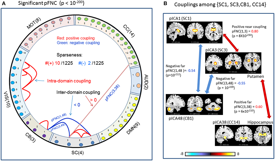
Figure 7. Illustrations of the most significant couplings in pFNC< (p < 10−200). (A) There are nine (9) intra-domain positive couplings (near, in bright red color) and one (1) inter-domain positive coupling (far, in soft red color), and two (2) inter-domain negative couplings (far, in blue color). (B) Features of the two negative interdomain couplings pFNC(1,48) and pFNC(3, 48).
Discussion
Inferring BOLD-Only Internal Magnetic Field Perturbation From Phase MRI
The rationale of phase fMRI for brain function study lies in the fact that we can infer the brain internal magnetic field distribution from an fMRI phase image under linear approximation (a small phase angle condition). For reference convenience, we provide the approximation theory of phase-to-field inverse mapping in the Appendix. An fMRI phase image represents a snapshot capture of the brain magnetic state (in terms of magnetic field distribution) under linear phase fMRI approximation. A voxel phase signal represents an intravoxel-average magnetic field value.
As seen in Equation (A3), phase fMRI procures a phase image φ from the MRI quadrature detection by a trigonometric operation, arctan(φ), which is nonlinear in a general setting. Mathematically, we have a linear approximation, arctan(φ) = φ for |φ| < < 1 radian (a small phase angle condition). Numerical simulation (Chen and Calhoun, 2015b) has shown that the phase fMRI nonlinearity (arctan(φ)) is weak for large phase angles (|φ| ~ π rad). In reality, an fMRI phase image always has phase wrapping due to the dominant phase background (|φ0| > π radian). In practice, an unwrapped phase image is always assumed to represent the internal magnetic fieldmap with the associated nonlinearity of large phase angles (|φunwrap| > π).
For fMRI data analysis, we extract the dynamic phase perturbations (δφ) using a complex-division approach in Equation (A8), which are considered the BOLD-only phase response signals during a brain activity. Then we infer the BOLD-only magnetic field perturbation (δb) by a linear scaling mapping in Equation (A9). The small phase perturbation (typically |δφ| < 0.2 radian) ensures a good linear approximation: arctan(δφ) = δφ for |δφ| < < 1. Note that we cannot infer the brain magnetic fieldmap from magnitude fMRI due to irreversible nonlinearity.
Bipolar-Valued Brain Magnetic Field Distribution
A magnetic field may assume positive and negative values. For brain fMRI study, the brain internal magnetic field is from a brain tissue magnetization in a main field B0. Specifically, this brain tissue magnetic susceptibility property (denoted by χ) undergoes a dipole-convolved magnetization in B0 to establish an inhomogeneous magnetic fieldmap. Due to the spatial derivative property of the dipole kernel, even a nonnegative susceptibility distribution (χ ≥ 0) could induce a bipolar-valued fieldmap (Chen et al., 2018b). The negative signs in a χ-induced fieldmap are maintained during the forward phase fMRI, which result in the fieldmap reconstruction by an inverse mapping from phase to fieldmap. In comparison, the negative signs are completely suppressed (inverted) in the fMRI magnitude signals due to its nonnegativeness (Chen and Calhoun, 2011). In this sense, the phase fMRI provides a direct, accurate representation of the brain magnetic state for bipolar-valued magnetic fieldmaps. Nevertheless, the magnetic fieldmap still differs from the underlying brain tissue magnetic susceptibility map using a 3D dipole convolution (Chen and Calhoun, 2013), which in principle can be completely resolved through functional quantitative susceptibility mapping (fQSM) or functional susceptibility mapping (Balla et al., 2014; Chen and Calhoun, 2015a, 2016a,c). More accurate brain functional connectivity analysis using original magnetic susceptibility source data is an important research in future.
Positive and Negative Functional Connections
Research has shown positive and negative functional connections exist among ICA-decomposed brain networks (subfunctions) (Xu, 2015; Xu et al., 2015), either in the resting state or in task performance. Most reports on balanced connectivity (Marino et al., 2005; Fox et al., 2009; Murphy et al., 2009; Litwin-Kumar and Doiron, 2012; Liu et al., 2015) were based on fMRI magnitude data analysis in which the negative magnitude connections (anticorrelations) were reported as a result of a “de-mean” preprocessing that is prone to artifactual negative connections. Using bipolar-valued fMRI phase data, we found more negative connections that cancel the positive connection(s) to make a balanced network for the whole-brain functional connectivity without a de-mean preprocessing (Chen et al., 2018a).
Overall, the phase-depicted balanced brain functional connectivity draws from the bipolarity of phase signals (Figure 1B), while magnitude-depicted positively-biased connectivity stems from the nonnegative magnitude signals (Figure 1A). These observations are consistent with our previous report with a 100-subject experiment data analysis (Chen et al., 2018a). Since the linear inverse mapping from fMRI phase to magnetic fieldmap maintains the negative signs, the δb-depicted negative connections come from negative phase signals and anti-correlations.
Near and Far Functional Connections
The magnitude-based brain functional connectivity study (Rosenbaum et al., 2017) has shown that nearby neurons are positively correlated, pairs at intermediate distances are negatively correlated, and distant pairs are weakly correlated. We found similar connection patterns in mFNC (Figure 1A): the on-diagonal positive blocks indicate strong near (intra-domain) connections, while off-diagonal blocks have negative and small values indicating weak far (inter-domain) connections.
In comparison, the phase-based brain function connectivity in pFNC (in Figure 1B) reveals some different patterns. Figure 1B reveals negative near connections within domains VIS, CC, and DMN in small and negative entries in the on-diagonal blocks; also seen are off-diagonal negative and positive blocks indicating strong far (inter-domain) connections. In particular, the subcortical subfunctions (SC(4)) show strong negative connections with both the visual subfunctions (VIS(10)) and the cerebellum subfunctions (CB(3)), while the VIS(10) are generally positively connected with CB(3).
Sparseness and Nonuniformity of Brain FNC
Given a set of ICA-decomposed brain subfunctions, the whole-brain functional connectivity is numerically characterized in an FNC matrix (e.g., mFNC from magnitude data and pFNC from phase data). An entry value in the FNC matrix represents the correlation between two subfunctions in a range [−1, 1]: a large value (~1) indicates a synchrony and a negative sign an anti-correlation. The entries with small values (~0) are largely due to noise (randomness and instability). For brain function connectivity depiction, we are concerned with the strong connections (negative or positive) over the brain space (near or far connections). By omitting the entries in small values (i.e., via thresholding like Equation 1), we have a small number of survival entries in the FNC matrix showing the sparseness (counting entries in a thresholded FNC matrix) and nonuniformity of their distribution over the brain space.
In our experiment, we had a large number of subject data (N = 600) for statistical brain function study. Based on the FNC assemblies {mFNCj} and {pFNCj}, we conducted t-tests on the group-level functional connections to obtain p-value matrices, PmFNC and PpFNC, and H-test matrices, HmFNC and HpFNC, respectively. We omitted the entries in mFNC on the condition of HmFNC = 0, whereby we suppress the small insignificant connection values. By using p-value thresholding in Equation (1a), we see significant connections as determined by the p-value thresholds (pthresh = {0.05, 10−10, 10−50, 10−100, 10−150, 10−200.})shown in mFNC< (see Figure 3). There are sparse (in terms of positive and negative counts) and nonuniform connections (in dense and sporadic links) in the brain space as pthresh increases (as seen in Figure 6), for the most significant connections (pthresh = 10−200). Similar sparsity and nonuniformity of phase-depicted connectivity occurs in pFNC< (Figures 4, 7). Under a specific p-value thresholding, the pFNC< is sparser than mFNC< (as indicated in #(pFNC< ≠ 0) < #(mFNC< ≠ 0); for pthresh < 10−50, pFNC< is more balance than mFNC< in terms of |#(pFNC<(+) – #(pFNC<(–)| < |#(mFNC<(+) – #(mFNC<(–)| or |∑(pFNC<(+) – ∑(pFNC<(–)| < |∑(mFNC<(+) – ∑(mFNC<(–)| (see Figure 3 through Figure 5).
We conclude the subcortical nuclei make a functional clique (with strong intra-domain couplings) that is negatively coupled with VIS and CB subfunctions (Figure 4) while positively joined with the strongest couplings.
Significant connections are survived from p-value thresholding in Equations (1a,b) with a significance level specified by pthresh. For connection balance analysis in this particular 600-subject experiment, we suggest the use of a pthresh < 10−10 (in Figures 3, 4). For connection sparseness analysis, we may use a very small pthresh to examine a few number of high significant connections, as demonstrated in Figures 6, 7 for the extreme scenarios with pthresh = 10−200. Comparing mFNC< (Figure 3) and pFNC< (Figure 4), the pFNC contains a smaller number of significant connections than mFNC and that the connections in pFNC are more balanced than those in the mFNC. In pFNC analysis, the brain resting state contains two strong negative connections between subcortical nuclei (SC) and cerebellum (CB) and the sparse intra-domain connections. Thus, basal ganglia in the SC domain have the strongest and most significant function connections with CB during brain resting state. We found one strong negative connection between CB and CC and other massive intra-domain connections (specifically #(+) = 60) from the mFNC analysis.
In neuroscience, it is well-established (Alexander et al., 1986; Amos, 2000; Stocco et al., 2010) that the central subcortex (primarily basal ganglia and thalamus) plays a “relay station” for brain functional information traffic, acting as a cohesive functional unit with strong connections to the cerebral cortex and other brain areas. Experimental data analysis (Bell and Shine, 2016) suggests the basal ganglia and thalamus are functional hubs with a core circuit supporting large-scale integration. Our 600-subject experimental results (reported herein) show strong subcortical functional cliques in the whole-brain resting state, which agree with the centralized subcortical hubs concept (Bell and Shine, 2016; Sherman, 2016; Hwang et al., 2017).
Conclusion
Our rationale of using fMRI phase data for brain function study is based on the fact that fMRI phase imaging (unwrapped) represents the brain internal magnetic field distribution (the magnetic source for fMRI complex signal formation, the brain magnetic state at a stage prior to MRI scan and detection). We can extract the BOLD-only phase perturbation in small phase change values through calculations of the timeseries of phase images, thus ensuring a linear scale mapping to BOLD-only magnetic field perturbation (magnetic source of fMRI). Using an fMRI dataset from the cohort of 600, we compared the phase-depicted brain functional connectivity (pFNC) and the magnitude-depicted connectivity (mFNC) in terms of measures of positive and negative connections; near and far connections; sparsity and nonuniformity; and statistical significance (based one p-value thresholding).
Our experiments (600-subject resting-state phase fMRI) show the phase fMRI data has a smaller number of significant whole-brain connections (sparse connection) in the brain resting state than the magnitude data depiction. Perhaps, the reduced number of significant connections in phase fMRI is largely due to the positive and negative cancellation of linear phase signals. We found the basal ganglia networks (in subcortical nuclei) have strong negative connections with other brain regions in a few of the significant connections in the resting state. These findings are different from the magnitude-depicted functional connectivity in prevailing positive connections. Although we cannot prove or disprove due to a lack of in vivo brain function connection truth, we cannot completely confirm our findings from phase fMRI data analysis, but can justify the phase usefulness within the context of linear phase fMRI.
Data Availability
The datasets generated for this study are available on request to the corresponding author.
Author Contributions
All authors listed have made a substantial, direct and intellectual contribution to the work, and approved it for publication.
Conflict of Interest Statement
The authors declare that the research was conducted in the absence of any commercial or financial relationships that could be construed as a potential conflict of interest.
Acknowledgments
The authors would like to acknowledge the funding supports from NIH grants (2R01EB005846, P20GM103472, R01EB020407).
Supplementary Material
The Supplementary Material for this article can be found online at: https://www.frontiersin.org/articles/10.3389/fnins.2019.00204/full#supplementary-material
Abbreviations
BOLD, blood oxygenation level dependent; fMRI, functional magnetic resonance imaging; mICA, magnitude data independent component analysis (ICA); pICA, phase data ICA; mFNC, magnitude-depicted function network connectivity (FNC); pFNC, phase-depicted FNC.
References
Alexander, G. E., DeLong, M. R., and Strick, P. L. (1986). Parallel organization of functionally segregated circuits linking basal ganglia and cortex. Annu. Rev. Neurosci. 9, 357–381. doi: 10.1146/annurev.ne.09.030186.002041
Allen, E. A., Damaraju, E., Plis, S. M., Erhardt, E. B., Eichele, T., and Calhoun, V. D. (2014). Tracking whole-brain connectivity dynamics in the resting state. Cereb. Cortex 24, 663–676. doi: 10.1093/cercor/bhs352
Allen, E. A., Erhardt, E. B., Damaraju, E., Gruner, W., Segall, J. M., Silva, R. F., et al. (2011). A baseline for the multivariate comparison of resting-state networks. Front. Syst. Neurosci. 5:2. doi: 10.3389/fnsys.2011.00002
Amos, A. (2000). A computational model of information processing in the frontal cortex and basal ganglia. J. Cogn. Neurosci. 12, 505–519. doi: 10.1162/089892900562174
Arbabshirani, M. R., and Calhoun, V. D. (2011). Functional network connectivity during rest and task: comparison of healthy controls and schizophrenic patients. Conf. Proc. IEEE Eng. Med. Biol. Soc. 2011, 4418–4421. doi: 10.1109/IEMBS.2011.6091096
Arja, S. K., Feng, Z., Chen, Z., Caprihan, A., Kiehl, K. A., Adali, T., et al. (2009). Changes in fMRI magnitude data and phase data observed in block-design and event-related tasks. Neuroimage 59, 3748–3761. doi: 10.1016/j.neuroimage.2009.10.087
Balla, D. Z., Sanchez-Panchuelo, R. M., Wharton, S. J., Hagberg, G. E., Scheffler, K., Francis, S. T., et al. (2014). Functional quantitative susceptibility mapping (fQSM). Neuroimage 100, 112–124. doi: 10.1016/j.neuroimage.2014.06.011
Beckmann, C. F., DeLuca, M., Devlin, J. T., and Smith, S. M. (2005). Investigations into resting-state connectivity using independent component analysis. Philos. Trans. R. Soc. Lond. B Biol. Sci. 360, 1001–1013. doi: 10.1098/rstb.2005.1634
Bell, P. T., and Shine, J. M. (2016). Subcortical contributions to large-scale network communication. Neurosci. Biobehav. Rev. 71, 313–322. doi: 10.1016/j.neubiorev.2016.08.036
Benjamini, Y., and Hochberg, Y. (1995). Controlling the false discovery rate: a practical and powerful approach to multiple testing. J. R. Stat. Soc. Series B Stat. Methodol. 57, 269–300. doi: 10.1111/j.2517-6161.1995.tb02031.x
Benjamini, Y., and Yekutieli, D. (2001). The control of the false discovery rate in multiple testing under dependency. Ann. Stat. 29, 1165–1188. doi: 10.2307/2674075
Benjamini, Y., and Yekutieli, D. (2005). False discovery rate–adjusted multiple confidence intervals for selected parameters. J. Am. Stat. Assoc. 100, 71–81. doi: 10.1198/016214504000001907
Bianciardi, M., van Gelderen, P., and Duyn, J. H. (2014). Investigation of BOLD fMRI resonance frequency shifts and quantitative susceptibility changes at 7 T. Hum. Brain Mapp. 35, 2191–2205. doi: 10.1002/hbm.22320
Calhoun, V. D., and Adali, T. (2012). Multisubject independent component analysis of fMRI: a decade of intrinsic networks, default mode, and neurodiagnostic discovery. IEEE Rev. Biomed. Eng. 5, 60–73. doi: 10.1109/RBME.2012.2211076
Calhoun, V. D., Adali, T., Pearlson, G. D., and Pekar, J. J. (2001). A method for making group inferences from functional MRI data using independent component analysis. Hum. Brain Mapp. 14, 140–151. doi: 10.1002/hbm.1048
Chavhan, G. B., Babyn, P. S., Thomas, B., Shroff, M. M., and Haacke, E. M. (2009). Principles, techniques, and applications of T2*-based MR imaging and its special applications. Radiographics 29, 1433–1449. doi: 10.1148/rg.295095034
Chen, Z., and Calhoun, V. (2012a). Computed inverse resonance imaging for magnetic susceptibility map reconstruction. J. Comput. Assist. Tomogr. 36, 265–274. doi: 10.1097/RCT.0b013e3182455cab
Chen, Z., and Calhoun, V. (2012b). Volumetric BOLD fMRI simulation: from neurovascular coupling to multivoxel imaging. BMC Med. Imaging 12:8. doi: 10.1186/1471-2342-12-8
Chen, Z., and Calhoun, V. (2013). Understanding the morphological mismatch between magnetic susceptibility source and T2* image. Magn. Reson. Insights 6, 65–81. doi: 10.4137/MRI.S11920
Chen, Z., and Calhoun, V. (2015a). Intrinsic functional mapping in reconstructed 4D magnetic susceptibility data space. J. Neurosci. Methods 241, 85–93. doi: 10.1016/j.jneumeth.2014.12.014
Chen, Z., and Calhoun, V. (2015b). Nonlinear magnitude and linear phase behaviors of T2* imaging: theoretical approximation and Monte Carlo simulation. Magn. Reson. Imaging 33, 390–400. doi: 10.1016/j.mri.2015.01.016
Chen, Z., and Calhoun, V. (2016a). Inverse MRI for Tomographic Magentic Susceptibility Reconstrucion. Computed Tomogaphy (www.smgebooks.com). Dover, DE: SM Group Open Access eBooks.
Chen, Z., and Calhoun, V. (2016b). T2* phase imaging and processing for magnetic susceptibility mapping. Biomed. Phys. Eng. Express.
Chen, Z., and Calhoun, V. D. (2011). Two pitfalls of BOLD fMRI magnitude-based neuroimage analysis: non-negativity and edge effect. J. Neurosci. Methods 199, 363–369. doi: 10.1016/j.jneumeth.2011.05.018
Chen, Z., and Calhoun, V. D. (2016c). Task-evoked brain functional magnetic susceptibility mapping by independent component analysis (chiICA). J. Neurosci. Methods 261, 161–171. doi: 10.1016/j.jneumeth.2016.01.007
Chen, Z., Caprihan, A., Damaraju, E., Rachakonda, S., and Calhoun, V. (2018a). Functional brain connectivity in resting-state fMRI using phase and magnitude data. J. Neurosci. Methods 293, 299–309. doi: 10.1016/j.jneumeth.2017.10.016
Chen, Z., Robinson, J., and Calhoun, V. (2018b). Brain functional BOLD perturbation modelling for forward fMRI and inverse mapping. PLoS ONE 13:e0191266. doi: 10.1371/journal.pone.0191266
Du, Y., and Fan, Y. (2013). Group information guided ICA for fMRI data analysis. Neuroimage 69, 157–197. doi: 10.1016/j.neuroimage.2012.11.008
Erhardt, E. B., Rachakonda, S., Bedrick, E. J., Allen, E. A., Adali, T., and Calhoun, V. D. (2011). Comparison of multi-subject ICA methods for analysis of fMRI data. Hum. Brain Mapp. 32, 2075–2095. doi: 10.1002/hbm.21170
Feng, Z., Caprihan, A., Blagoev, K. B., and Calhoun, V. D. (2009). Biophysical modeling of phase changes in BOLD fMRI. Neuroimage 47, 540–548. doi: 10.1016/j.neuroimage.2009.04.076
Fox, M. D., Zhang, D., Snyder, A. Z., and Raichle, M. E. (2009). The global signal and observed anticorrelated resting state brain networks. J. Neurophysiol. 101, 3270–3283. doi: 10.1152/jn.90777.2008
Guo, Y., and Pagnoni, G. (2008). A unified framework for group independent component analysis for multi-subject fMRI data. Neuroimage 42, 1078–1093. doi: 10.1016/j.neuroimage.2008.05.008
Haacke, E. M., Brown, R., Thompson, M., and Venkatesan, R. (1999). Magnetic Resonance Imaging Physical Principles and Sequence Design. New York, NY: John Wiley and Sons, Inc.
Haacke, E. M., Liu, S., Buch, S., Zheng, W., Wu, D., and Ye, Y. (2015). Quantitative susceptibility mapping: current status and future directions. Magn. Reson. Imaging 33, 1–25. doi: 10.1016/j.mri.2014.09.004
Hwang, K., Bertolero, M. A., Liu, W. B., and D'Esposito, M. (2017). The Human thalamus is an integrative hub for functional brain networks. J. Neurosci. 37, 5594–5607. doi: 10.1523/JNEUROSCI.0067-17.2017
Jafri, M. J., Pearlson, G. D., Stevens, M., and Calhoun, V. D. (2008). A method for functional network connectivity among spatially independent resting-state components in schizophrenia. Neuroimage 39, 1666–1681. doi: 10.1016/j.neuroimage.2007.11.001
Li, W., Wu, B., and Liu, C. (2011). Quantitative susceptibility mapping of human brain reflects spatial variation in tissue composition. Neuroimage 55, 1645–1656. doi: 10.1016/j.neuroimage.2010.11.088
Litwin-Kumar, A., and Doiron, B. (2012). Slow dynamics and high variability in balanced cortical networks with clustered connections. Nat. Neurosci. 15, 1498–1505. doi: 10.1038/nn.3220
Liu, Y., Huang, L., Li, M., Zhou, Z., and Hu, D. (2015). Anticorrelated networks in resting-state fMRI-BOLD data. Biomed. Mater. Eng. 26 (Suppl. 1), S1201–S1211. doi: 10.3233/BME-151417
Marino, J., Schummers, J., Lyon, D. C., Schwabe, L., Beck, O., Wiesing, P., et al. (2005). Invariant computations in local cortical networks with balanced excitation and inhibition. Nat. Neurosci. 8, 194–201. doi: 10.1038/nn1391
McKeown, M. J., Hansen, L. K., and Sejnowsk, T. J. (2003). Independent component analysis of functional MRI: what is signal and what is noise? Curr. Opin. Neurobiol. 13, 620–629. doi: 10.1016/j.conb.2003.09.012
Murphy, K., Birn, R. M., Handwerker, D. A., Jones, T. B., and Bandettini, P. A. (2009). The impact of global signal regression on resting state correlations: are anti-correlated networks introduced? Neuroimage 44, 893–905. doi: 10.1016/j.neuroimage.2008.09.036
Ozbay, P. S., Warnock, G., Rossi, C., Kuhn, F., Akin, B., Pruessmann, K. P., et al. (2016). Probing neuronal activation by functional quantitative susceptibility mapping under a visual paradigm: a group level comparison with BOLD fMRI and PET. Neuroimage 137, 52–60. doi: 10.1016/j.neuroimage.2016.05.013
Rosenbaum, R., Smith, M. A., Kohn, A., Rubin, J. E., and Doiron, B. (2017). The spatial structure of correlated neuronal variability. Nat. Neurosci. 20, 107–114. doi: 10.1038/nn.4433
Rowe, D. B. (2005). Modeling both the magnitude and phase of complex-valued fMRI data. Neuroimage 25, 1310–1324. doi: 10.1016/j.neuroimage.2005.01.034
Rowe, D. B. (2009). Magnitude and phase signal detection in complex-valued fMRI data. Magn. Reson. Med. 62, 1356–1360. doi: 10.1002/mrm.21882
Sherman, S. M. (2016). Thalamus plays a central role in ongoing cortical functioning. Nat. Neurosci. 19, 533–541. doi: 10.1038/nn.4269
Shmueli, K., de Zwart, J. A., van Gelderen, P., Li, T. Q., Dodd, S. J., and Duyn, J. H. (2009). Magnetic susceptibility mapping of brain tissue in vivo using MRI phase data. Magn. Reson. Med. 62, 1510–1522. doi: 10.1002/mrm.22135
Stocco, A., Lebiere, C., and Anderson, J. R. (2010). Conditional routing of information to the cortex: a model of the basal ganglia's role in cognitive coordination. Psychol. Rev. 117, 541–574. doi: 10.1037/a0019077
Wang, Y., and Liu, T. (2015). Quantitative susceptibility mapping (QSM): decoding MRI data for a tissue magnetic biomarker. Magn. Reson. Med. 73, 82–101. doi: 10.1002/mrm.25358
Xu, J. (2015). Implications of cortical balanced excitation and inhibition, functional heterogeneity, and sparseness of neuronal activity in fMRI. Neurosci. Biobehav. Rev. 57, 264–270. doi: 10.1016/j.neubiorev.2015.08.018
Xu, J., Calhoun, V. D., Worhunsky, P. D., Xiang, H., Li, J., Wall, J. T., et al. (2015). Functional network overlap as revealed by fMRI using sICA and its potential relationships with functional heterogeneity, balanced excitation and inhibition, and sparseness of neuron activity. PLoS ONE 10:e0117029. doi: 10.1371/journal.pone.0117029
Keywords: magnitude and phase fMRI, independent component analysis (ICA), functional network connectivity (FNC), functional connectivity sparseness, functional connectivity balance
Citation: Chen Z, Fu Z and Calhoun V (2019) Phase fMRI Reveals More Sparseness and Balance of Rest Brain Functional Connectivity Than Magnitude fMRI. Front. Neurosci. 13:204. doi: 10.3389/fnins.2019.00204
Received: 20 November 2018; Accepted: 21 February 2019;
Published: 18 March 2019.
Edited by:
Nanyin Zhang, Pennsylvania State University, United StatesReviewed by:
Jean Chen, University of Toronto, CanadaSadia Shakil, Institute of Space Technology, Pakistan
Copyright © 2019 Chen, Fu and Calhoun. This is an open-access article distributed under the terms of the Creative Commons Attribution License (CC BY). The use, distribution or reproduction in other forums is permitted, provided the original author(s) and the copyright owner(s) are credited and that the original publication in this journal is cited, in accordance with accepted academic practice. No use, distribution or reproduction is permitted which does not comply with these terms.
*Correspondence: Zikuan Chen, zchen@mrn.org