Timing and causality in the generation of learned eyelid responses

Introduction

Interval timing is usually defined as the ability to modify a behavioral response as a function of the arbitrary duration (seconds to hours) of a given time interval (Staddon and Higa, 1999; Gallistel and Gibbon, 2000; Lewis and Miall, 2003; Lewis et al., 2003; Staddon and Cerutti, 2003; Buhusi and Meck, 2005). Thus, interval timing could be distinguished from other types of timed behavior (Clarke et al., 1996; Buonomano and Karmarkar, 2002; Mauk and Buonomano, 2004; Medina et al., 2005; Buonomano and Laje, 2010; Svensson et al., 2010). In experimental studies of interval timing, subjects are presented with time intervals of different durations, with the main aim being to determine how the temporal distribution of responses changes as a function of interval duration. Results obtained in these types of study indicate that, in many occasions, they are time-scale invariant (Gibbon, 1977; Lejeune and Wearden, 2006; Wearden and Lejeune, 2008) and that the temporal distributions of responses for two different interval durations are the same if the time-axis is divided by the duration of the interval (Almeida and Ledberg, 2010).

Although data collected from different types of experiments indicate that wide brain areas – including cerebral and cerebellar cortices, as well as basal ganglia – are involved in different aspects of interval timing (Schöner and Kelso, 1988; Ivry, 1996; Meck, 1996; Schöner, 2002; Spencer et al., 2003; Ivry and Spencer, 2004; Mauk and Buonomano, 2004; Buhusi and Meck, 2005), the information on the actual neural mechanisms supporting those timed behaviors is rather scarce (Matell and Meck, 2004; Meck et al., 2008). Available data reveal a wide range of interval durations over which time-scale invariance has been demonstrated. Indeed, in some tasks this range covers two orders of magnitude (Gibbon, 1977; Gibbon and Church, 1990; Gibbon et al., 1997). This flexibility in timing temporal durations makes it implausible that the neuronal mechanisms involved are dependent on fixed time constants as, for example, has been proposed in models of timing behavior in the context of classical conditioning (Grossberg and Schmajuk, 1989; Fiala et al., 1996). In this sense, some authors have developed a model of an interval timing device of bistable units with random state that is consistent with time-scale invariant behavior over a substantial time-range (Miall, 1992, 1993; Okamoto and Fukai, 2001; Okamoto et al., 2007; Almeida and Ledberg, 2010).

In the same way, the generation of eyelid CRs is a slow process requiring a large number of paired conditioned stimulus (CS)/unconditioned stimulus (US) presentations, as we have already described for mice, rats, rabbits, and cats (Gruart et al., 1995, 2000a,b, 2006; Trigo et al., 1999; Domínguez-del-Toro et al., 2004; Sánchez-Campusano et al., 2007; Valenzuela-Harrington et al., 2007; Porras-García et al., 2010). This associative learning process involves different temporal domains of measurement (Buhusi and Meck, 2005) for multiple parameters, including milliseconds timing (intra-trial events), the temporal range of definition of interval timing (seconds-to-minutes-to-hours, inter-trail and inter-block interactions), and the temporal evolution across a proper sequence of training days or successive conditioning sessions (inter-session interactions). The idea of working with different durations of the inter-stimulus interval (ISI) and to study the different temporal distributions of the response is essential in studying timing behaviors. However, in a first approach it is possible to explore the spatiotemporal or time–intensity dispersion patterns of the different data distributions for the same duration of ISI, and to simulate the dispersion patterns when the duration of different intervals is adjusted to angular distribution on a circle.

In previous studies (Sánchez-Campusano et al., 2007, 2009, 2010; Porras-García et al., 2010), during the kinetic and kinematic characterization of the conditioning process, each parameter was treated as an independent magnitude, without going deeper into the parametric time–intensity association that logically each one of them established. In this paper, we show the necessity of including the temporal evolution (dynamics) of each magnitude in a coherent association with their variations in intensity, using circular statistics for the time–intensity data distributions in the CS–US interval. This idea is in accord with a specific spatiotemporal firing pattern including spike-rate and spike-timing codes (De Zeeuw et al., 2011) and a correlation code (Sánchez-Campusano et al., 2009; Porras-García et al., 2010) between the neuronal recordings in the neural pathway of CR generation. Here, we present some evidence that such spatiotemporal coding and the parametric timing–intensity and time delay–strength dispersion patterns determine a functional neuronal state (Sánchez-Campusano et al., 2010) evoked by the learning process.

In accordance with the above points, we decided to investigate the functional interdependencies between timing of motor learned responses and the cerebellar–Mns network causality, using a coherent mixture of simple circular statistics (timing–intensity and time delay–strength dispersion patterns), directional analysis (time delays and correlation code, including asymmetric information), and causality (time-dependent causal inferences) for the data acquired (timing, kinetic and kinematic parameters, electrophysiological recordings, and other physiological signals and time series) during the conditioning process.

Materials and Methods

Animals

Experiments were carried out with eight female adult cats (weighing 2.3–3.2 kg) obtained from an authorized supplier (Iffa-Credo, Arbresle, France). Experiments were carried out in accordance with the guidelines of the European Union (86/609/EU, 2003/65/EU) and Spanish regulations (BOE 252/34367-91, 2005) for the use of laboratory animals in chronic studies. Selected data collected from these animals have been published elsewhere (Trigo et al., 1999; Sánchez-Campusano et al., 2007, 2010). Here we will concentrate on the analysis of the temporal organization of neuronal firing of identified IP neurons (IPns) and facial Mns during the acquisition of classically conditioned eyeblink responses.

Surgery

Animals were anesthetized with sodium pentobarbital (35 mg/kg, i.p.) following a protective injection of atropine sulfate (0.5 mg/kg, i.m.) to prevent unwanted vagal responses. A search coil (5 turns, 3 mm in diameter) was implanted into the center of the left upper eyelid at ≈2 mm from the lid margin (Figure 1A). The coil was made from Teflon-coated multi-stranded stainless steel wire (50 μm external diameter). Coils weighed ≈1.5% of the cat’s upper lid weight and did not impair eyelid responses. Animals were also implanted in the ipsilateral orbicularis oculi (OO) muscle with bipolar hook electrodes aimed for electromyographic (EMG) recordings. These electrodes were made from the same wire as the coils, and bared 1 mm at their tips.

FIGURE 1

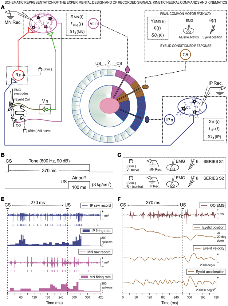
Figure 1. Schematic representation of the experimental design and of the recorded physiological signals, including the kinetic neural commands and kinematics of eyelid response. (A) Diagram illustrating the stimulating (Stim.) and recording (Rec.) sites, as well as the eyelid coil and electromyographic (EMG) electrodes implanted in the upper eyelid. Kinetic neuronal commands were computed from the firing activities of antidromically identified OO Mns located in the facial nucleus (VII n) and from neurons located in the ipsilateral cerebellar posterior IP nucleus (IP n). Abbreviations: R n, red nucleus; V n, trigeminal nucleus; CR, conditioned response; CS, conditioned stimulus; US, unconditioned stimulus. Here, the circle of colors is a diagram illustrating the idea of the conversion of a conventional data distribution to an angular distribution in order to study the corresponding time-dispersion patterns. (B) For classical conditioning of eyelid responses we used a delay paradigm consisting of a tone as a conditioned stimulus (CS). The CS started before, but co-terminated with, an air puff used as an unconditioned stimulus (US). Here the CS–US interval was 270 ms. (C) Diagrammatic representation of the experimental series, S1 for Mn and S2 for IP neuron recordings, both obtained in simultaneity with the EMG activities of the OO muscle and eyelid position recordings during classical eyeblink conditioning. (D,E) A set of recordings collected from the 10th conditioning session from two representative animals. Here are represented the kinetic [neural commands, in (D)] and the performance [kinematics, in (E)] of eyelid CR. (D) The action potentials (IP spikes) marked with blue plus signs correspond to the direct representation of the neuronal activity in the IP n (IP raw recordings) and its respective instantaneous frequency (IP firing rate). Action potentials (Mn spikes recorded from an OO Mn) are indicated with magenta plus signs. The direct representation of the neuronal activity in the facial nucleus (Mn raw recordings) and its corresponding instantaneous frequency (Mn firing rate) are shown. (E) These traces illustrate the EMG activity of the OO muscle (OO EMG), the direct recording of the eyelid position by the magnetic field search-coil technique, and the estimated eyelid velocity and acceleration curves. For each of the physiological signals represented, the magnitude and the respective unit of measurement are indicated.

Four of the animals were prepared for the chronic recording of antidromically identified facial Mns projecting to the OO muscle. For this, two stainless steel hook electrodes were implanted on the zygomatic subdivision of the left facial nerve, 1–2 mm posterior to the external canthus. The other four animals were prepared for the chronic recording of antidromically identified left posterior IPns. In this case, a bipolar stimulating electrode, made of 200 μm enamel-coated silver wire, was implanted in the magnocellular division of the right (contralateral) red nucleus following stereotaxic coordinates (Berman, 1968). A recording window (5 mm × 5 mm) was opened in the occipital bone of all of the animals to allow access to the facial or the IP nuclei. The dura mater was removed, and an acrylic chamber was constructed around the window. The cerebellar surface was protected with a piece of silicone sheet and sterile gauze, and hermetically closed using a plastic cap. Finally, animals were provided with a head-holding system for stability and proper references of coil and recording systems. All the implanted electrodes were soldered to a socket fixed to the holding system. A detailed description of this chronic preparation can be found elsewhere (Trigo et al., 1999; Gruart et al., 2000a; Jiménez-Díaz et al., 2004; Sánchez-Campusano et al., 2007).

Recording and Stimulation Procedures

Eyelid movements were recorded with the magnetic field search-coil technique (Gruart et al., 1995). The gain of the recording system was set at 1 V = 10°. The EMG activity of the OO muscle was recorded with differential amplifiers at a bandwidth of 0.1 Hz to 10 kHz. Action potentials were recorded in facial and IP nuclei with glass micropipettes filled with 2 M NaCl (3–5 MΩ resistance) using a NEX-1 preamplifier (Biomedical Engineering Co., Thornwood, NY, USA). For the antidromic activation of recorded neurons, we used single or double (interval of 1–2 ms) cathodal square pulses (50 μs in duration) with current intensities <300 μA. Only antidromically identified OO Mns and IPns were stored and analyzed in this study (Figure 1D). Site location and identification procedures have been described in detail for facial Mns (Trigo et al., 1999) and posterior IPns (Gruart et al., 2000a; Jiménez-Díaz et al., 2004; Sánchez-Campusano et al., 2007).

Classical Eyeblink Conditioning

Classical eyeblink conditioning was achieved by the use of a delay conditioning paradigm (Figure 1B). A tone (370 ms, 600 Hz, 90 dB) was used as CS. The tone was followed 270 ms from its onset by an air puff (100 ms, 3 kg/cm²) directed at the left cornea as a US. Thus, the tone and the air puff terminated simultaneously. Tones were applied from a loudspeaker located 80 cm below the animal’s head. Air puffs were applied through the opening of a plastic pipette (3 mm in diameter) located 1 cm away from the left cornea.

Each animal followed a sequence of two habituation, 10 conditioning, and three extinction sessions. A conditioning session consisted of 12 blocks separated by a variable (5 ± 1 min) interval. Each block consisted of 10 trials separated by intervals of 30 ± 10 s. Within each block, the CS was presented alone during the first trial – i.e., it was not followed by the US. A complete conditioning session lasted for ≈2 h. The CS was presented alone during habituation and extinction sessions for the same number of blocks per session and trials per block and with similar random inter-block and inter-trial distributions (Gruart et al., 1995).

Histology

At the end of the recording sessions, animals were deeply re-anesthetized (50 mg/kg sodium pentobarbital, i.p.). Electrolytic marks were placed in selected recording sites with a tungsten electrode (1 mA for 30 s). Animals were perfused transcardially with saline and phosphate-buffered formalin. Serial sections (50 μm) including the cerebellum and the brainstem were mounted on glass slides and stained with toluidine blue or cresyl violet, for confirmation of the recording sites (Gruart et al., 2000a; Jiménez-Díaz et al., 2004).

Data Collection and Multi-Parametric Statistical Analysis

The neuronal activity recorded in facial and cerebellar-IP nuclei, the EMG of the OO muscle, the eyelid position, and rectangular pulses corresponding to CS and US presentations, were stored digitally on a computer, using an analog–digital converter (CED 1401 Plus; Ceta Electronic Design, Cambridge, UK). Commercial computer programs (Spike 2 and SIGAVG; Ceta Electronic Design) were employed for acquisition and on-line conventional analyses. The multivariate off-line analyses of electrophysiological signals (including the analysis for the linear and non-linear correlation coefficients, the time delays, and the causality indices), the analytical procedures (including spike detection, multi-parametric cluster technique, circular time-dispersion method, and the fast Fourier transform), and the quantification and representation programs used for data illustrated in the main text, were developed by one of us (Raudel Sánchez-Campusano) with the help of MATLAB routines (The MathWorks, Natick, MA, USA). Only data from successful animals (i.e., those that allowed a complete study with an appropriate functioning of both recording and stimulating systems) were computed and analyzed.

The raw activities recorded from OO Mns and IPns were computed and quantified. The quantification algorithm also took into account the identification of the activity’s standard waveform and the classification of probability patterns of spikes in time and frequency domains (Jarvis and Mitra, 2001; Brown et al., 2004; Sánchez-Campusano et al., 2007), and in the phase space (Aksenova et al., 2003). Since raw neuronal recordings usually contain overlapping spikes, we selected the following analytical procedure. Using a spike-sorting method, overlapping spikes within an interval of 1 ms were regarded as a single spike (according to the absolute refractory period) and overlapping spikes within an interval of 1–3 ms were regarded as spikes of different classes due to the interspike interval (i.e., the relative refractory period of the neuron) criterion in spike detection. The cluster tools enabled us to determine the numbers of cells, classes, and spikes and their centers by measuring the distances between their trajectories in phase space (Porras-García et al., 2010). Spike phase space reconstruction was implemented using the time delay technique (Chan et al., 2008), and the reconstructed spike waveform (an ideal and undisturbed spike that can be used as a template for the sorting method) preserves essential characteristics and the major phase space trajectory of the original spike. Finally, the instantaneous firing rate was calculated as the inverse of the interspike intervals. Velocity and acceleration profiles were computed digitally as the first and second derivatives of eyelid position records after low-pass filtering of the data (−3 dB cutoff at 50 Hz and zero gain at ≈100 Hz; Domingo et al., 1997; Sánchez-Campusano et al., 2007).

Maximum eyelid displacements during CRs were determined in the CS–US interval, and the function corresponding to the collected data (frequency sample at 1000 Hz) in the CS–US interval was adjusted by a simple regression method. This method enabled fixing the trend for the points near the zero level of eyelid position and establishing a standardized algorithm for all the responses across all the blocks of trials. In this way, the typical randomness in the determination of CR onset was avoided. The onset of a CR was determined as the latency from CS presentation to the interception of the regression function with the maximum amplitude level (see Figure 2A). This method was applied across the successive conditioning sessions, always showing the appropriate precision and robustness.

FIGURE 2

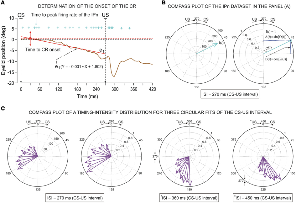
Figure 2. Determination of the onset of the eyelid conditioned response (CR) and some examples of the circular representation of the dataset distributions. (A) Illustration of an eyelid CR (eyelid position, in degrees) collected from a single trial during the 10th conditioning session. The onset of the CR (red arrow, from direct eyelid position recording using the magnetic search-coil technique) was determined as the latency (with respect to the conditioning stimulus (CS) presentation) corresponding to the interception (the red circle) of the regression function (see the red strength line and the equation e₁) with the maximum amplitude level (red dashed line). In this example, the time to CR onset is 30.0 ms. The action potentials (IPn spikes), marked with cyan plus signs, correspond to the direct representation of the firing activity in the IP neuron (311.1 spikes/s) collected during the same trial. The cyan arrow indicates the time to peak firing rate of the IPn (48.1 ms). (B) The circular representation of both parametric timing–intensity vector [48.1 ms, 311.1 spikes/s] and parametric timing unitary vectors [48.1 ms, 1 unit] of the IPn dataset represented as cyan plus signs in the (A). The blue dashed lines in (B) (see the second circle) serve to illustrate the sine and cosine components of the above angular data point. (C) The compass plots of parametric timing–intensity distribution of the Mn activity across the 10 conditioning sessions. Here, the dataset distribution is [time to peak firing rate of the OO Mns, Mn peak firing rate] (see the arrows for the actual values of the intensity components (in spike/s, see the first circle) and the normalized values of these (see the other three circle in this row) with respect to the maximum of the peak firing rates across conditioning sessions). The circles represent the three conversions of the CS–US interval to the angular plot (inter-stimulus interval, ISI = 270 ms; ^*ISI = 360 ms; ^*ISI = 450 ms) where ^*ISI denotes the simulated time conditions for studying the simulated dispersion patterns of the same dataset distribution.

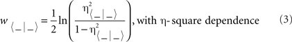
Computed results were processed for statistical analysis using the Statistics MATLAB Toolbox. As statistical inference procedures, both ANOVA (estimate of variance both within-groups and between-groups, on the basis of one dependent measure) and multivariate ANOVA (MANOVA, estimate of variance in multiple dependent parameters across groups) were used to assess the statistical significance of differences between groups. The corresponding statistical significance test (that is, the F_{[(m − 1), (m − 1) × (n − 1), (l − m)]} statistics and the resulting probability at the predetermined significance level P < 0.05) was performed, with sessions as repeated measures, coupled with contrast analysis when appropriate (Hair et al., 1998; Grafen and Hails, 2002). The orders m (number of groups), n (number of animals), and l (number of multivariate observations) were reported accompanying the F statistic values (Sánchez-Campusano et al., 2007, 2009). Wilk’s lambda criterion and its transformation to the χ²-distribution used in MATLAB were used to extract significant differences from MANOVA results (cluster analysis for cells-classes-spikes classification during the spike-sorting problem in the phase space, and hierarchical cluster free reconstruction during both actual and simulated causality conditions). The corresponding statistical significance tests (i.e., Student’s t-test and F statistic) were performed for the parameters of non-linear correlation analysis and causal inference method (see Linear and Non-linear Multivariate Analyses of Physiological Signals). Here, the hypothesis test is done by using the modified Fisher’s z-transformation (w) to associate each measured non-linear association index (η) with a corresponding w-transformation (see Non-linear Dynamic Associations Between Electrophysiological Recordings). For the circular statistics (Fisher, 1993; Jammalamadaka and SenGupta, 2001; Berens, 2009), we used both the Rayleigh and the Watson hypothesis tests to the von Mises distribution (Ψ, the circular analog of the normal distribution; see Circular Statistics to Analyze Time-Dispersion Patterns During Motor Learning for more details).

Linear and Non-Linear Multivariate Analyses of Physiological Signals

Multivariate analysis is extensively used with the aim of studying the relationship between simultaneously recorded signals or their equivalent time series. Multivariate time series tools [Non-linear dynamic association (see Non-linear Dynamic Associations Between Electrophysiological Recordings) and Time-dependent causality analysis (see Time-Dependent Causality Analysis Between Neuronal Firing Command and Learned Motor Response)] enabled us to determine the functional relatedness, asymmetry, time delay, direction in coupling, and causal inferences between physiological time series [i.e., neuronal activities generated in facial and cerebellar-IP nuclei (VII n or IP n, in Figures 1A,D), and learned motor responses (OO EMG activity or conditioned eyelid responses, in Figures 1A,E)] collected during classical conditioning sessions. In practice, we illustrated the use of multivariate analyses for the assessment of the strength (strong, moderate, or weak), type (linear or non-linear), directionality (unidirectional or bidirectional) and functional nature (feedforward or feedback relationships) of interdependencies between these physiological time series.

Non-linear dynamic associations between electrophysiological recordings

We used non-linear correlation analysis to investigate the following dynamic associations:

(1) Y_EMG(t) vs. X_MN(t); between the EMG activity of the OO muscle and the neuronal activity of facial nucleus (the OO Mns).

(2) Y_EMG(t) vs. X_IP(t); between the EMG activity of the OO muscle and the neuronal activity of IPns.

(3) Y_MN(t) vs. X_IP(t); between Mn and IPn activities.

The non-linear association index () between the electrophysiological time series X(t) and Y(t) was computed as,

with Ns being the number of samples of the signals, being the average of all amplitudes Y_k, and ℑ(X_j) being the piecewise approximation of the non-linear regression curve. In the above mathematical expression, Nb is the number of bins and B_j (with j = 1,…,Nb) are the different bins in the corresponding scatter representations. The measure of association in the opposite direction can be calculated analogously. In this formulation, the subscript _{〈Y | X〉} denotes the coupling from signal X(t) to the signal Y(t), _{〈X | Y〉} indicates the coupling in the opposite direction – that is, from signal Y(t) to the signal X(t), and _{〈− | −〉} denotes either of the two directions of coupling.

To assess the direction of coupling between the electrophysiological signals X(t) and Y(t), we used the following direction index (Wendling et al., 2001),

where and Δτ = τ_{〈Y | X〉} − τ_{〈X | Y〉}, with τ_{〈Y | X〉} (corresponding to η_{〈Y | X〉} and ) and τ_{〈X | Y〉} (corresponding to η_{〈X | Y〉} and ) being the time delays (i.e., the time shift τ_{〈− | −〉} for which is maximum) between signals.

Indeed, if X(t) causes Y(t), τ_{〈Y | X〉} will be positive and τ_{〈X | Y〉} will be negative, so that the difference Δτ will also be positive. In this case, the degree of asymmetry of the non-linear coupling Δη² will also be positive and therefore the direction index D = +1. These five previous conditions (τ_{〈Y | X〉} > 0; τ_{〈X | Y〉} < 0; Δτ > 0; Δη² > 0 and D = +1) should be satisfied simultaneously, to conclude that the relationship is of the type – that is, a unidirectional coupling between signals. In all the other combinations of conditions, the relationship will be false [i.e., a spurious unidirectional coupling, ].

If Y(t) causes X(t), τ_{〈Y | X〉} will be negative and τ_{〈X | Y〉} will be positive, so that the difference Δτ will also be negative. In this case, the degree of asymmetry of the non-linear coupling Δη² will also be negative, and as a consequence D = −1. These five previous conditions (τ_{〈Y | X〉} < 0; τ_{〈X | Y〉} > 0; Δτ < 0; Δη² < 0 and D = −1) should be satisfied simultaneously, to conclude that the relationship is of the type – that is, a unidirectional coupling between signals. In all the other combinations of conditions, the relationship will be false [i.e., a spurious unidirectional coupling, ].

If a feedback relationship between the signals X(t) and Y(t) is verified, then the time delays τ_{〈Y | X〉} and τ_{〈X | Y〉} will be positive, so that sgn(Δτ) ≠ sgn(Δη²) and therefore the direction index D = 0. The five previous conditions [(τ_{〈Y | X〉} > 0; τ_{〈X | Y〉} > 0; Δτ < 0; Δη² > 0 and D = 0) or (τ_{〈Y | X〉} > 0; τ_{〈X | Y〉} > 0; Δτ > 0; Δη² < 0 and D = 0)] should be satisfied simultaneously, to conclude that the relationship is of the type – that is, a bidirectional coupling or a feedback relationship between signals. If the signal Y(t) can be explained by the preceding signal X(t) better than vice versa, then in the contrary case . In all the other combinations of conditions, the relationship will be false [i.e., a spurious bidirectional coupling, ].

The statistical significance tests (i.e., Student’s t-test and F statistic) were performed for the parameters of non-linear correlation analysis (association indices and time delays). The hypothesis test was done by using the modified Fisher’s w-transformation (w_{〈− | −〉}) to associate each measured non-linear association index (η_{〈− | −〉}) with a corresponding w_{〈− | −〉} function,

For more details about linear and non-linear piecewise approximations of the regression curves, and statistical “multiple comparison” analyses, the reader may refer to Sánchez-Campusano et al. (2009, 2010) and Porras-García et al. (2010).

Time-dependent causality analysis between neuronal firing command and learned motor response

We investigated the dynamic regression models and causal inferences between neuronal firing function [SI_t: S1_t (MN), with f_MN(t) for facial Mn or S2_t (IP) with f_IP(t) for IPn instantaneous firing frequencies] and learned motor response [S0_t (θ), with θ(t) for eyelid positions during conditioned eyeblink responses] using the time-dependent causality analysis as a particular case of the transfer function models (TFM), a model frequently used to measure the functional interdependence between time series (Box and Jenkins, 1976; Granger, 1980; Nolte et al., 2008).

Relationships between Ns physiological time series [corresponding to instantaneous frequencies f_MN(t) and f_IP(t), and conditioned eyelid responses θ(t)] can be represented by transfer function models of the form

in which

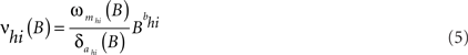
are the impulsive responses or transfer functions of the models. B is the back-shift operator such that BSI_t = SI_{t − 1}, and h = 1, 2, …, Ns. The moving average and autoregressive operators are also polynomials in B with orders m and a, respectively. The parameters b_hi are non-negative integers representing certain periods of delay in the transmission of the effects between the input SI_it and output S0_ht time series. The structure of the processes of inertia or uncertainties can be represented by the univariate operators (with orders p and q) in the stochastic difference equations of the form , where n_ht are Ns independent Gaussian white-noise processes with variances ρ_h and zero means (Tiao and Box, 1981).

Transfer function models of this form assume that the time series, when suitably arranged, possess a triangular relationship (Geweke, 1982; Harvey, 1994), implying for example that S2_t depends only on its own past (i.e., the Granger causality indices are such that G_{0 → 2} ≈ 0 and G_{1 → 2} ≈ 0); S1_t depends on its own past and on the present and past of S2_t (i.e., G_{1 → 2} = 0 and G_{2 → 1} > 0, for unidirectional coupling); S0_t depends on its own past and on the present and past of S1_t and S2_t (i.e., G_{0 → 1} = 0, G_{1 → 0} > 0, and G_{0 → 2} = 0, G_{2 → 0} > 0, respectively); and so on. If S1_t depends on its own past and on the present and past of S2_t, and S2_t depends on its own past and on the present and past of S1_t, then we must have a model that allows for this feedback (i.e., high and significant values of the causality indices in both senses G_{2 → 1} > 0 and G_{1 → 2} > 0, indicating bidirectional coupling). The normal (G_{1 → 0}) and normalized () Granger and Granger–Sargent () causality indices were calculated as

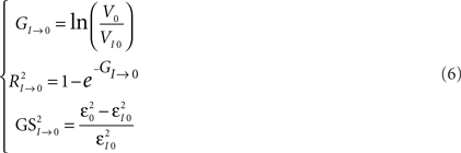
where V₀ and V₁₀ are the variances of the prediction errors and and the mean squared errors for both univariate and bivariate models (Kaminski and Liang, 2005). For more details about the theoretical formulation of these transfer function models and the above time-dependent Granger causality indices (Eq. 6), the reader may refer to Sánchez-Campusano et al. (2009).

Circular Statistics to Analyze Time-Dispersion Patterns during Motor Learning

This section provides a brief introduction to circular statistics (for more details see Batschelet, 1981; Fisher, 1993; Jammalamadaka and SenGupta, 2001; Berens, 2009). The term “circular statistics” describes a set of techniques used to analyze and to model distributions of random variables that are cyclic in nature (Mardia, 1975; Mardia and Jupp, 1999). For example, angles or directions differing by an integer multiple of 360° or 2π radians are considered to be equivalent. These techniques have enjoyed popularity in a number of areas where exploration, modeling, and testing hypotheses of directional information have played a role. Surprisingly, most work involving circular statistics has concentrated on directional data as described above, although the timing dataset such as the time of day, phase of the moon, or day of the year are also cyclic in nature. Circadian rhythms (or circadian timing) are most recognizable in nature but interval (in a wide seconds-to-minutes-to-hours range) and millisecond timing (sub-second range) also guide fundamental animal behaviors (Buhusi and Meck, 2005) that exhibit different periodicity and precision in various timing tasks. Therefore, timing across different timescales (sub-second range, seconds-to-minutes-to-hours range, and days-to-weeks range) may be also fitted to an angular scale.

In practical terms, circular quantification and compass representation do not require a cyclic or periodic condition (Batschelet, 1981). A compass plot is a two-dimensional polar plot with position vectors from the origin. While a compass plot can be drawn for arbitrary values it is useful to associate the plot with a polar trajectory definition. In fact, an appropriate time–angular correspondence was sufficient. The circular technique displays a compass plot having d arrows, where d is the number of elements in each one of the mean data T(i) (parametric timing or time delay) or I(i) (intensity or strength). The location of the base of each arrow is the origin. The location of the tip of each arrow is a point relative to the base and determined by the ith-observation [T(i), I(i)] where i = 1,…, d. In our application of circular distribution, the index d is the number of days (sessions) along the conditioning, or the number of blocks of the same session, or the total number of trials for all of the blocks of the same session, or the number of trials of the same block.

To convert parametric timing/time delay data T(i) in milliseconds to angles in degrees we assumed a direct interdependence determined by Eq. 7 at the intra-trail domain. Thus, the time dataset can be converted to a common angular scale in radians by the following equation:

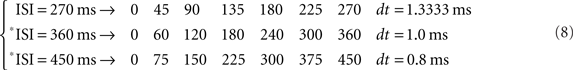
where Θ(i) and T(i) are the representations of the data in degrees and timescale, respectively, and Ω(i) is its angular representation in radians. k_Θ and k_T are the total numbers of steps on the scales used to measure Θ(i) and T(i). For example, if we have T(i) representing milliseconds from 0 ms (i.e., the CS onset instant) to 360 ms (i.e., 10 ms prior to the end of the US), then k_T = 360 steps of 1 ms – i.e., the simplest correspondence between time (in milliseconds) and angle (in degrees). However, we are interested in fitting the duration of the ISI to the circle according to our delay paradigm (see Figure 2B), where the actual duration of the ISI was 270 ms. Therefore, the total number of steps is k_T = 270 (i.e., 270 steps of 1.3333 ms, approximately). Note that this simple fitting to the circle is always possible for the different durations of the ^*ISI (the simulated time conditions for the different durations of the CS–US interval). In the array Eq. 8, we summarized the values for two simple conversions to the circle (see Figure 2C): (1) for ISI = 270 ms (i.e., less of a conventional cycle, 270 steps of 1.3333 ms), and (2) for ^*ISI = 450 ms (i.e., for more of a conventional cycle, 450 steps of 0.8 ms) in relation to the values of the conventional circle.

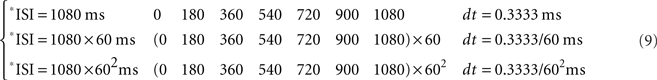
This strategy of transformation of the CS–US interval to the circle is easy to apply for ^*ISI ranging from sub-second range (millisecond timing) to seconds-to-minutes-to-hours range (interval timing); for example: ^*ISI of 1 s and 80 ms (1080 ms, i.e., 1080 steps of 0.3333 ms); ^*ISI of 1 min-4 s and 800 ms (1080 × 60 = 64800 ms, i.e., 1080 × 60 steps of 0.3333/60 ms); and ^*ISI of 1 h-4 min and 48 s (1080 × 60² = 3888000 ms, i.e., 1080 × 60² steps of 0.3333/60² ms), according to the following array:

Note that the relationship between the number of steps (i.e., the duration of the CS–US interval) and the time of sampling (dt) could be adapted in function of the temporal resolution of the data distribution. For example, if we have T(i) ranging from seconds to 1 min, then k_T = 60 steps of 1 s, and the time window (e.g., of the ISI) of 1 min is fitted to the circle according to the Eq. 7; for T(i) ranging from minutes to 1 h, k_T = 60 steps of 1 min, and the time window of 1 h is fitted to the circle; for T(i) ranging from hours to 1 day, k_T = 24 steps of 1 h, and the time window of 1 day is fitted to the circle; and finally, for T(i) ranging from days to 1 week, k_T = 7 steps of 1 day, and the time window of 1 week is fitted to the angular distribution also according to the Eq. 7.

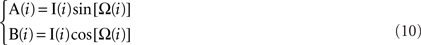
The parametric timing–intensity (or time delay–strength) distributions [T(i), I(i)] with i = 1,…, d, were represented as points on the circumference of a unitary circle – i.e., I(i) = 1 for all of the intensity/strength values, in the two-dimensional space. This is illustrated in Figure 2B, where a data point marked by a cyan circle lies on the unitary circumference. As indicated for the blue point in Figure 2B, the A(i)-coordinate of a point corresponds to the sine of the angle Ω(i) and the B(i)-coordinate to the cosine,

and the components of vectors [A(i), B(i)] were averaged as

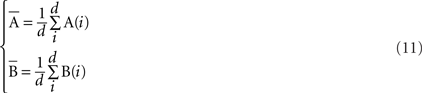
Thus, a more appropriate circular mean (in the circular statistics sense), denoted by in radians, was defined as

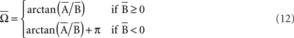
and the circular mean of the temporal distributions of the responses was

If all the angular measurements are represented as points on a circle, then a relatively simple geometrical interpretation of the circular mean may be shown, where the coordinates determine the centroid – i.e., the geometric center of the represented points. Thus, data sets (in radians or degrees) with a greater degree of circular spread (or dispersion index) have centroids closer to the center of the circle. Finally, the dispersion index σs was calculated as

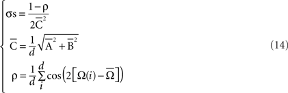
Note that is the radius of the circumference that describes the centroid with respect to the origin, and that higher values of are associated with less spread in the data. However, the dispersion index σs is in some respects more akin to the non-circular measurement of SD, as it has no upper bound, and larger values of ρs correspond to greater degrees of spread. In Eq. 14, ρ is a measurement of circular kurtosis, and a value close to one is indicative of a strongly peaked distribution (Berens, 2009). The circular variance V_C and standard angular deviation S_C are closely related to the mean resultant radius . These circular measurements are defined as and The circular variance is bounded in the interval [0,1] and the standard angular deviation lies in the interval [] (Berens, 2009). Furthermore, notice that the variable ρ is an implicit function of k_T [i.e., the total number of steps on the timescale used to measure T(i)]:

The mathematical expression (15) indicates that the time-dispersion index (σ) and time–intensity dispersion index (σs) are functions of the total number of steps (k_T) on the timescale, and therefore of the ISI (or CS–US interval), at least in this circular statistical sense.

The same applies to the von Mises distribution (Ψ, the circular analog of the normal distribution) where the probability densities of are given by

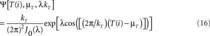
where μ_T is the mean value of T(i) (i.e., the maximum likelihood estimator of μ_T is ), λ is the concentration parameter related to the circular spread, and J₀(λ) is a normalization constant to ensure that the probability density integrates to one. In addition to this, it is also possible to carry out two hypothesis tests (Jammalamadaka and SenGupta, 2001):

(1) Rayleigh hypothesis test: explores whether T(i) has a uniform distribution – i.e., the concentration parameter related to the circular spread λ = 0;

(2) Watson hypothesis test: explores whether T(i) has the same mean for p distributions – i.e., μ1_T = μ2_T = … = μ p_T.

Finally, we assumed two circumstances for the dispersion analyses:

(1) Inter-stimulus interval of fixed duration (e.g., 270 ms) and different parametric timing–intensity (or time delay–strength) data distributions of the type [T(i), I(i)]. For example: (the time to IPn peak firing rate, the amplitude of this peak), or (the time to CR onset, the percentage of the CR), or other time delay–strength distributions. In this circumstance, we determined the dispersion patterns for the different time–intensity distributions of the datasets [i.e., (timing parameters, kinetic neural commands, and kinematic parameters), and (time delays, correlation code parameters)].

(2) Inter-stimulus interval of different durations as the simulated time conditions (e.g., 360 ms; 450 ms; 1080 ms, 1080 ms × 60 ms, 1080 ms × 60² ms; see the Eqs. 8 and 9) for the same time–intensity (or time delay–strength) data distribution [T(i), I(i)]. This circumstance is not interval timing (seconds-to-minutes-to-hours range), but it allowed us to show how the timing tasks can be treated mathematically using the circular distribution, an approach that we are already exploring in the different temporal domains (the inter-trials dispersion of the same block, the inter-blocks dispersion of the same session, and the inter-sessions dispersion along the process). Thus, we calculated the dispersion patterns of the same dataset distribution as a function of the ISI duration.

Consequently, for two time–intensity distributions [T1(i), I1(i)] and [T2(i), I2(i)] in a fixed CS–US interval (circumstance 1) or for two different ISI (ISI1 and ISI2) of the same time–intensity distribution (circumstance 2), it is always possible to calculate the time–intensity dispersion indices σs1 and σs2, respectively, and therefore, the fraction of dispersion indices is defined as

Notice in (17) the following relationships between the indices , ρ, and σs,

If (the radii that describe the centroids with respect to the origin), then ρ2 > ρ1, and therefore σs2 < σs1.

If (the radii that describe the centroids with respect to the origin), then ρ1 > ρ2, and therefore σs1 < σs2.

In this paper, we calculated the following dispersion indices in the different temporal domains (the inter-trials dispersion of the same block, the inter-blocks dispersion of the same session, and the inter-sessions dispersion along the process).

(a) σ_MN and σs_MN, for the timing and timing–intensity distributions from the firing activity of the Mns (e.g., see Figure 2C).

(b) σ_CR and σs_CR, for the timing and timing–intensity distributions from the eyelid CRs.

(c) σ_IP and σs_IP, for the timing and timing–intensity distributions from the firing activity of the IPn.

(d) σ0 and σs0, for the time delay and time delay–strength distributions from τ0_{〈f IP | θ〉} and r_{max〈f IP | θ〉}

(e) σ1 and σs1, for the time delay and time delay–strength distributions from τ1_{〈EMG | MN〉} and η1_{max 〈EMG | MN〉}

(f) σ2 and σs2, for the time delay and time delay–strength distributions from τ2_{〈MN | EMG〉} and η2_{max 〈MN | EMG〉}

(g) σ3 and σs3, for the time delay and time delay–strength distributions from τ3_{〈EMG | IP〉} and η3_{max 〈EMG | IP〉}

(h) σ4 and σs4, for the time delay and time delay–strength distributions from τ4_{〈IP | EMG〉} and η4_{max 〈IP | EMG〉}

(i) σ5 and σs5, for the time delay and time delay–strength distributions from τ5_{〈MN | IP〉} and η5_{max 〈MN | IP〉}

(j) σ6 and σs6, for the time delay and time delay–strength distributions from τ6_{〈IP | MN〉} and η6_{max 〈IP | MN〉}

Results

We recorded a total of 105 posterior IPns, classified as type A (Figures 1A,D). Type A neurons increase their firing in the time interval between conditioned (CS) and unconditioned (US) stimulus presentations across successive conditioning sessions (Gruart et al., 2000a; Sánchez-Campusano et al., 2007). In addition, we recorded 102 antidromically identified OO MNs (Figures 1A,D). Characteristically, OO Mns encode eyelid position during CRs (Trigo et al., 1999; Sánchez-Campusano et al., 2009). The two pools of neurons were recorded in separate experiments during classical eyelid conditioning (Figures 1A,C) using a delay paradigm (Figures 1A,B, see Materials and Methods). The present study was centered on the analysis of data collected in CS–US intervals across the successive sessions during the motor learning process. A more detailed description of OO Mn and IPn firing peculiarities during classical eyeblink conditioning can be found elsewhere (Trigo et al., 1999; Gruart et al., 2000a; Sánchez-Campusano et al., 2007, 2009, 2010).

Multiple Parametric Evolutions of the Timing, Kinetic Neural Commands, and Kinematic Parameters during Classical Conditioning of Eyelid Responses

A representation of the different parameters collected across conditioning sessions is illustrated in Figure 3. In Figure 3A, we show the timing parameters and in Figure 3B the kinetic (neural commands) and kinematic (performance of learned motor response) parameters computed here, presenting a coherent timing–intensity association between them (e.g., parameters 1 and 6; 2 and 7; 3 and 8; 4 and 9; 5 and either 10 or 11). In Figure 3A, the mean values of the relative refractory period of OO Mns (parameter 1) in the CS–US interval decreases across conditioning sessions [one-way ANOVA F-test, F_{(14, 70, 132)} = 206.20, P < 0.01], and the latency of their maximum instantaneous frequency with respect to CS presentation [parameter 2, F_{(14, 70, 132)} = 53.19, P < 0.01] also decreases. The similar inverted evolution (from long to short periods or latencies) was obtained for the mean values of the relative refractory period of the IPns [parameter 3, F_{(14, 70, 132)} = 126.44, P < 0.01] and for the latency (with respect to CS onset) of their maximum instantaneous frequency in the CS–US interval [parameter 4, F_{(14, 70, 132)} = 93.87, P < 0.01] across conditioning sessions. Finally, the parameter 5 (mean values of the latency between the CS onset and the start of the CR, see Figure 2A) also decreases with significant statistical differences [F_{(14, 70, 132)} = 123.50, P < 0.01] along the conditioning process.

FIGURE 3

Figure 3. A representation of multi-parametric evolution of timing, kinetic and kinematic parameters collected across habituation, conditioning, and extinction sessions. The color code indicates the corresponding conditioning session (from C01 to C10), each set of colored bars corresponds to the evolution of a given parameter (numbered from 1 to 11), and each colored bar indicates the mean parametric value resulting from averaging the trials of the same session, a procedure applied for each of the sessions. (A) The multiple parametric evolution of the timing parameters in the CS–US interval: parameters 1 and 3 (relative refractory period – i.e., the minimum interspike interval, in s), 2 and 4 (latency of the mean value of maximum instantaneous frequency with respect to CS presentation, in ms), and 5 (latency between the CS and the onset of the CR, in ms). (B) The multiple parametric evolution of the kinetic and kinematic parameters across sessions: parameters 6 and 8 (total number of spikes in the CS–US interval), 7 and 9 (mean peak firing rate, in spikes/s), and 10 (eyelid position amplitude at US presentation compared with the amplitude at the start of the CR, in degrees). The timing (parameters 1–4) and kinetic (parameters 6–9) parameters were calculated for both OO Mns (Mn, parameters 1, 2, 6, and 7) and IP neurons (parameters 3, 4, 8, and 9). The parameters 5, 10, and 11 characterize the proper timing and performance (kinematics) of learned eyelid responses. (C) The typical learning curve (evolution of the parameter 11) using this classical conditioning paradigm. For this timing–kinetic–kinematic multi-parametric representation, each parameter has been normalized in accordance with its maximum value across conditioning.

As illustrated in Figure 3B, the kinetic neural commands and kinematic parameters presented in general an opposite evolution (from low to high values) across conditioning sessions with respect to the evolution of the timing parameters shown in Figure 3A. For example, the total number of spikes generated by OO Mns (parameter 6) during the CS–US interval increases across conditioning sessions [one-way ANOVA F-test, F_{(14, 70, 132)} = 187.12, P < 0.01] and their mean peak firing rate (parameter 7) also increases [F_{(14, 70, 132)} = 207.31, P < 0.01], indicating that this dorsolateral portion of the facial nucleus (the site where OO Mns are located) was involved as the neural element driving (kinetic neural command) the eyelid CRs. Interestingly, the mean number of spikes (parameter 8) generated by IPns in the CS–US interval did not change significantly [F_{(14, 70, 132)} = 1.63, P > 0.05] across conditioning. In contrast, the mean peak firing rate of IPns [parameter 9, F_{(14, 70, 132)} = 143.86, P < 0.01] increased across conditioning sessions and decreased progressively during the three extinction sessions. These contrasting evolutions suggest that the increase in IP neuronal firing rate after CS presentation represented a reorganization (rather than a net increase) of their mean spontaneous firing. Finally, parameter 10 in Figure 3B corresponds to the peak amplitude of the evoked CR. Note that this parameter also increased steadily across conditioning sessions and decreased progressively during the three extinction sessions [F_{(14, 70, 132)} = 251.27, P < 0.01].

The evolution of these intensity/amplitude parameters (6, 7, 9, and 10 in Figure 3B) across conditioning was analogous to that verified for the parameter 11 [F_{(14, 70, 132)} = 129.40, P < 0.01] – i.e., the percentage of CRs across conditioning (Figure 3C) – and to the one observed previously in typical learning curves using the same classical conditioning paradigm (Domínguez-del-Toro et al., 2004; Gruart, et al., 1995; Sánchez-Campusano et al., 2007, 2009, 2010; Porras-García et al., 2010). Finally, note that in Figure 3, the parameters were normalized in accordance with their maximum values across conditioning. Thus, the maximum values of the mean latencies of the maximum instantaneous frequencies were 259.14 ms (parameter 2, session H01) and 93.06 ms (parameter 4, session H01) for Mns and IPns, respectively; the maximum values of mean number of spikes generated in the CS–US interval (parameters 6 and 8) were 9.83 spikes (in session C09) and 15.38 spikes (in session C02) for Mns and IPns, respectively; and the maximum values of mean peak of the firing rate were 158.27 spikes/s (parameter 7, session C09) and 322.60 spike/s (parameter 9, session C10) for both Mns and IPns, respectively.

The Evolution of the Correlation Code Parameters and Falling Correlation Property of the Interpositus Nucleus Neurons

In the previous sections, we have presented results relating to the acquisition and representation of the physiological multi-parametric data (Figure 3) collected across conditioning sessions and the level of expression of eyelid CRs. These results (quantitative multi-parametric analyses and the learning curve) were necessary but insufficient for a precise dynamic description of the conditioning process. In this section, we use an analytical approach (the non-linear multivariate analysis of electrophysiological recordings) to understand the functional correlation code and the directional coupling mechanisms (see Non-linear Dynamic Associations Between Electrophysiological Recordings) between the EMG activity of the OO muscle and crude recordings of both facial and IP nuclei, and between the two neuronal recordings (Mn and IPn activities) during the classical conditioning of eyelid responses.

In a previous study from our group (Sánchez-Campusano et al., 2009) we showed the non-linear association analyses at the asymptotic level of acquisition (i.e., the 10th conditioning session) of this associative learning test (details regarding the theoretical formulation of this dynamic association method for the electrophysiological recordings can be found in Sánchez-Campusano et al., 2009, 2010 and in Porras-García et al., 2010). In the present paper, we carry out the exhaustive analyses of dynamic associations between the recordings during all the conditioning sessions (see Figure 4A). The degree of association between the EMG activity of the OO muscle [Y_EMG(t)] and crude recordings of neuronal responses [X_NR(t)] collected from facial [X_MN(t)] and IP [X_IP(t)] neurons was obtained by computing the non-linear association index η_{〈− | −〉} as a function of a time shift τ_{〈− | −〉} between these muscular and neuronal electrophysiological recordings. The association between the two neuronal activities was also analyzed [Y_MN(t) vs. X_IP(t) and vice versa].

FIGURE 4

Figure 4. The trend in the evolution of the correlation code parameters (linear and non-linear correlation coefficients and the asymmetry information) and the inverse dependence of this on the evolution of the peak firing rate of IP neurons across conditioning sessions (from C01 to C10). (A) The color code indicates the four dynamic associations [magenta, for Mn raw activity vs. OO EMG recording (OO EMG); blue, for IP neuron raw activity vs. OO EMG; green, for IPn vs. Mn raw recordings; and red, for IP neuron instantaneous frequency f_IP(t) vs. the eyelid position θ(t) response] for this analysis. Each colored triangle pointing toward the right corresponds to the mean value of maximum non-linear association index in the preferential direction of coupling [η1_{max 〈EMG|MN〉}, η3_{max 〈EMG | IP〉}, and η5_{max 〈MN | IP〉}] and each colored triangle pointing toward the left indicates the mean values of maximum non-linear association index in the opposite direction [η2_{max 〈MN | EMG〉}, η4_{max 〈IP | EMG〉}, and η6_{max 〈IP | MN〉}, see the legend]. Each red triangle pointing up corresponds to the mean value of maximum linear correlation coefficient [r_{max〈f IP | θ〉}] calculated during a conditioning session. The colored lines represent the linear regression models for each set of maximum association indices across conditioning sessions. The three ranges of correlation coefficient values (high, middle, and low) are indicated. The magnitudes Δη12_max, Δη34_max and Δη56_max indicate the difference (asymmetry information) between the pairs of maximum association indices at the asymptotic level (the 10th session) of acquisition of this associative learning test. (B) The abscissa and the left ordinate illustrate the relationship between the peak firing rate of IP neurons (f_{IP max}) and the percentage of CRs (%CRs; brown squares; e1 regression line). The abscissa and the right ordinate illustrate the relationship between f_{IP max} and the correlation code (red triangles, r_{max〈f IP | θ〉} linear correlation coefficients, e2 regression line; blue and green triangles, η3_{max 〈EMG | IP〉}, …, η6_{max 〈IP | MN〉} non-linear association indices, e3, …, e6 regression lines). Note that both the level of expression of CRs (i.e., %CRs) and the evolution of f_{IP max} depend inversely on the evolution of strength (from strong to moderate, or from moderate to weak) of the dynamic associations (i.e., the linear and non-linear correlation coefficients) between the IP neuron (IPn) activity and either the Mn kinetic neural command or kinematic variable (eyelid position or OO EMG). In Table 1 are summarized the regression parameters for this figure.

The non-linear association functions corresponding to the trials taken from the same session were averaged, session by session and for each experimental subject. The present study was centered on the analysis of the data (correlation codes and time delays) collected at CS–US intervals across the 10 conditioning sessions (C01–C10). In Figure 4A, we represent the maximum values of non-linear association indices (η_max) and their evolution across training. The maximum indices between Mns activity and OO EMG recording remained high (η_max ≥ 0.75) across conditioning sessions. The magenta regression lines [for the evolution of the indices η1_{max 〈EMG | MN〉}and η2_{max 〈MN | EMG〉}] showed a strongly increasing trend (see the parameters of this trend analysis – i.e., the magnitudes and signs of the correlation coefficients R, the significances P, and the equations (slope and intercept) of the regression lines, in Table 1). Thus, motoneuronal activities correlate significantly [one-way ANOVA F-tests, F_{(9, 27, 98)} = 3.06, P < 0.01 for η1_{max 〈EMG | MN〉}; and F_{(9, 27, 98)} = 2.51, P < 0.01 for η2_{max 〈MN | EMG〉}] with the EMG activity of the OO muscle during the performance of conditioned eyelid responses in all the conditioning sessions. However, the increase in the mean peak firing rate of IPns (parameter 9 in Figure 3B), together with the decrease in its time of occurrence (parameter 4 in Figure 3A), always lagged the start of the CR (see Figure 2A) and caused a decrease in the non-linear association indices between IPn activity and eyelid CRs (determined by OO EMG activity) across conditioning (see Figure 4A). A standard analysis of the trends using linear regression models enabled us to determine the evolution of the η_max across training (in all of the regressions see the signs of R and the slope in Table 1). For example, the blue and green regression lines [for the evolution of the indices η3_{max 〈EMG | IP〉}, η4_{max 〈IP | EMG〉}, η5_{max 〈MN | IP〉}, and η6_{max 〈IP | MN〉}] showed clear negative slopes (see Table 1), and therefore a decrease (the negative signs of R) of correlation levels in accord with non-linear correlation analyses. In turn, the values of the maximum non-linear association indices were statistically significant across conditioning sessions [one-way ANOVA F-tests, F_{(9, 27, 98)} = 7.26, P < 0.01, for η3_{max 〈EMG | IP〉}; F_{(9, 27, 98)} = 11.02, P < 0.01, for η4_{max 〈IP | EMG〉}; F_{(9, 27, 98)} = 9.45, P < 0.01, for η5_{max 〈MN | IP〉}; F_{(9, 27, 98)} = 12.33, P < 0.01, for η6_{max 〈IP | MN〉}], although their values showed only a slight coupling (0.5 ≤ η_max < 0.8, i.e., the two signals were moderately related) between the neuronal activity recorded at the IP nucleus [X_IP(t)] and either the EMG activity of the OO muscle [Y_EMG(t)] or Mn neuronal recording [X_MN(t)] during the performance of the conditioned eyelid responses. In this particular case, the maximum values of mean association indices always lagged the zero reference point (i.e., the moment at which the conditioned eyelid response started, see red arrow in Figure 2A) in all the successive conditioning sessions.

TABLE 1

Table 1. The parameters of the linear regression analyses [the correlation coefficient (R), the significance level (P), and the linear equation parameters (slopes and intercepts)] for the Figures 4A,B.

Interestingly, for all the dynamic association analyses, the degree of asymmetry of the non-linear coupling between the pairs of electrophysiological recordings (IPn activity vs. either Mn or OO EMG recordings) was positive during all the conditioning sessions. Here we summarize the results for the information of asymmetry in the 10th conditioning session [ with , with Δη34_max = η3_max − η4_max ≈ 0.2010; , with Δη56_max = η5_max − η6_max ≈ 0.1340] (see Figure 4A in this paper, and Sánchez-Campusano et al., 2009 for details of the non-linear association curves and their maximum correlation values). Note that, for the coupling between Mns [X_MN(t)] and OO EMG [Y_EMG(t)] recordings, the values and Δη12_max [for the indices η1_{max〈EMG | MN〉}and η2_{max 〈MN | EMG〉}] across conditioning sessions indicate a decrease in the degree of asymmetry in coupling [e.g., a variation of 7.21% for Δη12_max, which diminishes from 0.1041 (in session C01) to 0.0320 (in session C10)]. In geometrical terms, the progressive convergence of the red regression lines (i.e., a progressive loss in the degree of asymmetry) and the proper gain in the strength (the non-linear association indices, see Figure 4A) of coupling along conditioning allowed us to conclude that at the asymptotic level of acquisition of this associative learning test (session C10), the recording Y_EMG(t) can be explained as a quasi-linear transformation of the Mns activity X_MN(t).

However, the degree of asymmetry increased across conditioning sessions for the other two dynamic associations [Y_EMG(t) vs. X_IP(t), a variation of 12.9% for Δη34_max, which increased from 0.0720 (in session C01) to 0.2010 (in session C10); and Y_MN(t) vs. X_IP(t), a variation of 12.45% for Δη56_max, which increased from 0.0095 (in session C01) to 0.1340 (in session C10)]. Thus, one signal [i.e., Y_EMG(t) or Y_MN(t)] can be explained as a transformation, possibly non-linear, of the other [i.e., X_IP(t)]. This gain in the degree of asymmetry (see in Figure 4A the increasing divergence between the blue (or green) pair of regression lines) and the verified loss in the strength of coupling (negative trends in the evolutions of the non-linear association indices) along conditioning demonstrated that a quasi-linear and unidirectional coupling between the recordings [X_IP(t) vs. Y_MN(t) or X_IP(t) vs. Y_EMG(t)] was very unlikely, at least in the statistical sense. Finally, we could verify the falling correlation property of the IP nucleus across the successive training sessions, using the linear correlation coefficient r_{max〈f IP | θ〉} [one-way ANOVA F-tests, F_{(9, 27, 98)} = 161.54, P < 0.01] between the firing rate of IPns f_IP(t) and the eyelid position response θ(t) (see the red triangles and red regression lines in Figure 4A).

Inverse Dependence between the Strength of Dynamic Associations and the Firing Rate of Interpositus Nucleus Neurons

In Section “Multiple Parametric Evolutions of the Timing, Kinetic Neural Commands, and Kinematic Parameters During Classical Conditioning of Eyelid Responses” and “The Evolution of the Correlation Code Parameters and Falling Correlation Property of the Interpositus Nucleus Neurons” we analyzed the multiple parametric evolutions of the kinetic neural commands (parameters 6, 7, 8, and 9 in Figure 3B) and kinematic parameters (parameters 10 and 11), as well as the trends in the evolution of the correlation code parameters [the linear and non-linear correlation coefficients in Figure 4B, r_{max〈f IP | θ〉}; η1_{max 〈EMG | MN〉}and η2_{max 〈MN | EMG〉}; η3_{max 〈EMG | IP〉} and η4_{max 〈IP | EMG〉}; η5_{max 〈MN | IP〉} and η6_{max 〈IP | MN〉}, respectively] across conditioning. In this section, we summarize the dependence between the strength of the dynamic associations (correlation coefficient values in Figure 4A) and both the evolution of the peak firing rate of the IPns (i.e., the maximum amplitude of the instantaneous frequency f_{IP max} in the CS–US interval, parameter 10 in Figure 3B) and the level of expression of conditioned eyeblink responses (i.e., the percentage of CRs, parameter 11 in Figure 3B) across this associative learning process.

In Figure 4B, note that the increase in the peak firing rate of IPns f_{IP max} (e1 regression line) together with the decrease in its time of occurrence (it always lagged the start of CRs), caused a decrease in the linear correlation coefficient (e2 regression line for r_{max〈f IP | θ〉}) across conditioning sessions. In turn, a similar decrease was observed for the maximum values of the non-linear association indices [see the regression lines, e3 for η3_{max 〈EMG | IP〉}; e4 for η4_{max 〈IP | EMG〉}; e5 for η5_{max 〈MN | IP〉}; and e6 for η6_{max 〈IP | MN〉}]. Thus, the evolution of the strength (strong, moderate, or weak) of the linear and non-linear dynamic associations (i.e., the coefficients r_max and η3_max, …, η6_max) depends inversely on the level of expression of conditioned eyeblink responses (i.e.,%CR) and of the evolution of f_{IP max} across learning. There is a significant increase (see R > 0, P < 0.01, and the positive sign of the slope of the regression line e1 in Figure 4B and Table 1) in the amplitude–intensity mutual evolution (f_{IP max} as a kinetic neural command and %CR as a measure of the performance of learned motor responses) and a significant decrease (see R < 0, P < 0.01, and the negative signs of the slopes of the regression lines e2, e3, e4, e5, and e6 in Figure 4B and Table 1) in the amplitude–strength mutual evolution (f_{IP max} and r_max, η3_max, η4_max, η5_max, and η6_max) across conditioning sessions.

Interactions between the Parametric Timing Information and the Time Delays in Coupling between the Electrophysiological Recordings

In previous sections, we showed the evolution of the parametric timing information (see the timing parameters in Figure 3A) collected across conditioning. Additionally, we used the so-called “time delay information” to express the temporal order in the cerebellar–Mns network. According to the dynamic association method (see non-linear dynamic associations between electrophysiological recordings), the shift for which the maximum of the non-linear association index η_{〈− | −〉} was reached provided an estimate of the time delay τ_{〈− | −〉} in coupling between the electrophysiological time series during this associative learning process. Thus, we were able to determine whether the maximum correlation (strong, moderate, or weak) between the recordings was before or after the zero reference point (i.e., the moment at which the CR started, Figure 2A).

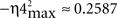
At the same time, a set of techniques referred to as circular statistics has been developed for the analysis of directional and orientational data. The unit of measurement for such data is angular (usually in either degrees or radians) and the circular distributions underlying the techniques are characterized by the proper time–degree correspondence. In this paper, we assert that such approaches can be easily adapted to analyze the different events in the 0- to 270-ms interval (the duration of ISI, i.e., the CS–US interval) during the performance of the CR – for example, the angle of 0 degrees is deemed as corresponding to a time of 0 ms – that is, the CS onset instant; and the angle of 270° is deemed as corresponding to the time of US presentation – that is, 270 ms after CS onset, according to our delay paradigm (see Figure 1B). In Figures 5A and 6A we show the circular distributions of both parametric timing–intensity and time delay–strength distributions across conditioning sessions, using a compass plot to analyze time–intensity dispersion patterns in this learning process.

In Figure 5, we selected as the timing components of the distributions the time to CR onset (see brown arrows) and the time to peak firing rate of the IPn (see cyan arrows), and the corresponding intensity components of the represented distributions were the percentage of CRs and the peak firing rate of the IPn, respectively (see Figures 5A,B). In many situations, the interpretation of the evolution of a physical magnitude lacks a proper complementation between the evolution of its intensities/amplitudes and the temporal dynamics of its variations. Thus, these timing–intensity associations enabled us to illustrate the simultaneous evolution of the timing and intensity components of these data distributions across conditioning sessions (see Figure 2C and the second row in Figure 5A). Notice the inverse interrelations between the percentage of CRs and the time to CR onset (arrows and histogram in brown), and between the peak firing rate of the IPn and their corresponding time of occurrence (arrows and histogram in cyan) across this associative learning test (Figures 5A,B). However, the time to peak firing rate of the IPn always lagged the beginning of the CR (see the cyan and brown circular sectors and histograms in Figure 5B).

FIGURE 5

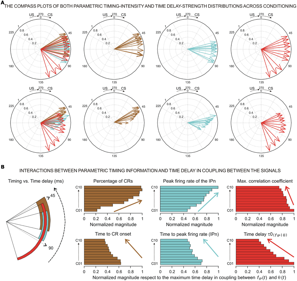
Figure 5. (A) The compass plots of both parametric timing–intensity and time delay–strength distributions across the 10 conditioning sessions. In this representation, the timing–intensity distributions (1) [time to CR onset, and percentage of CR], see brown arrows, and (2) [time to peak firing rate of IP neurons (IPn) peak firing rate], see cyan arrows, and the time delay–strength distributions (3) [time delay in coupling τ0_{〈f IP|θ〉}, maximum linear correlation coefficient r_{max〈f IP | θ〉}], see red arrows, were plotted using the circular approach for the inter-stimulus interval of 270 ms (CS–US interval). The 10 colored arrows (10 conditioning sessions, C01–C10) in each circle illustrate the circular dispersion of the angular datasets represented. The first row of circles corresponds to the representation of the time (timing and time delay) distributions on the unitary circle to explore the time-dispersion patterns of datasets (see the dispersion parameters in Table 2), and the second row of circles shows the time–intensity distributions in accordance with the actual intensity/strength components to investigate the time–intensity dispersion patterns across conditioning (see the dispersion parameters in Table 3). (B) Interactions between parametric timing information and time delay in coupling between the firing rate of the IPn neurons f_IP(t) and the eyelid position θ(t) response. The colored circular sectors illustrate the time-dispersion range of the data distributions represented in (A) (see Table 2). The colored histograms show the normalized mean values of intensity/strength components of the distributions and the normalized mean values of timing/time delay components with respect to the maximum time delay in coupling between f_IP(t) and θ(t) [i.e., the maximum values of τ0_{〈f IP | θ〉} across conditioning sessions].

In this paper, the circular statistics enabled us to determinate the index of dispersion, which measures the degree of spread for these physiological circular data (see Circular Statistics to Analyze Time-Dispersion Patterns During Motor Learning). Thus, the dispersion patterns could provide an appropriate means of estimating the contribution (time-intensity) of the different centers (in the cerebellar-IP/red-nucleus-Mns pathway) participating in the conditioning process. The left-hand circumferences in Figures 5A and 6A and the left-hand circular sectors in Figures 5B and 6B show the circular dispersions of the timing and time delay parameters. For example, in Figure 5A the mean values of the time to peak firing rate of the IPn across the conditioning sessions (cyan arrows) were less spread out than the mean values of either time to CR onset (brown arrows) or time delay τ0_{〈f IP | θ〉} in coupling between IPn instantaneous frequency and eyelid position response (red arrows). Interestingly, the time-dispersion range for the time delay τ0_{〈f IP | θ〉} showed a significant [one-way ANOVA F-tests, F_{(9, 27, 98)} = 223.54, P < 0.01] transition from larger to smaller values, than the time to peak firing rate of IPn across the sessions. Thus, to the beginning of the learning process the IPns encoded (from moderate to weak correlation) eyelid position response after reaching their maximum firing rate, but at the end of the process (i.e., at the asymptotic level of acquisition of this associative learning test) the IPns encoded (with barely significant correlation) eyelid kinematics before their peak firing rate (but always after the beginning of the CR).

FIGURE 6

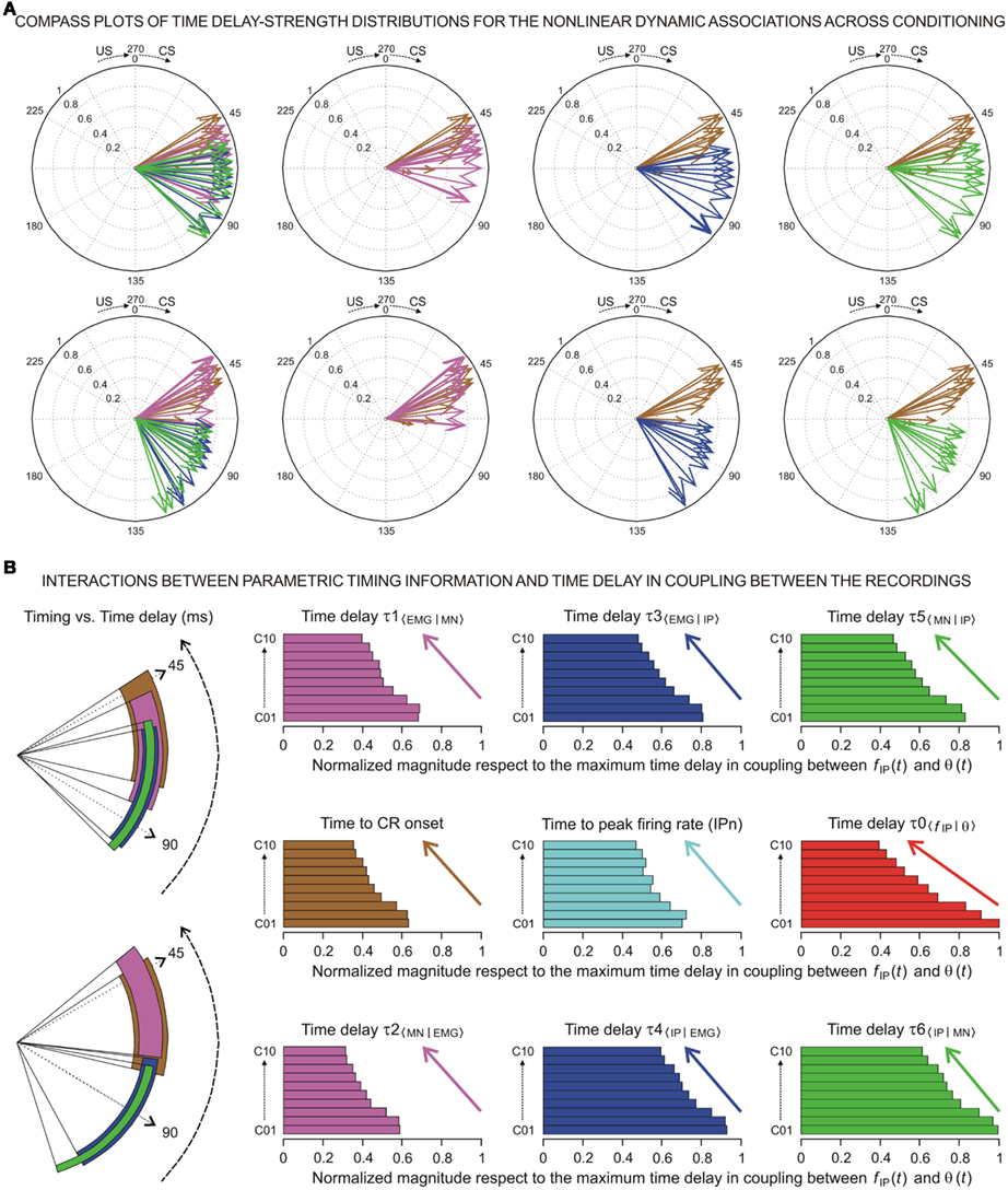
Figure 6. (A) The compass plots of time delay–strength distributions for the non-linear dynamic associations across the 10 conditioning sessions. In this representation, the time delay–strength distributions (1) [τ1_〈EMG|MN〉, η1_{max 〈EMG | MN〉}] and (2) [τ2_{〈MN | EMG〉}, η2_{max 〈MN | EMG〉}], see magenta arrows, (3) [τ3_{〈EMG | IP〉}, η3_{max 〈EMG | IP〉}] and (4) [τ4_{〈IP | EMG〉}, η4_{max 〈IP | EMG〉}], see blue arrows, and (5) [τ5_{〈MN | IP〉}, η5_{max 〈MN | IP〉}] and (6) [τ6_{〈IP | MN〉}, η6_{max 〈IP | MN〉}], see green arrows, were plotted using the circular statistics method for the inter-stimulus interval of 270 ms (CS–US interval). The 10 colored arrows (10 conditioning sessions, C01–C10) in each circle illustrate the circular dispersion of the angular datasets represented. The two rows of circles show the time delay–strength distributions to explore the time–strength dispersion patterns across conditioning (see the dispersion parameters in Table 3). (B) Interactions between parametric timing information and time delays in coupling between the recordings. The colored circular sectors illustrate the time-dispersion range of the data distributions represented in (A) (see the dispersion parameters Table 2).The colored histograms show the normalized mean values of timing/time delay components of the distributions with respect to the maximum time delay in coupling between f_IP(t) and θ(t) [i.e., the maximum values of τ0_{〈f IP | θ〉} across conditioning sessions].

In geometric terms, the centroid (in a two-dimensional space with a fixed intensity component and variable timing component) of the cyan circular sector (corresponding to the time to peak firing rate of the IPn in Figure 5B) was much further away from the center of the circumference than the centroid of the red circular sector [corresponding to τ0_{〈f IP | θ〉}] was from the center of the same circumference – that is, the index of circular spread of the cyan circular sector (σ_IP, for IPn timing component, see Table 2) was smaller than the time-dispersion index of the red circular sector [σ0, for time delay component τ0_{〈f IP | θ〉}]. This is generally the case – data sets with a greater degree of dispersion have centroids closer to the center of the circumference.

TABLE 2

Table 2. The parametric timing and time delay dispersion indices (σ) corresponding to the circular distributions of the datasets across conditioning sessions, and for three different durations of the inter-stimulus interval (ISI).

In Figure 6, the time delay–strength distributions were conformed using the time delays in coupling between the physiological signals [τ0_{〈f IP | θ〉}, see red arrows; τ1_{〈EMG | MN〉} and τ2_{〈MN | EMG〉}, see magenta arrows; τ3_{〈EMG | IP〉} and τ4_{〈IP | EMG〉}, see blue arrows; τ5_{〈MN | IP〉} and τ6_{〈IP | MN〉}, see green arrows] and their corresponding correlation code parameters [r_{max〈f IP | θ〉}; η1_{max 〈EMG | MN〉} and η2_{max 〈MN | EMG〉}; η3_{max 〈EMG | IP〉} and η4_{max 〈IP | EMG〉}; η5_{max 〈MN | IP〉} and η6_{max 〈IP | MN〉}]. For the dynamic associations between IPns and either OO Mns or OO EMG recordings the relationships between the time delay (τ3,…,τ6) and strength (η3_max,…,η6_max) components of the distributions were direct but diminishing across the conditioning sessions (see the blue and green arrows in Figure 6A and the blue and green histograms in Figure 6B). In contrast, for the coupling between Mns and OO EMG recordings, the relationships between time delay and strength components were inverse – that is, while the non-linear association indices [η1_{max 〈EMG | MN〉} and η2_{max 〈MN | EMG〉}] were increasing, their corresponding time delays [τ1_{〈EMG | MN〉}, F_{(9, 27, 98)} = 66.29, P < 0.01; and τ2_{〈MN | EMG〉}, F_{(9, 27, 98)} = 49.16, P < 0.01] were decreasing across conditioning sessions in the opposed sense to the hands of the clock (i.e., from US to CS, see the black circular arrows in the left-hand circular sectors in Figures 5B and 6B).

According to the circular representations in Figure 6B, the time-dispersion indices of the green circular sectors [σ5 and σ6, for time delay components corresponding with τ5_{〈MN | IP〉}, F_{(9, 27, 98)} = 121.78, P < 0.01; and τ6_{〈IP | MN〉}, F_{(9, 27, 98)} = 188.40, P < 0.01, respectively] were larger than the indices of circular spread of the blue circular sectors [σ3 and σ4, for time delay components corresponding with τ3_{〈EMG | IP〉}, F_{(9, 27, 98)} = 119.36, P < 0.01; and τ4_{〈IP | EMG〉}, F_{(9, 27, 98)} = 171.05, P < 0.01, respectively]. Furthermore, the time delays between the cerebellar-IPn raw recording and the OO EMG activity in the two directions of coupling (see the blue histograms for τ3_{〈EMG | IP〉} and τ4_{〈IP | EMG〉} in Figure 6B) always lagged the start of the CR (see the brown histogram and the brown circular sector corresponding to the time-dispersion index σ_CR).

Here we also summarize the results of the relative time delays in coupling, with respect to the start of the CR, in the 10th conditioning session (Δτ12 = τ1 − τ2 ≈ 10.03 ms, Δτ34 = τ3 − τ4 ≈ −?13.69 ms, and Δτ56 = τ5 − τ6 ≈ −18.08 ms; see Figure 6A in this study, and Sánchez-Campusano et al., 2009 for details of the non-linear association curves and their time delays). Note that whereas the relative time delay in coupling Δτ12 between Mns X_MN(t) and muscle Y_EMG(t) recordings was positive [in geometric terms, the positive difference (session by session) between the magenta circular sectors in Figure 6B], the relative time delays in coupling between IPns X_IP(t) and either Mns Y_MN(t) or electromyography Y_EMG(t) recordings – i.e., Δτ34 and Δτ56 – were always negative across conditioning sessions [in geometric terms, the negative difference (session by session) between the blue (or green) circular sectors in Figure 6B]. The foregoing was due to the following specific mathematical relationships between the time delays in the two directions of coupling across conditioning sessions: τ1 > 0 and τ2 < 0; τ3 > 0 and τ4 > 0, but τ4 > τ3; τ5 > 0 and τ6 > 0, but τ6 > τ5.

Using the circular distributions, we also calculated the timing–intensity (σs_IP and σs_CR) and the time delay–strength (σs0; σs1 and σs2; σs3 and σs4; σs5 and σs6) dispersion indices in a two-dimensional space where both the timing/time-delay or intensity/strength components were changing simultaneously (see the magnitude and the temporal dynamics of the arrows in Figures 5A and 6A). This approach of dynamic analysis (i.e., the temporal evolution, including parametric timing and time delay information) of the kinetic neural commands, kinematic parameters, and correlation code indices was applied successfully for all the trials taken from all the blocks of the same session, and finally for all the successive sessions across conditioning (see the circular representation in Figures 5 and 6).

Moreover, we extended the circular approach of our data distributions to different durations of the inter-stimulus interval (^*ISI – i.e., the simulated time conditions for studying the simulated dispersion patterns of the same dataset distribution). This strategy of transformation of the CS–US interval to the circle was easy to apply for ^*ISI extending from sub-second range [millisecond timing, e.g., ^*ISI = 360 ms; ^*ISI = 450 ms, see Figures 2C and 7, Tables 2 and 3, and expression (8)] to seconds-to-minutes-to-hours range [interval timing, e.g., ^*ISI of 1 s and 80 ms; ^*ISI of 1 min-4 s and 800 ms; ^*ISI of 1 h-4 min and 48 s, see Table 4 and expression (9)]. In Tables 2–4 we summarize the results including the statistical parameters that enabled us to describe the different patterns of dispersions for our dataset distributions. Notice the difference in the values of the dispersion indices between the time distributions (Table 2) and time-intensity distributions (Table 3) of the datasets. For the reports in Tables 3 and 4, the intensity/strength components for all the data distributions have been normalized previously in accord with their maximum value across conditioning. Note that for all the distributions the time–intensity dispersion indices (σs, see the fifth column) satisfy the relationships: (1) σs(270 ms) > σs(360 ms) > σs(450 ms), see Figures 2C, 5–7, and Tables 2 and 3; (2) σs(1080 ms) > σs(1080 ms × 60 ms) > σs(1080 ms × 60² ms), see Table 4. Thus, while the radius of the centroid (, see the third column in Tables 2–4) and the circular kurtosis index (σ, see the fourth column) increase with the ISI duration, the mean values of both parametric timing and time delay (, see the second column) remain practically invariable, for all the ISI durations. This was expected, because we used the same dataset distribution, and datasets with a greater degree of kurtosis have centroids much further from the center of the circumference. Note that in Table 4, the values of the parametric timing–intensity (and time delay–strength) dispersion indices (σs) for ^*ISI of 1 h-4 min and 48 s reach the minimum values (values of zero) at the same time as the kurtosis indices (σ) reach the maximum values (values of one), for all the dataset distributions. The foregoing means that the threshold values of the dispersion patterns of a data distribution can be obtained by the simulated time conditions – that is, with a strategy that uses different durations of the CS–US interval.

FIGURE 7

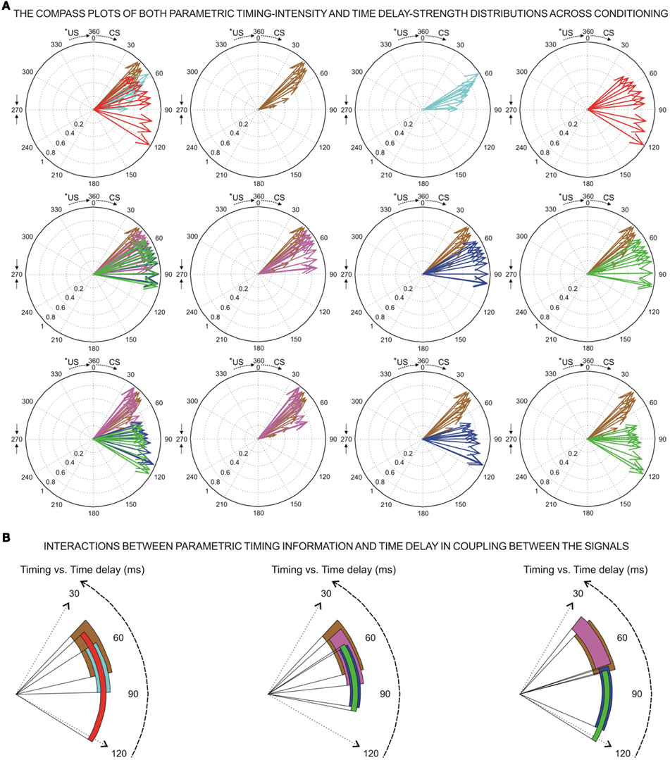
Figure 7. (A) The compass plots of both parametric timing–intensity and time delay–strength distributions across the 10 conditioning sessions, and for the simulated time condition ^*ISI = 360 ms. In this representation, the timing–intensity distributions (1) [time to CR onset, percentage of CR], see brown arrows, and (2) [time to peak firing rate of the IP neurons, IPn peak firing rate], see cyan arrows, and the time delay–strength distributions (3) [time delay in coupling τ0_{〈f|IP|θ〉}, maximum linear correlation coefficient r_{max〈f IP | θ〉}], see red arrows, (4) [τ1_{〈EMG | MN〉}, η1_{max 〈EMG | MN〉}] and (5) [τ2_{〈MN | EMG〉}, η2_{max 〈MN | EMG〉}], see magenta arrows, (6) [τ3_{〈EMG | IP〉}, η3_{max 〈EMG | IP〉}] and (7) [τ4_{〈IP | EMG〉}, η4_{max 〈IP | EMG〉}], see blue arrows, and (8) [τ5_{〈MN | IP〉}, η5_{max 〈MN | IP〉}] and (9) [τ6_{〈IP | MN〉}, η6_{max 〈IP | MN〉}], see green arrows, were plotted using the circular statistics. The 10 colored arrows (10 conditioning sessions, C01–C10) in each circle illustrate the circular dispersion of the angular datasets represented. The first row of circles shows the parametric timing–intensity dispersion patterns, and the second and third rows of circles show the time delay–strength circular distributions across conditioning sessions (see the dispersion parameters in Table 3). (B) Interactions between parametric timing information and time delays in coupling between the physiological signals. The colored circular sectors illustrate the time-dispersion range of the data distributions represented in (A) (see the dispersion parameters in Table 2).

TABLE 3

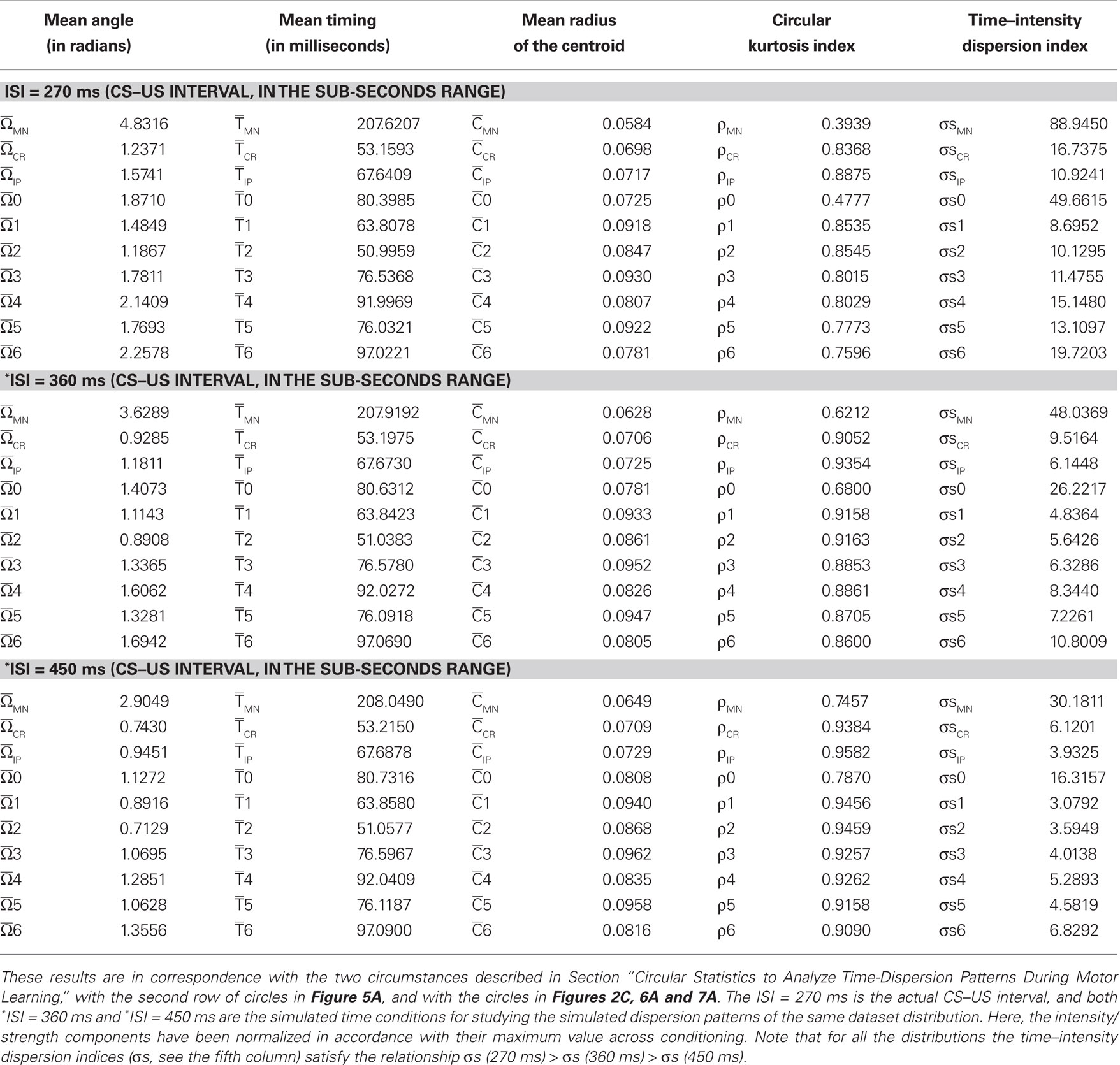
Table 3. The parametric timing–intensity and time delay–strength dispersion indices (σs) corresponding to the circular distributions of the datasets across conditioning sessions, and for three different durations of the inter-stimulus interval (ISI).

TABLE 4

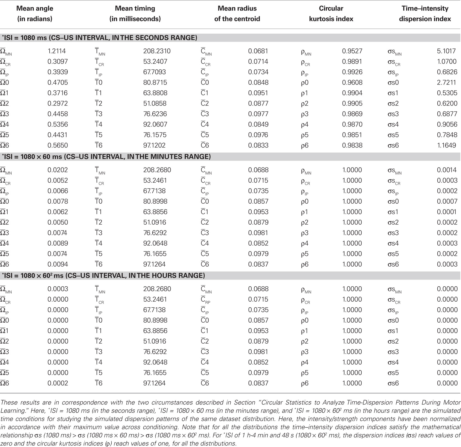
Table 4. The parametric timing–intensity and time delay–strength dispersion indices (σs) corresponding to the circular distributions of the datasets across conditioning sessions, and for three different durations of the inter-stimulus interval (ISI).

These intra- and inter-trial timing strategies extending from sub-second range (millisecond timing, for the intra-trial domain) to seconds-to-minutes-to-hours range (interval timing, for the inter-trial and inter-block domains) expanded the functional domain of cerebellar timing beyond motor control. In fact, we calculated the different dispersion indices (σs) to reveal the true parametric timing–intensity (and time delay–strength) dispersion patterns between the IPn activity and either Mn or OO EMG recordings in the different temporal domains (inter-trials dispersion of the same block, inter-blocks dispersion of the same session, and inter-sessions dispersion along the process) – i.e., the time–intensity contributions (at least in the circular statistical sense) of the different neuronal centers (cerebellar interpositus and facial nuclei) participating in this associative learning process. It could thus be concluded that the firing activities of IPns and their temporal dynamics may be related more with the proper performance of ongoing CRs (including the proper parametric timing–intensity and time delay–strength dispersion patterns) than with their generation and/or initiation.

Relationships between Phase Synchronization and Both Timing and Causality in the Cerebellar–Motoneuron Network

A question of great interest is whether there is a “causal” relationship between two simultaneous recordings collected during associative motor learning without any specific information on the direction of the coupling or on the time-dispersion pattern of the physiological data. The linear cross-correlation function, the non-linear association method, and the circular dispersion approach are, in principle, able to indicate the time delays in coupling and their circular distributions, but inferring causality from the mere directionality or the time-dispersion pattern is not always straightforward (Granger, 1980; Lopes da Silva et al., 1989; Pereda et al., 2005). Therefore, we decided to investigate the putative functional interdependencies between neuronal activity [firing rates of OO Mns, f_MN(t), or IPns, f_IP(t)] and learned motor responses [i.e., conditioned eyelid responses, θ(t)], using time-dependent causality analysis (see Time-Dependent Causality Analysis Between Neuronal Firing Command and Learned Motor Response, and Sánchez-Campusano et al., 2009 for details).

The physiological time series f_MN(t), f_IP(t), and θ(t) exhibit non-stationary behaviors. The stationary time series S1_t (MN), S2_t (IP), S3_t (SUM), and S0_t (θ) were determined here by successive regular differentiation of averaged relative variation functions and afterward by high-pass filtering of integrated neuronal firing activities [resulting from f_MN(t) for Mns, and from f_IP(t) for IPns] and of learned motor responses [resulting from eyelid position θ(t) during conditioned eyelid responses, CRs; see Sánchez-Campusano et al., 2007 for details]. From here on, the significant values of the transfer function (or sample impulse response) are those that are outside the confidence bounds (horizontal red dashed lines, approximately 95% confidence interval), indicating the number of SD of the sample impulse response estimation error to compute, assuming that the input and output physiological time series are uncorrelated. The causal inferences between the kinetic neuronal commands [S1_t (MN), for the activity of OO Mns; and S2_t (IP), for the activity of IPns] and the kinematics [S0_t (θ), for CRs] were determined using the normal and normalized Granger causality indices. Readers may refer to the above-mentioned reports for a detailed and practical description of this technique.

In Figures 7 and 8 are represented transfer function models (TFM) for the physiological time series corresponding to data collected from the 10th conditioning session, in particular, the activities of three representative IPns and a representative Mn were selected for each experimental subject (n = 8; Series S1: C10, 4 cats, 4 Mns; Series S2: C10, 4 cats, 12 IPns). For the curves shown in Figure 8A, the significant values of the transfer function presented a bimodal distribution for both positive (ν_k+ ≠ 0) and negative (ν_k− ≠ 0) lags, indicating that S0_t (θ) depends on its own past and on the past of S2_t (IP), whilst S2_t (IP) depends on its own past and on the past of S0_t (θ). That is, significant values of the causality indices in both senses (G_{2 → 0} > 0 and G_{0 → 2} > 0) indicate a bidirectional coupling or feedback relationship between these time series. At the same time, and as illustrated in Figure 8B, the functional coupling (or feedback relationship, the same as in Figure 6A) between S1_t (MN) and S2_t (IP), was bidirectional in the sense of Granger causality (G_{2 → 1} > 0, G_{1 → 2} > 0, ν_k+ ≠ 0 and ν_k− ≠ 0), and these causal inferences signify that the neuronal activity in the posterior IP nucleus causes both the activity present in the final common pathway (i.e., that of the Mns participating in the generation of the selected motor responses) and the CRs of the eyelid motor system, and vice versa [S1_t (MN) depends on its own past and on the past of S2_t (IP), and S2_t (IP) depends on its own past and on the past of S1_t (MN)].

FIGURE 8

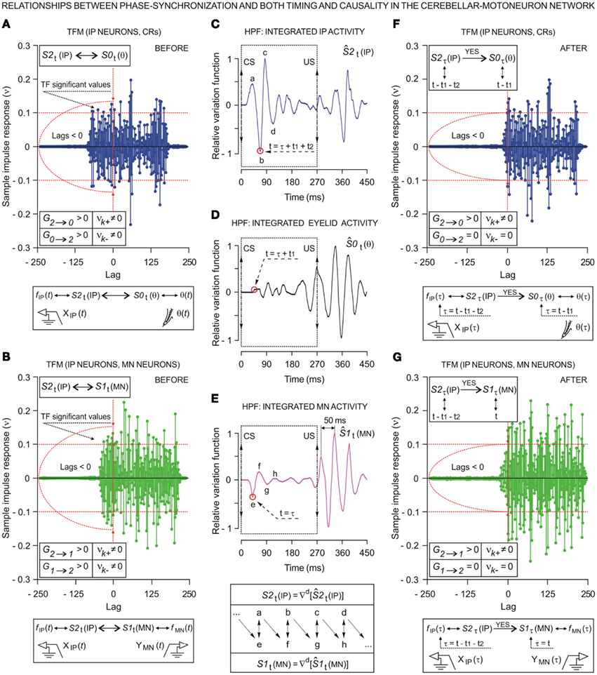
Figure 8. Relationships between phase synchronization and both timing and causality in the cerebellar–Mn network using transfer function models (TFM) between kinetic neuronal commands of the IP neurons (IPn) and motor activities [activity of OO Mns (Mn) and eyelid CRs], before [see (A,B)] and after [see (F,G)] the phase synchronization as a simulated causal condition [see (C–E)]. (A,B) Before the phase synchronization, the transfer function models assume that the stationary time series S1_t (MN), S2_t (IP) and S0_t (θ) have a functional and dynamic relationship. In (A), the causality indices are such that G_{2 → 0} > 0 and G_{0 → 2} > 0, ν_k+ ≠ 0 and ν_k− ≠ 0 – i.e., S0_t(θ) depends on its own past and on the past of S2_t(IP), and S2_t(IP) depends on its own past and on the past of S0_t(θ). In (B), S1_t(MN) depends on its own past and on the past of S2_t(IP), and S2_t(IP) depends on its own past and on the past of S1_t(MN) – i.e., significant values of the causality indices in both senses: G_{2 → 1} > 0, G_{1 → 2} > 0, ν_k+ ≠ 0 and ν_k− ≠ 0. The transfer function models in (A,B) indicate the feedback relationships between IPn time series S2_t (IP) and either S0_t (θ) or S1_t (MN), at least in the statistical sense of causality. (C–E) Oscillatory curves (relative variation functions) resulting from high-pass filtering (HPF, –3 dB cutoff at 5 Hz and zero gain at 15 Hz) of integrated neuronal firing activities (IPn and Mn) and of eyelid position corresponding to the same set of records. The operator £^d enabled the stationary time series S1_t (MN), S2_t (IP), and S0_t (θ) to be obtained after making n = d regular differentiations to the non-stationary time series [i.e., the relative variation curves, as shown in (C–E)]. Note that in the oscillating curves shown here, components a–d are totally out-of-phase with components e–h. The transfer function models (F,G) assume that the stationary time series possess a direct interdependence after phase synchronization as a simulated causal condition [i.e., the phases corresponding to τ = t − t1 − t2, for S2_τ (IP), τ = t − t1, for S0_τ (θ), and τ = t, for S1_τ (MN)], implying that S0_τ (θ) depends on its own past and on the past of S2_τ (IP) (i.e., the indices are such that G_{2 → 0} > 0 and G_{0 → 2} = 0, ν_k+ ≠ 0 and ν_k− = 0, see F for a unidirectional coupling); and that S1_τ (MN) depends on its own past and on the past of S2_τ (IP) (i.e., G_{2 → 1} > 0, G_{1 → 2} = 0, ν_k+ ≠ 0, and ν_k− = 0, see the panel G for another unidirectional coupling). Red horizontal dashed lines in (A,B) and (F,G) indicate the approximate upper and lower confidence bounds (approximately 95% confidence interval), assuming the input and output physiological time series are completely uncorrelated.

The transfer function models shown in Figures 8F,G assume that the stationary time series [S2_τ (IP) and S2_τ (θ), as shown in Figure 8F, or S2_τ (IP) and S1_τ (MN), as indicated in Figure 8G], possess a unidirectional interdependence after phase synchronization as a simulated causal condition. Thus, the relationships between phase synchronization and both timing and causality in the cerebellar–Mn network were explored at the millisecond scale – i.e., taking into account the Mn and IPn spike timing. The phase corresponding to S2_τ (IP) in the instant τ = t − t1 − t2 was equivalent to the phases corresponding to S0_τ (θ) and S1_τ (IP) in the instants τ = t − t1 and τ = t, respectively, as illustrated in Figures 8C,D. The actual values for t1 (time elapsed from activation of Mn firing to the zero reference point – i.e., the start of the CR, see Figure 2A) and t2 (time elapsed from the zero reference point to the activation of IPn firing) were 5.98 ± 0.26 (mean ± SEM, range, 3.41–8.56) ms and 23.5 ± 0.31 (mean ± SEM, range, 20.41–26.59) ms, respectively. With these simulated causal conditions of phase synchronization, the Granger causality indices are such that G_{2 → 0} > 0 and G_{0 → 2} = , ν_k+ ≠ 0 and ν_k− = 0 (see Figure 8F), implying that S0_τ (θ) depends on its own past and on the past of S2_τ (IP); and G_{2 → 1} > 0, G_{1 → 2} = 0, ν_k+ ≠ 0, and ν_k− = 0 (see Figure 8G), which signifies that S1_τ (MN) depends on its own past and on the past of S2_τ (IP). This phase analysis demonstrates that causal inferences are dependent on the phase information status, as indicated in Figures 8F,G.

As illustrated in Figure 9A, the functional interdependence between S0_t (θ) and S1_t (MN) was unidirectional (significant values of the transfer function alone for lags >0, ν_k+ ≠ 0 and ν_k− = 0) – i.e., the Granger causality indices are such that G_{2 → 0} > 0 and G_{0 → 1} = 0, which signifies that S0_τ (θ) depends on its own past and on the past of S1_t (MN) and, as a result, OO Mns consistently lead the OO muscle during conditioned eyelid responses. In contrast, the relationship between S0_τ (θ) and S3_τ (SUM) was unidirectional (G_{3 → 0} > 0, G_{0 → 3} = 0, ν_k+ ≠ 0 and ν_k− ≠ 0), which indicates that this causal inference is dependent on the phase information, as shown in Figure 9D.

FIGURE 9

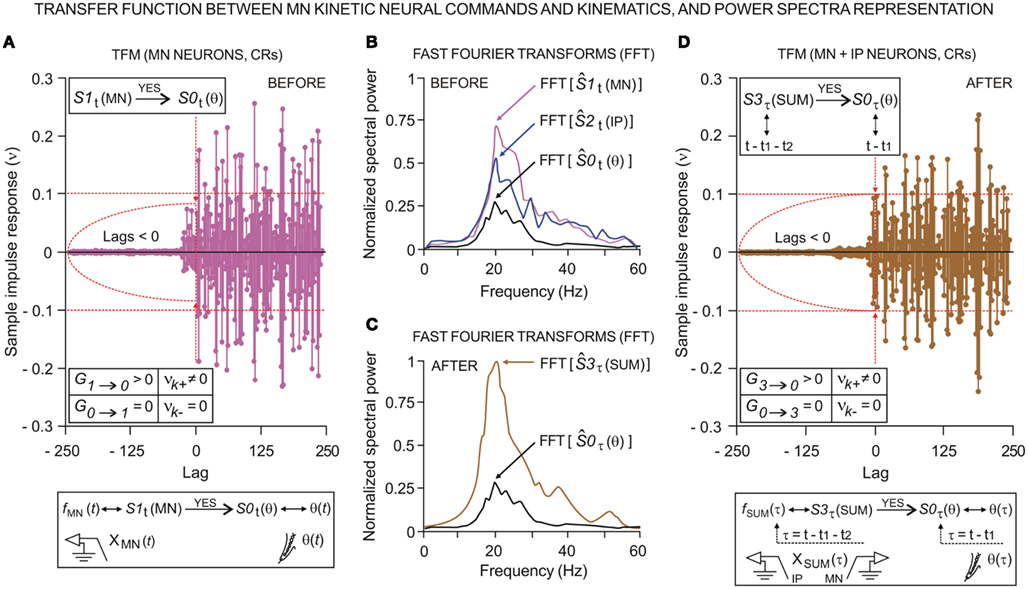
Figure 9. Transfer function models (TFM) between Mns kinetic neuronal commands and conditioned eyelid responses, before [see (A)] and after [see (D)] the phase synchronization as a simulated causal condition. In (A), the transfer function model establishes that the stationary time series S0_t (θ) depends on its own past and on the past of S1_t (MN) – i. e., the causality indices are such that G_{1 → 0} > 0 and G_{0 → 1} = 0, ν_k+ ≠ 0 and ν_k− = 0, indicating a unidirectional coupling in the final motor pathway of eyelid motor response. (B,C) Fast Fourier Transforms (FFT) for the oscillating curves shown in Figures 8C–E, before [see (B)] and after [see (C)] the phase synchronization (the sum of the contributions is possible only assuming both the frequency and phase synchronizations). Note that the illustrated spectra presented a significant predominance of spectral components at ≈ 20 Hz, and significant differences between their power spectra [F_{(3, 9, 236)} = 25.81, P < 0.01]. In (D), the causality indices are such that G_{3 → 0} > 0, G_{0 → 3} = 0, ν_k+ ≠ 0 and ν_k− = 0, also indicating a unidirectional coupling. Note that S3_τ (SUM) depends only on its own past (i.e., G_{0 → 3} = 0), and that the unidirectional relationship in the opposite direction [as shown in (D)] was possible because S1_t (MN) and S2_τ (IP) were induced toward a phase synchronization as a simulated causal condition (i.e., the relative phase difference will be close to zero for the S1_τ (MN) and S2_τ (IP) signals). Red horizontal dashed lines in A and D indicate the approximate upper and lower confidence bounds (approximately 95% confidence interval), assuming the input and output physiological time series are completely uncorrelated.

Finally, the maximum amplitude of the Mn relative variation function was significant [F_{(9, 27, 98)} = 170.26, P < 0.01] both in the CS–US interval and after the US presentation. Furthermore, the oscillation amplitude of the IPn relative variation function increased progressively across the learning process, reaching significant values [F_{(9, 27, 98)} = 59.51, P < 0.01] during the 10th conditioning session (Figures 8C–E). Furthermore, the illustrated spectra (Figures 9B,C) presented a significant predominance of spectral components at ≈ 20 Hz, and significant differences between their spectral power [F_{(3, 9, 236)} = 25.81, P < 0.01] at the asymptotic level of acquisition of this associative learning test (session C10). In addition, we found significant differences in the power spectra for both Mns S1_t (MN) [F_{(9, 27, 98)} = 225.48, P < 0.01] and IPns S2_τ (IP) [F_{(9, 27, 98)} = 216.28, P < 0.01] physiological time series across conditioning sessions.

Discussion

Design of Optimized Experimental and Analytical Tools to Analyze Timing, Time Delays, and Causality during Motor Learning

The multivariate analyses of physiological signals (non-linear dynamic associations and time-dependent Granger causality), the circular statistics of the dataset distributions, and the hierarchical cluster technique are optimal analytical tools for studying the interactions among timing parameters (i.e., the latencies and relative refractory periods, Figure 3A), kinetic neural commands (i.e., motor and pre-motor neuronal activities, Figure 3B), kinematic variables (i.e., motor activities computed from actual eyelid movement and their quantitative evolution, Figures 3B,C), correlation codes (i.e., the type and strength in coupling, Figures 4A,B), time delay information (i.e., the temporal order, Figures 6B and 7B), dispersion patterns (i.e., time–intensity circular distributions, Figures 5A–7A), and finally, the directionality/causality indices (Figures 8 and 9) conforming the 40-dimension vectors of learning states (Figure 10A) during motor learning. The results used here enable us to determine the intrinsic coherence (Figure 10B) of collected data and the relationship between timing and causality in the cerebellar–Mns network in different temporal domains (in the range of milliseconds for intra-trials interactions; in the range of seconds, minutes, and hours for both inter-trials and inter-blocks interactions; and in the range of days for the inter-sessions interactions along the process). For this, we have developed the necessary computer programs and algorithmic procedures to deal with such a huge amount of data (40 parameters quantified across 180 averaged blocks and 15 experimental sessions collected from 8 experimental animals). The computer program arranged the data in a total of 180 blocks (15 conditioning sessions × 12 blocks) according to their significant homogeneity: namely, blocks within clusters were displayed close together when plotted geometrically according to linkage distances, whereas different clusters were displayed far apart.

FIGURE 10

Figure 10. (A) Schematic representation of a parametric vector corresponding to the learning state for a given training block. The diagram illustrates the qualitative definition of a 40-dimension state vector formed by 5 timing parameters (from 1 to 5, see Figure 3A), 4 kinetic neural commands (from 6 to 9, see Figure 3B), 2 kinematic variables (10 and 11, Figure 3B), 7 correlation code parameters (from 12 to 18, see Figure 4A), 7 time delays (from 19 to 25, Figure 6B), 9 dispersion patterns (from 26 to 34, Figures 5A and 6A, and Table 3), and finally 6 directional and causality indices (from 35 to 40, Figures 8 and 9). A color map representation of the parametric vector (the horizontal blue arrow) is also illustrated. Note the alternation of ranges of colors describing in qualitative and quantitative terms a functional state of the cerebellar–Mn pathway during motor learning. (B) Hierarchical cluster trees of averaged blocks using the 40-dimension vectors of learning states collected across habituation (H01–H02), conditioning (C01–C10), and extinction (E01–E03) sessions. The dendrograms illustrate the hierarchical distributions of the averaged blocks of trials across the classical conditioning and in accordance with both actual (the left-hand dendrogram, D1) and simulated (the right-hand dendrogram, D2) causality inferences. Each bar at the bottom of the dendrograms represents an averaged conditioning block. The linkage-weighted distances between the vectors are represented on the x-axes in arbitrary units. The comparison depth was of 16 levels to both sides of the objective level, and the clusters were formed without specifying the maximum number of clusters. The y-axes represent, as colored (not black) lines, the statistically significant clusters [D1, 15 significant clusters, 147 averaged blocks, F_{(14, 70, 132)} = 36.1213, P < 0.01, Wilk’s lambda = 0.09, with Nr = 5; D2, 10 significant clusters, 166 averaged blocks, F_{(9, 45, 156)} = 2.4290, P < 0.05, Wilk’s lambda = 0.26, with Nr = 5]. The black lines represent the averaged blocks (33, in D1; 14 in D2) that fall into the remaining statistically non-significant clusters (16 in D1; 4 in D2). According to the left-hand dendrogram D1 (for the actual causality inferences), the 15 significant clusters corresponded to 147 averaged blocks distributed in the 15 experimental sessions during the delay conditioning paradigm (H01–H02 = 19, C01–C10 = 108, and E01–E03 = 20 blocks). Here, notice a coherent nodal distribution (see the vertical colored bars in the left-hand panel) in correspondence with a proper trend in the evolution of the conditioning process. However, for the right-hand dendrogram D2 (simulated causality inferences), the total number of significant clusters was of 10 groups – i.e., an insufficient number of groups to match with the 15 conditioning sessions. Note that in D2 the clusters were obtained with evident linkage alterations that affect the typical and sequential temporal distribution of training blocks (see the yellow and pink horizontal bars) and sessions (see the vertical colored bars in the right nodal distribution) along the conditioning process. The green and red vertical dashed lines indicate the threshold linkage distances (46.57 and 117.94 units for D1 and D2, respectively) for these hierarchical cluster distributions.

The main result according to the actual causality inferences (see the left-hand hierarchical cluster trees in Figure 10B) indicated that up to 147 blocks could be correctly assigned to the corresponding experimental (habituation, conditioning, or extinction) session, and only data collected from 33 blocks were discarded because of their low homogeneity with the corresponding session. Here, the threshold linkage distance was of only 46.57 units (see the vertical green dashed line) and the hierarchical cluster trees were significantly consistent (high cophenetic correlation coefficient, 0.9802; the closer this value is to 1, the better the clustering) with the actual conditioning sessions. For example, and given the similarity of the data collected in the corresponding trials and blocks, the two habituation sessions (H01, H02) were clustered close to the 1st conditioning session (C01). In addition, the 1st extinction session (E01) was clustered close to the 10th conditioning session (C10), while the following extinction sessions (E02, E03) were clustered close to the C07–C09 conditioning sessions. Finally, the middle experimental sessions (C02–C06) formed a distinct set of clusters. Importantly, these positive results indicated that neural firing properties recorded from different animals during the same conditioning paradigm can be correctly assigned to the corresponding experimental session (i.e., in agreement with the actual CR evoked during the CS–US interval).

However, for the simulated causality conditions (see the right-hand hierarchical cluster trees in Figure 10B), where only the directionality and causality indices that involved the IPn interdependencies were modified randomly (sequence of 0 or 1 for the parameters 36, 37, 39 and 40 of each averaged block, in Figure 10A) prior to application of the clustering algorithm, the clusters were obtained with evident linkage alterations and inconsistency (moderate cophenetic correlation coefficient, 0.6836) affecting the typical and sequential temporal distribution of training blocks (see the yellow and pink horizontal bars) and experimental sessions (see the vertical colored bars in the right nodal distribution) along the conditioning process. For example, (1) the formation of two independent groups (see the first pink and yellow arrows and the indicated bars) for the same conditioning session C01; (2) the high similarity between two different experimental sessions (C02 and C03, see the second pink arrow and the indicated bar), and the significant similarity of them with the session C05; (3) the high similarity between the conditioning session C06 and the extinction sessions E01–E03 (see the second yellow arrow and the indicated bar); and finally, the high homogeneity of linkage for three experimental conditioning sessions (C07, C09, and C10, see the third pink arrow and the indicated bar) which showed significant differences for the actual causality inferences. Furthermore, note that in the right-hand dendrogram D2 for averaged blocks and in the right nodal distribution for sessions, the total number of significant clusters was of 10 groups – i.e., an insufficient number of clusters to match with 15 experimental conditioning sessions. Moreover, the threshold linkage distance was 117.94 units (see the vertical red dashed line) – i.e., a linkage distance that does not allow a valid rejection of the non-significant data corresponding to averaged blocks.

This strategy of the simulated causality conditions by a controlled random modification of the directionality and causality inferences (the parameters 36, 37, 39, and 40, which involved IPn interdependencies, Figure 10A) in the temporal domains of the inter-trials and inter-sessions interactions strongly suggests that the proper timing of CRs is plausibly a consequence of the pertinent cerebellar–Mn network causality (Figures 8–10) – i.e., the simulated causal conditions affect the typical temporal distribution of training blocks and experimental sessions along the conditioning process, and therefore the temporal evolution of the level of expression of eyelid CRs. In the temporal range of interval timing (seconds-to-minutes-to-hours) these dynamic changes were determined by the emergence of spurious causality interdependencies from inter-blocks data interactions to inter-sessions data interactions. At the milliseconds scale the spikes timing (the dynamic firing properties of the Mns and IPns) was also modified by an induced sequence of phase synchronization (i.e., the relative phase difference will be close to zero). Indeed, as shown in a previous study from our group (Sánchez-Campusano et al., 2007, 2009), the reinforcing-modulating role of cerebellar circuits of ongoing conditioned eyelid responses is highly dependent on its adequate phase-modulation with respect to intrinsic facial Mn oscillatory properties. To be efficient, IPn activities need to go through a learning process to become 180° out-of-phase OO Mns firing (Sánchez-Campusano et al., 2007). Thus, IPn activities (following a relay in the red nucleus) reach OO Mns right at the moment of maximum motoneuronal hyperpolarization (Trigo et al., 1999), and IPns facilitate a quick repolarization of OO Mns, reinforcing their tonic firing during the performance of eyelid CRs (Sánchez-Campusano et al., 2009).

An additional advantage of this approach is that for the actual causality conditions, once collected data were properly arranged according to the hierarchical cluster tree (and that non-significant data were rejected), it was possible to determine analytically the multiple and coherent evolution of timing parameters (Figure 3A), kinetic and kinematic variables (Figures 3B,C), the dynamic non-linear association functions relating Mn and IPn activities to EMG responses (Figure 4), the time–intensity dispersion patterns (Figures 5–7) of the dataset distributions in the CS–US interval using circular statistics, and – finally – the relationship between the causal inferences and phase-inversion properties (Figures 8 and 9) of OO Mns and IPns with regard to acquired CRs. This phase-synchronization analysis demonstrates that causal inferences are dependent on the phase information status and that the timing of learned eyelid responses depends on the causal relationships present in the cerebellar–Mn network. Finally, these novel (experimental and analytical) approaches to the study of actual neuronal mechanisms underlying the acquisition of new motor abilities will certainly contribute to the better understanding of brain functioning in alert behaving animals.

A More Precise Picture of the Functional States Involved in the Actual Acquisition of New Motor and Cognitive Abilities

Our intention here was to deal with the putative cerebellar nuclear mechanisms involved in the acquisition and performance of conditioned eyeblinks, compared with the role play by facial motoneurons. In this regard, and according to a long series of studies carried out by some of us in alert behaving cats, posterior interpositus neurons fire in response to every type of eyelid displacement: spontaneous, reflex, or classically conditioned with either delay or trace paradigms. In contrast such an activity was not detected in other interpositus areas (Gruart and Delgado-García, 1994; Gruart et al., 2000a; Delgado-García and Gruart, 2002). Previous electrophysiological recordings of putative cerebellar nuclei units carried out in rabbits reported that eyeblink-related neurons are located in the rostral part of the interpositus nucleus (McCormick and Thompson, 1984; Berthier and Moore, 1990). However, and in agreement with recordings carried out in behaving monkeys (Van Kan, et al., 1993), a detailed mapping of the three cerebellar nuclei in alert behaving cats indicates that neurons related to eyelid movements are mostly located in the rostro-dorso-lateral aspect of the posterior interpositus nucleus (Gruart and Delgado-García, 1994; Gruart et al., 2000). Moreover, data collected from mice (Porras-García et al., 2010) and rats (Morcuende et al., 2002; Chen and Evinger, 2006) also located eyeblink-related neurons in the dorsolateral hump and in the posterior interpositus nucleus, but not in the anterior subdivision of the nucleus. Until now, there is no better explanation for these disparities in the location of eyeblink-related neurons that the possible neural differences within different species. On the other hand, we have analyzed here just the firing activities of interpositus type A neurons (Gruart et al., 2000). In a forthcoming study, we will analyze in detail the firing properties of interpositus type B neurons (i.e., neurons that pause during the CS–US interval; Gruart et al., 2000), as well as the discharge rates of overlying type A and B Purkinje cells (in preparation).

In a recent work from our group (Sánchez-Campusano et al., 2010) we presented a quantitative statistical analysis of several separate but similar experiments in order to test the pooled data for statistical significance revealing how IPns can change their activity during delayed eyeblink conditioning. That previous meta-analysis enabled a comparison for learning and performance in different species. The present experimental design in alert behaving cats (for a single animal species) enables the incorporation of further parameters (timing information, time delays, time–intensity dispersion patterns, directionality in coupling, and causality indices) with the sole condition that the same experimental conditioning situation is reproduced (i.e., the same delay conditioning paradigm). Although we have checked here the firing characteristics of only OO Mns and IPns, the intrinsic coherence demonstrated among timing information, kinetic and kinematic parameters, time delays and correlation code properties, time–intensity dispersion patterns, directional outcomes, and causality inferences conforming the 40-dimension vectors of learning states (Figure 10A) strongly suggests the presence of a functional neuronal state involving many different cerebral centers evoked by the learning process (Delgado-García and Gruart, 2002; Sánchez-Campusano et al., 2007, 2009, 2010).

The recent demonstration of the existence of the “brain states” (Petersen, 2007; Poulet and Petersen, 2008; Crochet et al., 2011) determined by oscillation of the membrane potential in synchronized pyramidal cells may be compared with our experimental data showing similar oscillations in the OO Mns (Trigo et al., 1999). Thus, in the cerebellar–Mns network the oscillations of IPns (modulating signal) modulates and/or reinforces eyelid motor responses inversely (by progressively inverting phase information) to the initial contribution of OO Mns (modulated signals). In previous reports (Gruart and Delgado-García, 1994; Gruart et al., 2000a; Sánchez-Campusano et al., 2007, 2009), we demonstrated by different means that neuronal activity in the IP nucleus does not lead the performance of learned motor responses, but follows neural motor commands originated in different neuronal sources. Although it is highly speculative at the moment, we can suggest that a driving common source in motor cortex and/or in related cortical areas could act as both a trigger and a distributor of significant functional information in relation with the timing and performance of conditioned eyelid responses. As a whole, IPns could be considered to behave as a neuronal phase-modulating device supporting OO Mns firing during learned eyelid movements.

Furthermore, according to the recently reviewed general principles of the brain network (De Zeeuw et al., 2011), the spatiotemporal coding, in addition to firing rate coding, might support cerebellar processing. These spatiotemporal patterns (firing rate, and spike timing) may be compared with our results showing parametric timing–intensity and time delay–strength dispersion patterns of the neurons at different timescales – i.e., the spike-rate code, the spike-timing code, and correlation code (the strength and type of interdependence between signals, including the asymmetry information) – all together as a central spatiotemporal pattern. In the milliseconds range (intra-trial interaction), the firing properties of the IPns (i.e., the peak firing rate and the total number of spikes in the CS–US interval), the parametric timing (i.e., the time to peak firing and relative refractory periods), the time delay in coupling (i.e., the time to maximum correlation code between the neuronal recordings), the time–intensity dispersion patterns, and – finally – the causality inferences (correlation code and temporal order) were conforming a more exhaustive spatiotemporal pattern or a more precise picture of the functional states involved in the actual acquisition of new motor and cognitive abilities. In this paper, the results of the causal analyses for the time-dependent relative variation functions of the IPns and OO Mns firing rates (Figures 8 and 9) enabled investigation of the relationship between the relevance of spike timing and the novel spatiotemporal pattering (as a neuronal state vector at the milliseconds timescale) characterizing the firing properties and their dynamic patterns (time-dispersion and temporal evolution), as well as the strength of the interdependencies between neuronal activities and the performance (kinematics) of eyelid conditioned responses. This idea was extended to inter-trials, inter-blocks (Figure 10A), and inter-sessions (Figure 10B) interactions of the datasets using the corresponding averaged firing rates of IPns and OO Mns and their causality interdependencies (all as a more exhaustive averaged spatiotemporal pattern) to study the timing of averaged eyelid CRs, the sequential temporal distribution of averaged datasets corresponding to averaged blocks and experimental sessions along the conditioning process.

Finally, the same experimental protocols and analytical procedures (including as an essential method the circular distribution of the experimental data) could also be applied to different durations of CS–US interval as an alternative approach to provide interval-based representations in order to understand better the interval timing mechanisms. In the first instance, the simulated time conditions where the data distribution is fitted to the circle may be extended to the standard interval timing strategy with the aim of exploring the quantifiable changes in the time–intensity dispersion patterns of data distributions depending on the duration of the CS–US interval. In the second instance, these experimental and analytical approaches could also be applied to many pharmacological manipulations that modify the spatiotemporal firing pattern (spike rate, spike timing, and correlation codes) within the cerebellar-IP nucleus-red-nucleus-Mns network. These modifications in the spatiotemporal patterns lead to a dynamic change in the functional neuronal state (timing and their corresponding kinetic neural commands and dispersion patterns) evoked by the learning process, and consequently to some change in the timing and performance of the learned motor responses – i.e., in the motor behavior.

Conflict of Interest Statement

The authors declare that the research was conducted in the absence of any commercial or financial relationships that could be construed as a potential conflict of interest.

Acknowledgments

Work supported by grants MICINN-BFU2008-0899, P07-CVI-2487 and JA-BIO-122 to José M. Delgado-García, and MICINN-BFU2008-03390 and P07-CVI-02686 to Agnès Gruart. We thank Roger Churchill for his editorial help.

References

Aksenova, T. I., Chibirova, O. K., Dryga, O. A., Tetko, I. V., Benabid, A. L., and Villa, A. E. P. (2003). An unsupervised automatic method for sorting neuronal spike waveforms in awake and freely moving animals. Methods 30, 178–187.

Pubmed Abstract | Pubmed Full Text | CrossRef Full Text

Almeida, R., and Ledberg, A. (2010). A biologically plausible model of time-scale invariant interval timing. J. Comput. Neurosci. 28, 155–175.

Pubmed Abstract | Pubmed Full Text | CrossRef Full Text

Batschelet, E. (1981). Circular Statistics in Biology New York: Academic Press.

Berens, P. (2009). CircStat: a MATLAB toolbox for circular statistics. J. Stat. Softw. 31, 1–21.

Berman, A. L. (1968). The Brain Stem of the Cat: A Cytoarchitectonic Atlas with Stereotaxic Coordinates Madison, WI: University of Wisconsin Press.

Berthier, N. E., and Moore, J. W. (1990). Activity of deep cerebellar nuclear cells during classical conditioning of nictitating membrane extension in rabbits. Exp. Brain Res. 83, 44–54.

Pubmed Abstract | Pubmed Full Text | CrossRef Full Text

Box, G. E. P., and Jenkins, G. M. (1976). Time Series Analysis: Forecasting and Control San Francisco: Holden-Day.

Brown, E. N., Kass, R. E., and Mitra, P. P. (2004). Multiple neural spike train data analysis: state-of-the-art and future challenges. Nat. Neurosci. 7, 456–461.

Pubmed Abstract | Pubmed Full Text | CrossRef Full Text

Buhusi, C. V., and Meck, W. H. (2005). What makes us tick? Functional and neural mechanisms of interval timing. Nat. Rev. Neurosci. 6, 755–765.

Pubmed Abstract | Pubmed Full Text | CrossRef Full Text

Buonomano, D. V., and Karmarkar, U. R. (2002). How do we tell time? Neuroscientist 8, 42–51.

Pubmed Abstract | Pubmed Full Text | CrossRef Full Text

Buonomano, D. V., and Laje, R. (2010). Population clocks: motor timing with neural dynamics. Trends Cogn. Sci. (Regul. Ed.) 14, 520–527.

Pubmed Abstract | Pubmed Full Text | CrossRef Full Text

Chan, H. L., Wu, T., Lee, S. T., Fang, S. C., Chao, P. K., and Lin, M. A. (2008). Classification of neuronal spikes over the reconstructed phase space. J. Neurosci. Methods 168, 203–211.

Pubmed Abstract | Pubmed Full Text | CrossRef Full Text

Chen, F. P., and Evinger, C. (2006). Cerebellar modulation of trigeminal reflex blinks: interpositus neurons. J. Neurosci. 26, 10569–10576.

Pubmed Abstract | Pubmed Full Text | CrossRef Full Text

Clarke, S., Ivry, R., Grinband, J., Roberts, S., and Shimizu, N. (1996). “Exploring the domain of the cerebellar timing system,” in Time, Internal Clocks, and Movement, eds M. A. Pastor, and J. Artieda (New York: Elsevier), 257–280.

Crochet, S., Poulet, J. F., Kremer, Y., and Petersen, C. C. (2011). Synaptic mechanisms underlying sparse coding of active touch. Neuron 69, 1160–1175.

Pubmed Abstract | Pubmed Full Text | CrossRef Full Text

De Zeeuw, C. I., Hoebeek, F. E., Bosman, L. W., Schonewille, M., Witter, L., and Koekkoek, S. K. (2011). Spatiotemporal firing patterns in the cerebellum. Nat. Rev. Neurosci. 12, 327–344.

Pubmed Abstract | Pubmed Full Text | CrossRef Full Text

Delgado-García, J. M., and Gruart, A. (2002). The role of interpositus nucleus in eyelid conditioned responses. Cerebellum 1, 289–308.

CrossRef Full Text

Domingo, J. A., Gruart, A., and Delgado-García, J. M. (1997). Quantal organization of reflex and conditioned eyelid responses. J. Neurophysiol. 78, 2518–2530.

Pubmed Abstract | Pubmed Full Text

Domínguez-del-Toro, E., Rodríguez-Moreno, A., Porras-García, E., Sánchez-Campusano, R., Blanchard, V., Lavilla, M., Böhme, G. A., Benavides, J., and Delgado-García, J. M. (2004). An in vitro and in vivo study of early deficits in associative learning in transgenic mice that over-express a mutant form of human APP associated with Alzheimer’s disease. Eur. J. Neurosci. 20, 1945–1952.

CrossRef Full Text

Fiala, J. C., Grossberg, S., and Bullock, D. (1996). Metabotropic glutamate receptor activation in cerebellar Purkinje cells as substrate for adaptive timing of the classically conditioned eye-blink response. J. Neurosci. 16, 3760–3774.

Pubmed Abstract | Pubmed Full Text

Fisher, N. I. (1993). Statistical Analysis of Circular Data New York: Cambridge University Press.

Gallistel, C. R., and Gibbon, J. (2000). Time, rate, and conditioning. Psychol. Rev. 107, 289–344.

Pubmed Abstract | Pubmed Full Text | CrossRef Full Text

Geweke, J. (1982). Measurement of linear dependence and feedback between multiple time series. J. Am. Stat. Assoc. 77, 304–313.

CrossRef Full Text

Gibbon, J. (1977). Scalar expectancy-theory and Weber’s law in animal timing. Psychol. Rev. 84, 279–325.

CrossRef Full Text

Gibbon, J., and Church, R. M: (1990). Representation of time. Cognition 37, 23–54.

Pubmed Abstract | Pubmed Full Text | CrossRef Full Text

Gibbon, J., Malapani, C., Dale, C. L., and Gallistel, C. R. (1997). Toward a neurobiology of temporal cognition: advances and challenges. Curr. Opin. Neurobiol. 7, 170–184.

Pubmed Abstract | Pubmed Full Text | CrossRef Full Text

Grafen, A., and Hails, R. (2002). Modern Statistics for the Life Sciences New York: Oxford University Press Inc.

Granger, C. W. J. (1980). Testing for causality: a personal viewpoint. J. Econ. Dyn. Control 2, 329–352.

CrossRef Full Text

Grossberg, S., and Schmajuk, N. A. (1989). Neural dynamics of adaptive timing and temporal discrimination during associative learning. Neural Netw. 2, 79–102.

CrossRef Full Text

Gruart, A., Blázquez, P., and Delgado-García, J. M. (1995). Kinematics of unconditioned and conditioned eyelid movements in the alert cat. J. Neurophysiol. 74, 226–248.

Pubmed Abstract | Pubmed Full Text

Gruart, A., and Delgado-García, J. M. (1994). Discharge of identified deep cerebellar nuclei neurons related to eye blinks in the alert cat. Neuroscience 61, 665–681.

Pubmed Abstract | Pubmed Full Text | CrossRef Full Text

Gruart, A., Guillazo-Blanch, G., Fernández-Mas, R., Jiménez-Díaz, L., and Delgado-García, J. M. (2000a). Cerebellar posterior interpositus nucleus as an enhancer of classically conditioned eyelid responses in alert cats. J. Neurophysiol. 84, 2680–2690.

Gruart, A., Schreurs, B. G., Domínguez-del-Toro, E., and Delgado-García, J. M. (2000b). Kinetic and frequency-domain properties of reflex and conditioned eyelid responses in the rabbit. J. Neurophysiol. 83, 836–852.

Gruart, A., Muñoz, M. D., and Delgado-García, J. M. (2006). Involvement of the CA3-CA1 synapse in the acquisition of associative learning in behaving mice. J. Neurosci. 26, 1077–1087.

Pubmed Abstract | Pubmed Full Text | CrossRef Full Text

Hair, J. F., Anderson, R. E., Tatham, R. L., and Black, W. C. (1998). Multivariate Data Analysis New Jersey: Prince–Hall, Inc.

Harvey, A. (1994). Time Series I–II Cambridge: Cambridge University Press.

Ivry, R. B. (1996). The representation of temporal information in perception and motor control. Curr. Opin. Neurobiol. 6, 851–857.

Pubmed Abstract | Pubmed Full Text | CrossRef Full Text

Ivry, R. B., and Spencer, R. M. C. (2004). The neural representation of time. Curr. Opin. Neurobiol. 14, 225–223.

Pubmed Abstract | Pubmed Full Text | CrossRef Full Text

Jammalamadaka, S. R., and SenGupta, A. (2001). Topics in Circular Statistics Singapore: World Scientific Press.

Jarvis, M. R., and Mitra, P. P. (2001). Sampling properties of the spectrum and coherency in sequences of action potentials. Neural. Comput. 13, 717–749.

Pubmed Abstract | Pubmed Full Text | CrossRef Full Text

Jiménez-Díaz, L., Navarro-López, J. de D., Gruart, A., and Delgado-García, J. M. (2004). Role of cerebellar interpositus nucleus in the genesis and control of reflex and conditioned eyelid responses. J. Neurosci. 24, 9138–9145.

CrossRef Full Text

Kaminski, M., and Liang, H. (2005). Causal influence: advances in neurosignal analysis. Crit. Rev. Biomed. Eng. 33, 347–430.

CrossRef Full Text

Lejeune, H., and Wearden, J. H. (2006). Scalar properties in animal timing: conformity and violations. Q. J. Exp. Psychol. 59, 1875–1908.

CrossRef Full Text

Lewis, P. A., and Miall, R. C. (2003). “Overview: an image of human neural timing,” in Functional and Neural Mechanisms of Interval Timing, ed. W. H. Meck (Boca Raton, FL: CRC), 515–532.

Lewis, P. A., Miall, R. C., Daan, S., and Kacelnik, A. (2003). Interval timing in mice does not rely upon the circadian pacemaker. Neurosci. Lett. 348, 131–134.

Pubmed Abstract | Pubmed Full Text | CrossRef Full Text

Lopes da Silva, F. H., Pijn, J. P., and Boeijinga, P. (1989). Interdependence of EEG signals: linear vs. nonlinear associations and the significance of time delays and phase shifts. Brain Topogr. 2, 9–18.

Pubmed Abstract | Pubmed Full Text | CrossRef Full Text

Mardia, K. V. (1975). Statistics of directional data (with discussion). J. R. Stat. Soc. Series B Stat. Methodol. 37, 349–393.

Mardia, K. V., and Jupp, P. E. (1999). Directional Statistics Chichester: Wiley.

Matell, M. S., and Meck, W. H. (2004). Cortico-striatal circuits and interval timing: coincidence detection of oscillatory processes. Brain Res. Cogn. Brain Res. 21, 139–170.

Pubmed Abstract | Pubmed Full Text | CrossRef Full Text

Mauk, M. D., and Buonomano, D. V. (2004). The neural basis of temporal processing. Annu. Rev. Neurosci. 27, 307–340.

Pubmed Abstract | Pubmed Full Text | CrossRef Full Text

McCormick, D. A., and Thompson, R. F. (1984). Neuronal responses of the rabbit cerebellum during acquisition and performance of a classically conditioned nictitating membrane-eyelid response. J. Neurosci. 4, 2811–2822.

Pubmed Abstract | Pubmed Full Text

Meck, W. H. (1996). Neuropharmacology of timing and time perception. Brain Res. Cogn. Brain Res. 3, 227–242.

Pubmed Abstract | Pubmed Full Text | CrossRef Full Text

Meck, W. H., Penney, T. B., and Pouthas, V. (2008). Corticostriatal representation of time in animals and humans. Curr. Opin. Neurobiol. 18, 145–152.

Pubmed Abstract | Pubmed Full Text | CrossRef Full Text

Medina, J. F., Carey, M. R., and Lisberger, S. G. (2005). The representation of time for motor learning. Neuron 45, 157–167.

CrossRef Full Text

Miall, R. C. (1992). “Oscillators, predictions and time,” in Time, Action and Cognition: Bridging the Gap, NATO ASI Series D, Vol. 66, eds F. Macar, V. Pouthas, and W. Friedman (Dordrecht: Kluwer Academic Publishers), 215–227.

Miall, R. C. (1993). Neural networks and the representation of time. Psychol. Belg. 33, 255–269.

Morcuende, S., Delgado-García, J. M., and Ugolini, G. (2002). Neuronal premotor networks involved in eyelid responses: retrograde transneuronal tracing with rabies virus from the orbicularis oculi muscle in the rat. J. Neurosci. 22, 8808–8818.

Pubmed Abstract | Pubmed Full Text

Nolte, G., Ziehe, A., Nikulin, V. V., Schlögl, A., Krämer, N., Brismar, T., and Müller, K. R. (2008). Robustly estimating the flow direction of information in complex physical systems. Phys. Rev. Lett. 100, 1–4.

CrossRef Full Text

Okamoto, H., and Fukai, T. (2001). Neural mechanism for a cognitive timer. Phys. Rev. Lett. 86, 3919–3922.

Pubmed Abstract | Pubmed Full Text | CrossRef Full Text

Okamoto, H., Isomura, Y., Takada, M., and Fukai, T. (2007). Temporal integration by stochastic recurrent network dynamics with bimodal neurons. J. Neurophysiol. 97, 3859–3867.

Pubmed Abstract | Pubmed Full Text | CrossRef Full Text

Pereda, E., Quian-Quiroga, R., and Bhattacharya, J. (2005). Nonlinear multivariate analysis of neurophysiological signals. Prog. Neurobiol. 77, 1–37.

Pubmed Abstract | Pubmed Full Text | CrossRef Full Text

Petersen, C. C. H. (2007). The functional organization of the barrel cortex. Neuron 56, 339–355.

Pubmed Abstract | Pubmed Full Text | CrossRef Full Text

Porras-García, E., Sánchez-Campusano, R., Martínez-Vargas, D., Domínguez-del-Toro, E., Cendelín, J., Vožeh, F., and Delgado-García, J. M. (2010). Behavioral characteristics, associative learning capabilities, and dynamic association mapping in an animal model of cerebellar degeneration. J. Neurophysiol. 104, 346–365.

CrossRef Full Text

Poulet, J. F. A., and Petersen, C. C. H. (2008). Internal brain state regulates membrane potential synchrony in barrel cortex of behaving mice. Nature 454, 881–885.

Pubmed Abstract | Pubmed Full Text | CrossRef Full Text

Sánchez-Campusano, R., Gruart, A., and Delgado-García, J. M. (2007). The cerebellar interpositus nucleus and the dynamic control of learned motor responses. J. Neurosci. 27, 6620–6632.

CrossRef Full Text

Sánchez-Campusano, R., Gruart, A., and Delgado-García, J. M. (2009). Dynamic associations in the cerebellar-motoneuron network during motor learning. J. Neurosci. 29, 10750–10763.

CrossRef Full Text

Sánchez-Campusano, R., Gruart, A., and Delgado-García, J. M. (2010). Dynamic changes in the cerebellar-interpositus/red-nucleus-motoneuron pathway during motor learning. Cerebellum. doi: 10.1007/s12311-010-0242-1. [Epub ahead of print].

CrossRef Full Text

Schöner, G. (2002). Timing, clocks, and dynamical systems. Brain Cogn. 48, 31–51.

Pubmed Abstract | Pubmed Full Text | CrossRef Full Text

Schöner, G., and Kelso, J. A. S. (1988). Dynamic pattern generation in behavioral and neural systems. Science 239, 1513–1520.

Pubmed Abstract | Pubmed Full Text | CrossRef Full Text

Spencer, R. M. C., Zelaznik, H. N., Diedrichsen, J., and Ivry, R. B. (2003). Disrupted timing of discontinuous but not continuous movements by cerebellar lesions. Science 300, 1437–1439.

Pubmed Abstract | Pubmed Full Text | CrossRef Full Text

Staddon, J. E. R., and Cerutti, D. T. (2003). Operant conditioning. Annu. Rev. Psychol. 54, 115–144.

Pubmed Abstract | Pubmed Full Text | CrossRef Full Text

Staddon, J. E. R., and Higa, J. J. (1999). Time and memory: towards a pacemaker-free theory of interval timing. J. Exp. Anal. Behav. 71, 215–251.

Pubmed Abstract | Pubmed Full Text | CrossRef Full Text

Svensson, P., Jirenhed, D. A., Bengtsson, F., and Hesslow, G. (2010). Effect of conditioned stimulus parameters on timing of conditioned Purkinje cell responses. J. Neurophysiol. 103, 1329–1336.

Pubmed Abstract | Pubmed Full Text | CrossRef Full Text

Tiao, G. C., and Box, G. E. P. (1981). Modeling Multiple Time Series with Applications. J. Am. Stat. Assoc. 26, 71–130.

Trigo, J. A., Gruart, A., and Delgado-García, J. M. (1999). Discharge profiles of abducens, accessory abducens, and orbicularis oculi motoneurons during reflex and conditioned blinks in alert cats. J. Neurophysiol. 81, 1666–1684.

Pubmed Abstract | Pubmed Full Text

Valenzuela-Harrington, M., Gruart, A., and Delgado-García, J. M. (2007). Contribution of NMDA receptor NR2B subunit to synaptic plasticity during associative learning in behaving rats. Eur. J. Neurosci. 25, 830–836.

Pubmed Abstract | Pubmed Full Text | CrossRef Full Text

Van Kan, P. L. E., Houk, J. C., and Gibson, A. R. (1993). Output organization of intermediate cerebellum of the monkey. J. Neurophysiol. 69, 57–73.

Pubmed Abstract | Pubmed Full Text

Wearden, J. H., and Lejeune, H. (2008). Scalar properties in human timing: conformity and violations. Q. J. Exp. Psychol. 61, 569–587.

CrossRef Full Text

Wendling, F., Bartolomei, F., Bellanger, J. J., and Chauvel, P. (2001). Interpretation of interdependencies in epileptic signals using a macroscopic physiological model of the EEG. Clin. Neurophysiol. 112, 1201–1218.

Pubmed Abstract | Pubmed Full Text | CrossRef Full Text