Air traffic inefficiencies and predictability evaluation using route mapping—the Tokyo International Airport case

1 Introduction

Demand and capacity imbalance at major hub airports causes additional airborne delays, fuel burn, emissions and air traffic controller (ATCo) workload increase. Such demand and capacity balance is controlled through both strategic and tactical means. At a strategic level, air traffic flow management (ATFM) uses initiatives such as ground delay programs (GDP) and long-range ATFM when the projected demand is going to be greater than the available airport or airspace capacity. When GDP are active, flights subject to GDP are held on the ground prior to take-off to relief some of the projected pressure at the arrival airport, thus helping manage high demand peaks. Uncertainties in the departure and flight times, weather predictions and other traffic lead to changes in the four-dimensional trajectory planned originally prior to take-off. Such real-world constraints and uncertainties impact negatively the flight efficiency.

Research on air traffic congestions and efforts to quantify the performance of the air traffic management (ATM) system are not new. Many organizations and researchers have identified the need for traffic modeling in order to clarify the mechanisms of air traffic control (ATC), measure traffic efficiency and complexity and identify areas for improvement in real-world operations. Several key efforts in establishing ATM system-wide key performance indicators (KPIs) are worth mentioning. The Civil Aviation Organization’s (ICAO) Manual on Global Performance of the Air Navigation System (International Civil Aviation Organization, 2009) laid the foundation of data-driven processes in ATM operation evaluation. A benchmark document prepared and published by the Civil Air Navigation Services Organisation (CANSO) (CANSO, 2023) aims to provide a set of recommended KPIs for measuring ATM operational performance to enable stakeholders to identify areas for improvements and evaluate the effect of various ATM initiatives. Generally speaking, inefficiencies are expressed as the differences between the actual flight and a nominal benchmark flight. Depending on the purpose of the evaluation, the metric is either distance or time. One of the main metrics used by EUROCONTROL in their annual performance review report is the additional time, for example, (EUROCONTROL, 2022). The benchmark flight can be the great circle distance (EUROCONTROL/FAA, 2013), a minimum cost flight (note that the cost can be either time or fuel, or a combination of both (Airbus, 1998)), or the flight described in the flight plan and filed prior to departure by the airline.

Fuel-based efficiency metrics have also gained attention due to commitment of the aviation industry to achieve net-zero flying by 2050 (McKinsey&Company, 2023). Prats et al. (Prats et al., 2018; Prats et al., 2019) analyzed historical flight trajectory data and proposed a set of new performance indicators aiming to capture the environmental impact of aircraft operations. Their research relies on simulated trajectories to determine the baseline against which all real trajectories are compared to and does not use any confidential data to estimate the fuel burn, thus making it applicable to a wide range of airspaces where track data is available. Prats’ research highlights the importance of the speed profile, i.e., the aircraft might be flying along their optimal profile in the spatial domain, such as speeding up or slowing down, which cannot be captured by a distance-based metric. In such a case, a combination with a time-based metric is necessary. On a strategic planning level, the work of Kuljanin et al. (2021) analyzed the differences between the reference trajectory assuming full free-route airspace and actual aircraft trajectories to demonstrate the potential of free-route airspace when applied in Europe. Thie research highlighted the importance of the reference trajectory. The current work opts for analyzing the traffic in respect to current flight operations, but the proposed methods can be applied to any lateral reference routes as well, as proposed by Kuljanin et al., for example.

Furthermore, many metrics describe a single flight phase-gate departure, taxi-out, take-off, departure terminal, enroute, arrival, and taxi-in. Liu, et al., 2021 analyze distance-based en route inefficiencies and explore their causal relations with multiple sources including convective weather, wind, miles-in-trail restrictions, airspace flow programs and special activity airspace. Lemetti et al. (2023) analyzed pre- and post-Covid-19 pandemic flight historical data focusing on arrivals at Stockholm Arlanda and Gothenburg Landvetter airports to conclude that weather has a stronger influence than traffic intensity on the vertical efficiency, while traffic intensity has stronger effect on the lateral efficiency. The current research investigates latter inefficiencies considering other traffic in the same airspace, which is in line with the results of Lemetti’s research.

However, as acknowledged by CANSO’s KPIs (CANSO, 2023) recommendations, there is an interdependency between the different flight phases and delays in one of the phases can be traced back to others, and delays can propagate. Most of the efficiency-related KPIs compare an actual time or distance to a scheduled one to determine excess time or distance, thus evaluating the predictability and variability of the flight. This analysis requires two data sets-the actual flight track data set and the flight plan data set. In many cases, however, the flight plans are not readily available for research purposes, so a substitute is necessary. This makes the utilization of the above flight metric challenging. To overcome this issue, traffic models can be applied to generate nominal benchmark flight trajectories. Most trajectory models require the description of the state of the aircraft made by solving the dynamics of each individual aircraft, and are therefore Lagrangian (Bayen et al., 2006). The aircraft dynamics model requires weather prediction data. Traffic flow simulations involve modeling of entire flows of aircraft, not just a single aircraft, so an aggregate model of traffic flow that does not model each individual aircraft trajectory is more efficient computationally and allows for long-term planning. Aggregate traffic flow models (Linear Dynamic System Models, Eulerian Models, and Partial Differential Equation Models, to name a few) are efficient for congested airspaces and large-scale flow modelling, as their computational time does not depend on the number of aircraft in the system, as noted by Sridhar, et al., 2006. These models, however, cannot capture well the sector-like and ATC specific behavior which the system experiences.

Research by Tom G. Reynolds, 2014 demonstrated how using metrics based on both track extensions and fuel inefficiencies can be used to indicate where the largest scope for improvement is. Reynolds concludes that lateral ground track extension-based metrics are easy to implement, but cannot accurately estimate operational inefficiencies such as additional fuel burn and CO₂ emissions. Fuel-based metrics overcome this issue, but are significantly more complex to calculate. This research focuses on lateral inefficiencies and proposes a combined time-distance lateral inefficiency analysis using discrete space and time mapping on published flight routes. Note that according to Prats’ research (Prats, Dalmau and Barrado, Identifying the Sources of Flight Inefficiency from Historical Aircraft Trajectories 2019), in the European airspace fuel inefficiencies in the vertical and horizontal dimensions have similar effect on the overall flight inefficiency, so considering only the lateral inefficiencies in this research addresses only partly the trajectory inefficiency issue. Similar approach, however, can be applied to the vertical dimension as well, so this research demonstrates the validity of the research methodology. Most excess distance metrics consider only the total distance flown without taking into account the specific mechanism in which such extensions were conducted. The proposed mapping-based metrics can reflect the way the distance and time adjustments have been made to keep aircraft safely separated. Flow management through time-based metering, or slowing down the aircraft to absorb delay instead of putting them in a holding pattern or vectoring cannot be evaluated with the traditional excess distance metric. The proposed mapping describes both temporal and spatial trajectory characteristics and can therefore be applied to such ATM initiatives as well.

The rest of the manuscript is organized as follows. Section 2 presents results from the preliminary analysis and explains the motivation for applying the cellular automata model to the current work. The mapping which governs all of the obtained results is discussed in Section 3. Velocity analysis, correlations with other traffic and metric proposal are presented in Section 4. These are followed by discussions on potential applications in Section 5. The last Section 6 provides concluding remarks.

2 Preliminary analysis

2.1 Initial analysis on route deviations

As a first step in analyzing traffic inefficiencies, the authors focused on Tokyo International Airport (Haneda) Runway 34L arrivals and identified where most of the vectoring was initiated. Using track data for 9561 flights from July 2019 to March 2020, the initial deviation point was calculated by comparing the actual trajectory flown to the published route for each flight. Only deviations lasting longer than 30 s and 1 NM from the route were considered. Once the initial deviation point for all flights was calculated, these points were plotted on a cell of 0.1 deg in the north-south and 0.125 deg in the east-west directions. The results are shown in Figure 1. The red lines indicate the routes for the west arrivals considered here. A large number of deviations were detected near the beginning of each route, circled in the magenta. These deviations, however, most likely started prior to this point in airspace out of the scope of the enroute basic routes. Apart from these areas, most deviations initiated in the area circled in black, which is near the entry point of a sector preceding the Tokyo Approach Control Area (Tokyo ACA). The initial analysis revealed the dependency on deviations on airspace structure, but could not explain why such deviations occurred, so the authors concluded that another approach was necessary to evaluate the traffic inefficiencies.

FIGURE 1

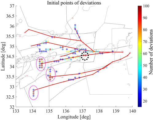
FIGURE 1. Initial deviation points for west arrivals.

2.2 The Nagel–Schreckenberg cellular automata and its Relevance to the current research

This research is inspired by cellular automata (CA), in particular the Nagel–Schreckenberg (NS) model l (Nagel and Schreckenberg, 1992). Using CA, airspace can be coarse-grained into cells, with each cell having two discrete states-either empty or occupied by an aircraft. In CA, time advances with discrete steps. At each time step, the progress of each aircraft, i.e., how many cells it will go forward, is updated based on the neighboring cells’ availability and position updating rules. Aircraft movement properties like constant speed movement, acceleration and crash avoidance can all be modeled with the appropriate speed decision algorithm. The most well-known application of CA to traffic modeling is in ground traffic simulations. Merging lanes aside, in the spatial domain these simulations are often one-dimensional- the vehicle can either stop or proceed to the next cell towards its destination. There are multiple applications of cellular automata to ground taxiing modeling (Mori, 2012; Mazur and Schreckenberg, 2018). In the case of airborne air traffic however, and terminal area air traffic in particular, such modeling is not straightforward, as a lot of vectoring, or path stretching in the lateral plane exists. In other words, aircraft do not follow their planned route, but are often deviated in the lateral direction by ATC so that the necessary separation requirements are met. This can be seen from sample tracks for Hiroshima-Tokyo International (Haneda) flights from a week of July 2019, as shown in Figure 2. The published route is shown in red, and the actual lateral trajectories are shown in blue. To overcome this major obstacle, this study proposes mapping of each actual track data set (actual flight trajectory, available from CARATS Open Data, published by Japan Civil Aviation Bureau) on the nominal route determined by the departure-arrival airport pair. The nominal route data is obtained from Japan Aeronautical Information Service Center database (Ministry of Land, 2019). Past research proposed mapping on the most common route found in a specific data set (Andreeva-Mori, 2021), but discussions with pilots and air traffic controllers suggested the use of nominal routes instead.

FIGURE 2

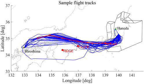
FIGURE 2. Lateral tracks of Hiroshima-Haneda flights on a week of July 2019.

Once the routes which are analogous to roads for the ground traffic are determined, these routes need to be discretized in cells so that the aircraft proceeds a certain number of cells at each step. The size of the cells is optimized so that non-vectored flights, i.e., flights with trajectories which are close to the nominal routes and experienced neither path stretching nor short-cuts, proceed 1 cell at a time. This size optimization is important for the CA, as it helps derive simple rules, thus allowing to model complicated interactions later and also aids explainability.

The CA-inspired analysis of air traffic is performed following the steps below:

1 Identify and select city-pair routes in analogy to roads in the CA model.

2 Use real past radar data to identify the right size of the cell (cf. velocity in the CA model)—the main assumption being that nominal flights, i.e., flights which experience little interference from other traffic should move 1 cell every time unit.

3 Model the movements of non-nominal flights based on the nominal route and cell size assumptions established in steps 1 and 2. The trajectory of each flight is mapped on its nominal route. Consider a sample flight (blue) and basic route (grey cells) as the ones shown in Figure 3.Assume trajectory data is available every 10 s. Each of the data points in the original trajectory is mapped to the nominal route, either using the shortest distance or any other projection algorithm. Assume for each trajectory point i, the distance between this point and each cell of the basic route is calculated. Trajectory point i is then mapped to the closest cell determined by the minimum distance. For example, in the trajectory sample shown in Figure 3, point i = 3 is closest to cell #2, so it is mapped there. Iterating this process over all trajectory points creates mapping [1 2 2 3 3 4 5 6 7 8 8 9 10 10 11 12]. The example presented here uses closest distance to map the trajectory to the basic route, but other mapping algorithms are also possible, as discussed later in this research.

4 Analyze the mapped velocities of each flight and the entire traffic flow, and propose a metric to characterize the traffic on each day.

FIGURE 3

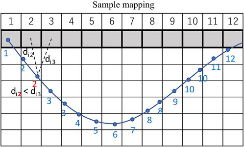
FIGURE 3. Trajectory mapping concept.

3 Mapping

3.1 Flight radar data

Analysis in this research is based on CARATS Open Data (July 2019- March 2020), route surveillance radar flight track data released by Japan Civil Aviation Bureau (Oka, 2019). Data is available for a week of flights every month, i.e., altogether 12 weeks of data per year, for about 4000 flights per day on average. The radar data for each flight consists of pseudo flight number, aircraft type, as well as latitude, longitude and altitude data recorded every 10 s, on average.

3.2 Selection of nominal routes

In the case of ground traffic, vehicles follow roads, so their movement is limited by the road network. In the case of air traffic, however, even though air routes still exist, many flights experience shortcuts or path stretching so that safe spacing with other traffic is maintained. Early research considered defining the routes based on the track data only, by identifying the routes which were most commonly used (Andreeva-Mori, 2021). The major disadvantage of this approach is the lack of consistency and explainability. Alternatively, using flight plans would be ideal, but since these are not available, this research opts for published routes. Each flight plan can be divided into three main parts-departure, enroute and arrival. Each flight to be operated under instrument flight rules (IFR) files a flight plan containing information on all three phases. The enroute plan is based on routes published in the relevant enroute charts for the airspace which is used, and consists of a list of navigational fixes (waypoints and intersections) connected by published routes. The route depends on the city pair, but similar to ground traffic, there might be more than a single option and the particular enroute choice depends on the airline, weather and traffic. This research uses information published in AIS Japan as of June 2019 (Ministry of Land, Infrastructure, Transport and Tourism n.d.). This research is focused on Tokyo International (Haneda) Airport west arrivals, which under north wind conditions land at runway 34L. The portion of the flight from take-off until the first enroute point is described by a set of flight legs referred to as a standard instrument departure (SID) and a transition. In most cases, each airport has multiple SIDs and the one to be used by each flight depends on the runway configuration, weather conditions, noise restrictions and interference with other traffic (Heffar et al., 2021). Similarly, a standard terminal arrival route (STAR) connects the last waypoint of the enroute to the first waypoint of the final approach to the arrival airport. Flights arriving at Haneda Airport Runway 34L enter Tokyo Approach Control Area (Tokyo ACA) at 5 waypoints- SPENS, SELNO, TOPIT, DOLBA and LALID. TOPIT is used by flights coming from Hachijojima, a small island on the south of Tokyo, whereas DOLBA and LALID are mainly used by international flights coming from North America. These three waypoints combined are used by a limited number of flights every day, so this research focuses only on SPENS and SELNO arrivals. Furthermore, the current analysis is limited to the area 150 NM from Haneda Airport, as shown in Figure 4. Haneda Airport introduced Point Merge System (PMS) in July 2019, making Haneda the 18th airport worldwide to adopt this arrivals sequencing method (EUROCONTROL, 2022; Supporting European Aviation, 2023). This research models traffic using PMS arrivals via OSHIMA (XAC) 1A/1K and AKSEL 1A/1K for SPENS and SELNO respectively.

FIGURE 4

FIGURE 4. PMS area, Tokyo Approach Control Area (ACA) and incoming flows.

3.3 Cell definition and sizing

The size of the cells is important to accurately analyze traffic flow and merges. In the traditional cellular automata, the vehicle proceeds 1 cell at a time when no other traffic interferences are present. If the cells are too big, the aircraft will stay in the same cell for multiple time units and jump to the next cell at once. On the other hand, if the cells are too small, the aircraft will move too many cells ahead at a time, which could unnecessarily complicate the model. The optimal cell size depends on the ground speed of the aircraft. Each flight reaches its maximum speed in the enroute phase, which is usually executed at a more or less constant speed. During the descent in the vicinity of Haneda Airport, the speed decreases. With proper rule definitions, various speeds can be modeled within CA even for vehicles not interfering with other traffic, but this complicates the model. This research defines the cell size so that non-vectored (nominal) flights proceed 1 cell per unit time (velocity is 1) regardless of their flight phase. The current analysis is based on the ground speed of the aircraft, but in reality wind conditions and different speed airspeed profiles can be reasons for non-vectored flights’ velocity to appear faster or slower than 1. For example, increasing the speed enroute to minimize the arrival delay to compensate for any accumulated delays from previous flights with the same aircraft on a single day is an illustration of this phenomenon. In this example, the flight will have a velocity larger than 1 even though it may be following the basic route. Another example is a flight on a day with strong tail wind. Similarly, in such a case the velocity will exceed 1 as well. The current investigation is an initial research on the potential of CA-based mapping to evaluate flight efficiency and does not model the above influences explicitly, as they are part of a follow-up publication. The data used in this paper, however, covers a wide range of meteorological conditions (July 2019 to March 2020), which helps us define an average cell size appropriate for the current investigation. Weather, in particular wind, will be modeled by adjusting the cell size for each day based on the meteorological data available. Wind data will be used to obtain null-wind simulated trajectory times, i.e., an estimation of the flight time had there been no wind, which will be used to calculate the optimal cell size. A similar approach was adopted in the author’s past work to estimate basic flight times (Andreeva-Mori and Onji, 2022).

To account for decelerations at arrival, 2 cell sizes are defined-enroute cell size, which is applied to the phase from 150 NM our of Haneda Airport to Tokyo ACA area entry waypoints (either SPENS or SELNO), and the transition phase, applied from SPENS/SELNO to the first waypoint in the arc-shaped route of the PMS. Analysis results conducted for the data available from July 2019 to March 2020 focusing on the lateral distance between the top of descent (ToD, i.e., the end of the enroute phase) and Tokyo ACA entry fix are shown in the histogram in Figure 5. This distance is assumed positive when ToD is prior to Tokyo ACA entry fix and negative otherwise. As seen from the histogram, 97.4% of the flights have started descent prior to entering Tokyo ACA. This figure does not vary much among the two major fixes either-it stands at 97.5% for SPENS and 98.3%. The above results show that for SPENS and SELNO fixes more than 97% of RWY34L arrivals cross these entry fixes after the completion of the enroute phase. Note, however, that there is a significant variation in the position of the ToD so this is expected to cause variations in the velocities when the traffic is modeled by constant-size cells.

FIGURE 5

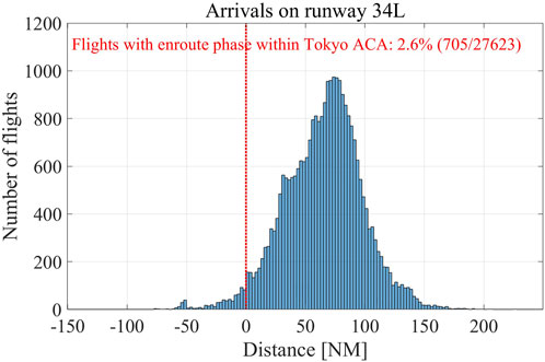
FIGURE 5. Distance between the Top of Descent and Tokyo ACA entry points for Runway 34L arrivals.

The flight radar data is available every 10 s on average. The cell sizes for both the enroute and transition areas are determined so that non-vectored flights proceed 1 cell at every time step, i.e., every 10 s. First, the original flight radar data is pre-processed to create data with one data point every 10 s. Second, the deviation from the nominal route is calculated. Next, based on the calculated deviation non-vectored flights are selected. Finally, these are used to define the cell size in each phase, enroute and transitional. The data pre-processing makes two corrections to the original data-first, the initial trajectory point is interpolated so that it coincides exactly with the 150 NM border of the target airspace, and second, the time interval between every two data points is adjusted to 10 s exactly. Deviations from the nominal route are calculated after the original lateral trajectories are mapped on the corresponding nominal route. Two mapping methods are considered- 1) mapping perpendicular to the flight leg of the nominal route, and 2) mapping parallel to the meridian. In the case of mapping method 1), some portions of the trajectory near the end of the flight legs are often mapped incorrectly (see Panel (a) of Figure 6), so in this paper mapping method 2) is used. The data points of the trajectory subject to mapping are defined as follows-the enroute mapping starts from the point nearest to the 150 NM border an ends with the point which longitude does not exceed the longitude of the corresponding Tokyo ACA entry fix (either SPENS or SELNO); the transitional mapping starts with the point following the last point of the enroute mapping and ends with the last point which longitude does not exceed the longitude of the last nominal route point. This is illustrated in Panel (b) of Figure 6. Once all trajectories are mapped, the distance between each point between the original trajectory point and its projection on the nominal route is calculated. When the deviation is less than 1 NM for 95% of all data points in the phase (either enroute or transitional), the flight is considered non-vectored, or unimpeded. The cell size for both phases for both SPENS and SELNO streams is determined so that non-vectored flights’ velocity is 1 cell per 10 s.

FIGURE 6

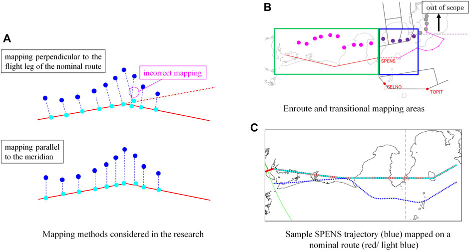
FIGURE 6. Mapping methods and areas. (A) Mapping methods considered. (B) Enroute and transitional mapping areas. (C) Sample trajectory mapping.

From all flights on SPENS routes, 726 meet the non-vectored requirements in the enroute phase and 3008 in the transitional phase. The lateral flight distances over each step for these flights are summarized in the histograms in the left panel of Figure 7. For SELNO flights, there are 58 non-vectored enroute flights and 238 non-vectored transitional flights. The flight distances over each 10 s are shown in the right panel of Figure 7. The average values, highlighted in yellow, are selected as cell sizes for each route. Note that in this paper velocity is used to describe the aircraft movement per unit time, in accordance with the language used in the Nagel–Schreckenberg (NS) Cellular Automata model.

FIGURE 7

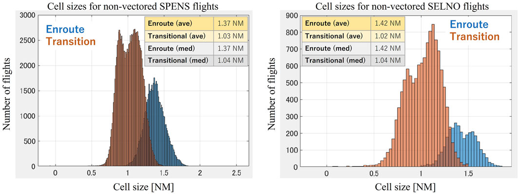
FIGURE 7. Cell sizes of non-vectored SPENS and SELNO flights.

4 Velocity analysis

4.1 Single flight analysis

The average velocities on each day of traffic for which more than 400 flights used runway 34 L for arrivals are calculated. The threshold used to differentiate impeded, or vectored flights, is defined as the 25th percentile of the mean velocities of all flights on that day, is determined for each day and shown in the histograms in Figure 8. Consider 12 Sep 2019 as a sample day of traffic. For this day, the velocity threshold at SPENS is 0.89. There were 279 flights arriving via SPENS on this day. The velocity profiles and original flight tracks of flight 51 to 78 are shown in Figure 9. The horizontal axis shows cell numbers and the vertical axis indicates velocity, i.e., cell movements per time step of 10 s. Slow flights with average velocity of less than the threshold of 0.89 cells/time step are shown in red. For the remaining flights, for the majority of the time they move at a velocity 1 cell/time step. Note that cell No.1 here is the first cell after the flight has entered the 150 NM area. The grey vertical line indicates the mapping at SPENS, which is the end of the enroute and the start of the transitional phase. The original trajectories are shown to verify the accuracy of the proposed analysis. As seen from the figure, the trajectories of most flights with near-1 velocity are almost non-vectored, whereas slow flights are characterized by significant path-stretching. The mean velocity of the flight can be used as an efficiency and traffic impediment metric.

FIGURE 8

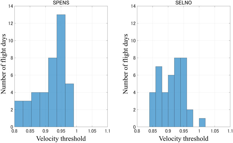
FIGURE 8. Velocity histograms.

FIGURE 9

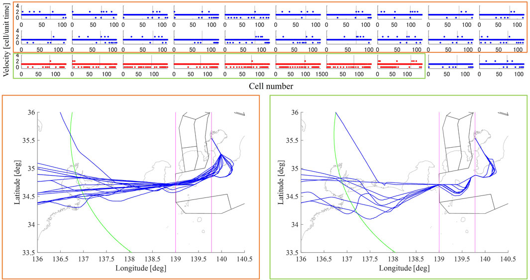
FIGURE 9. Velocity profiles and lateral tracks for non-vectored (orange) and vectored (green) flights. Upper panel: the horizontal axis shows time, vertical axis shows cell movements per unit time, i.e., velocity. Lower panels: lateral tracks of the corresponding flights.

4.2 Multiple flight velocity analysis

4.2.1 Full traffic space-time diagrams

The traffic on each day can be visualized by time-space diagrams such as the one in Figure 10. The vertical axis shows the time, and the horizontal one shows the cell number, with Cell 0 being the final cell of the transitional phase. Note that due to the different length of nominal routes and the definition of the first enroute data point to be mapped (see Section 3.3), the initial point varies for each flight. Unimpeded flights proceed 1 cell per unit time. Short-cuts/accelerations are expressed as “skipped cells,” and vectoring/decelerations are shown as vertical line segments. SPENS arrivals are shown in blue, and SELNO arrivals are shown in light green. The distance in cells to the preceding flight can be calculated from the horizonal axis at any given time. A sample diagram for the traffic on 14 September 2019, 16:40-17:00 is shown in Figure 10. “A” denotes SPENS flights, and “B” denotes SELNO flights. For example, at 16:40, flights 3A and 4A are 12 cells apart and this separation is more or less maintained until they reach Cell 0. On the other hand, at 16:40 flights 7A and 8A, both arriving via SPENS, are only 5 cells apart, but at 16:52 they are already 11 cells apart. In this interval, flight 8A has zero velocity at 10 cells and velocity of 2 once, whereas flight 7A has zero velocity at 6 cells and velocity of 2 at 2 cells, which results in increased separation. Furthermore, for these two flights in particular, the adjustments seem to have been made prior to cell 35. Note that for most flights the enroute phase ends between cells 40 and 50, so these results indicate that ATCo have spaced these two flights before they crossed SPENS, i.e., prior to their entering Tokyo ACA. This is clearly not the case for flights from different flows, as seen for the case of flights 9A, 2B, and 3B. Both SELNO flights, 2B and 3B are only 3 cells apart at 16:40 and maintain more or less the same small separation until 16:48, when one of the flights is gradually slowed down to provide increased separation which reaches 12 cells at 16:56. At this time, however, the SPENS flight 9A and SELNO flight 3B are only 1 cell apart, which indicates that ATCo have not considered merging SELNO and SPENS traffic yet.

FIGURE 10

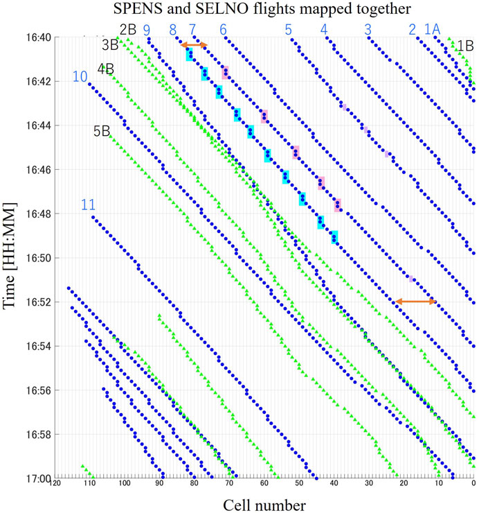
FIGURE 10. A sample time-space diagram for the traffic on 14 Sep 2019, 16:40-17:00.

4.2.2 Deceleration analysis

Similar to the single lane Nagel–Schreckenberg cellular automata, the example above demonstrates that deceleration depends on the number of cells to the preceding aircraft. The main difference between the current mapping and the NS model is that the physical location of a cell i on each of the SPENS and SELNO routes might differ, as these include several branches which were not modelled individually. Furthermore, the current mapping represents dimensionally reduced vectored trajectories, which were originally laterally deconflicted. Therefore, strictly speaking, aircraft can be in the same or a nearby cell at the same time on a single stream and not violate the safety separation standards.

The velocity profiles of all flights can be used to generate an overall ground speed distribution over all cells. The average velocities for four sample days are shown in Figure 11. Note that cell zero is the one at the end of the mapping range and closest to the arrival airport. The red line indicates the median location of the transition fix for each flight, and the blue rectangle shows the 25th and 75th percentile of the locations. For example, on 11 November 2019 most flights transitioned at cell No. 69, and half of all flights transitioned between cell No. 58 and 76. Note that the cell size changes after the transition, as indicated in Figure 7. The grey-shaded area in the left of the figures indicate areas with a small amount of data, so the sudden dive should be disregarded. The average velocities depend greatly on the cell number. The velocity is more or less stable between cells 120 and 60, with some days (November 11 and December 09) experiencing more fluctuations than others. It drops after that, but this may be partly due to the change in the cell size as well. The drop, however, does not happen right after the transition point, so it could be said that at least some of the decelerations after cell 60 and prior to cell 40 are due to ATC interventions. These results agree with the results from the initial analysis presented in Section 2 as well. The velocity increases at cell 40, which is the area near OSHIMA on the SPENS stream and gradually decreases after this. This velocity analysis indicates that ATCs merge traffic and make separation adjustments at two main areas-prior to entering Tokyo ACA and shortly after this entry. This operation style is reflecting the current airspace structure and indicates the potential for improvement towards seamless ATM.

FIGURE 11

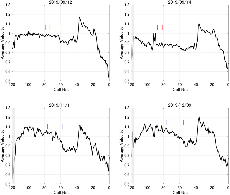
FIGURE 11. Sample average velocity profiles.

Analysis of the velocity versus the distance between the aircraft and the preceding one is conducted using the proposed mapping. Note that as in the time-space graph presented in the previous section, a velocity of 1 cell is the nominal one, velocity of zero indicates deceleration, and velocities of 2 and higher indicate acceleration. Sample results for September 12 and November 12 are shown in Figure 12. Note that the number of flights on both days are almost the same- 401 (279 via SPENS and 122 via SELNO) flights on September 12, and 406 (275 via SPENS and 131 via SELNO) flights on November 12. Boxplots are drawn based on the entire dataset and each SPENS and SELNO subsets. The red line in the middle of each box is the median, and the bottom and top of each box (shown in blue) are the 25th and 75th percentiles, respectively. Outliers are shown in red. The confidence interval is shown by the notch. Note that in all cases, the velocity increases as the number of empty cells ahead increases. Since the data includes non-congested times like early mornings, for example, some of the outliers have very high values reaching 100 cells, which exceeds 16 min of separation. Analysis of the single flows through SPENS and SELNO shows that the distance to the preceding aircraft is generally larger in the SELNO stream, but this is partly due to the smaller number of aircraft in this stream. The medians for the velocity = 1 group are 11 cells for SPENS and 19 for SELNO on September 12, and 13 cells for SPENS and 21 for SELNO on Nov12. The medians for the velocity = 0 group, which corresponds to deceleration, or vectoring, are 9 cells for SPENS and 13 for SELNO on September 12, and 8 cells for SPENS and 14 for SELNO on Nov12. Similarly, the medians for the acceleration case expressed by velocity = 2, are 13.5 cells for SPENS and 20 for SELNO on September 12, and 17 cells for SPENS and 25 for SELNO on Nov12. Note that on November 12 some flights had negative velocity, which means they moved back a cell (velocity = −1) or two (velocity = −2). These are irregular traffic flow cases, which describe holding patterns, for example.

FIGURE 12

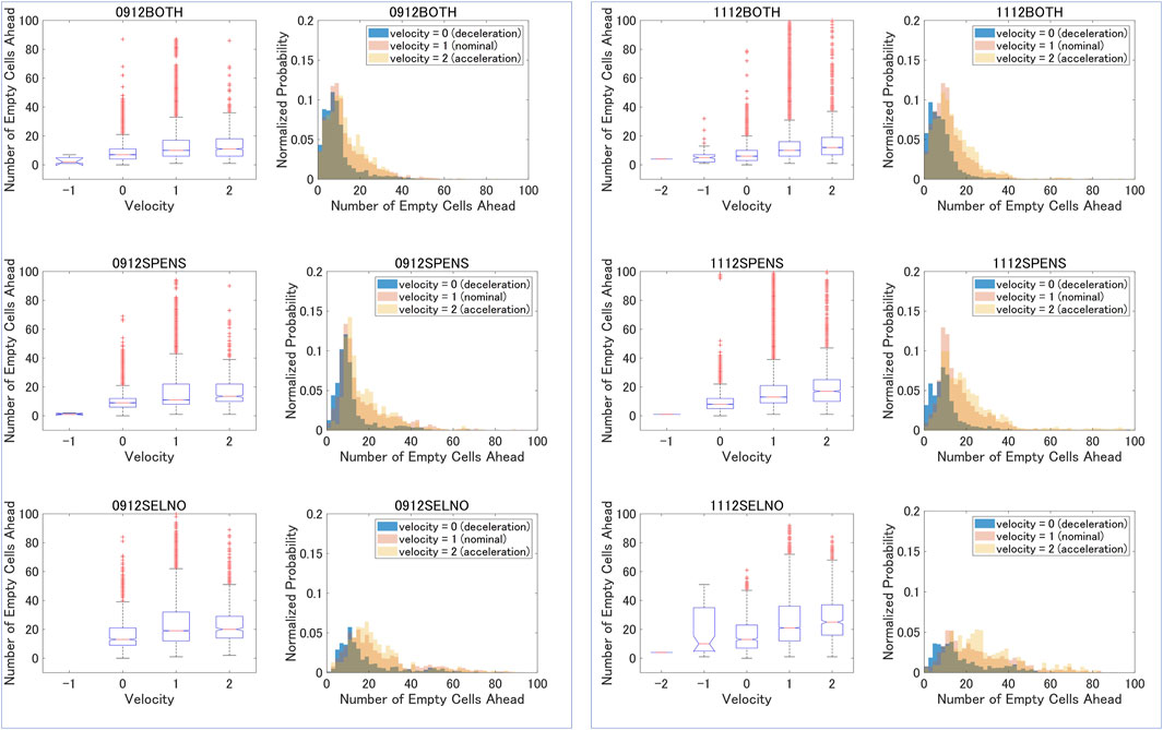
FIGURE 12. Dependency of the velocity on the number of empty cells ahead.

The histograms on the right of the boxplots illustrate the distributions which can be used to describe each of the velocities. The histogram of velocity 0 is shifted to the left of the nominal histogram (velocity 1) and the histogram of velocity 2 is shifted to the right of the nominal one, which indicates that deceleration occurs when the distance to the preceding flight is smaller than the nominal one, and acceleration occurs when more empty cells are available ahead.

Each flight can be described by the number of cells with velocities equal to −2, −1, 0, 1, and 2. A flight with a large number of cells with velocity 1 is one which performs close to the original route and is very predictable, a valuable characteristic for time-based air traffic management. Furthermore, for each day the percentage of cells with corresponding velocities equal to −2, −1, 0, 1, and 2 can be determined. The results of the traffic for 52 sample days are shown in Figure 13. The nominal velocity of 1 is predominant on all days, but the percentage varies between 78% and 88%. Velocity of 1 provides a high predictability of the trajectory and in the context of overall traffic flow control and time-based flow management is preferable. On the contrary, velocity of 0 occurs between 6% and 16% for the sample data set. Note that the day with minimum value for cells with velocity 0 experiences the maximum value for velocity 2, i.e., many flights were able to fly shorter routes than the nominal ones. Most days are characterised by very small values for cells with negative velocities. There are three notable exceptions, i.e., pseudo day No. 7, 18, and 39, when more than 1.4% of the cells had negative velocities. The disturbances in the traffic on those 3 days seem more significant, and this is supported by the lateral trajectories of the flights as well. A sample of 12 flights which were put into holding patterns on pseudo day 18 are shown in Figure 14.

FIGURE 13

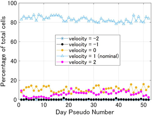
FIGURE 13. Velocity distributions over 52 sample days.

FIGURE 14

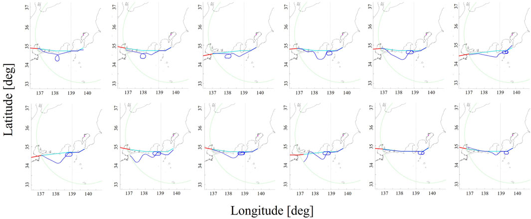
FIGURE 14. Several lateral trajectory profiles from pseudo day No. 18.

5 Discussion on potential applications

The proposed mapping, and the velocity-cell analysis in particular, can be used to reveal where ATC intervenes to merge and separate traffic, and evaluate how close the operations are to the seamless ATM, promoted by ICAO and aimed to ensure safe and efficient air transport (International Civil Aviation Organization ICAO, 2019). The correlation between velocity and empty cells ahead can be further quantified by distribution models and applied to real traffic modeling based on cellular automata. A major application of the proposed mapping is traffic inefficiency and predictability evaluation. Orderly and predictable traffic is described by velocity 1 cell/unit time over all cells and times. Traditional path stretching or vectoring is described by velocity 0 cell/unit time, holding is expressed by fluctuating negative and positive velocity patterns, and direct routes and accelerations are mapped by velocity of 2 or higher. Assigning relative weights to each of these characteristics and summing over all flights results in a traffic metric, as shown in Eq. 1 below.

$TrafficMetric={\displaystyle {\sum }_{i=i_{\mathit{min}}}^{i_{\mathit{max}}}}{w}_i{v}_i(1)$

In the metric above, $w_i$ are the weights assigned to each velocity and $v_i$ is the relative percentage of cells with speed $i$ over the target spatial and temporal mapping interval. Assume large values of the metric are better than small ones, and one wishes to prioritize predictability. In such a case, the highest weight should be assigned to $w_1$. If time is prioritized, then shortcuts will be evaluated higher, so $w_{i\ge 2}$ will be of the largest values. Holding patterns and vectoring can be evaluated separately by assigning different values for $w_{i\le -1}$ and $w_0$. The most significant advantage of the proposed metric is that it can capture both the spatial and temporal traffic characteristics, and is simple to calculate based on track data and published routes only.

6 Concluding remarks

This research introduced how a discrete and spatial mapping inspired from cellular automata can be used to evaluate air traffic predictability and inefficiencies. Unveiling where, when, and what type of inefficiencies occur can benefit post-operational analysis and provide insight into potential improvements. A traffic metric adjustable to the stakeholder’s needs, for example, focusing on either traffic predictability, key for trajectory-based operations, or flight efficiency, essential for sustainable traffic was also proposed. The results from the research can be further expanded to investigate the correlation between adverse-weather and traffic inefficiencies, but the current work provides the necessary platform for such analysis and is therefore considered beneficial to inform the relevant stakeholders.

Data availability statement

The data analyzed in this study is subject to the following licenses/restrictions: CARATS Open Data released by Japan Civil Aviation Bureau was used in the current analysis. Requests to access these datasets should be directed to https://www.mlit.go.jp/koku/koku_fr13_000006.html.

Author contributions

AA-M: Conceptualization, Formal Analysis, Funding acquisition, Investigation, Methodology, Validation, Writing–original draft, Writing–review and editing.

Funding

The author(s) declare financial support was received for the research, authorship, and/or publication of this article. This work was supported by JSPS KAKENHI “Heterogeneous air traffic flow modeling and congestion mechanism clarification,” Grant Number 20K14855.

Acknowledgments

The author is grateful to Japan Civil Aviation Bureau and the CARATS Open Data initiative though which the flight track data was obtained. The author would like to thank colleagues in the Smart Flight team and Dr. Seiya Ueno in particular for insightful comments and advice.

Conflict of interest

The author declares that the research was conducted in the absence of any commercial or financial relationships that could be construed as a potential conflict of interest.

Publisher’s note

All claims expressed in this article are solely those of the authors and do not necessarily represent those of their affiliated organizations, or those of the publisher, the editors and the reviewers. Any product that may be evaluated in this article, or claim that may be made by its manufacturer, is not guaranteed or endorsed by the publisher.

References

Airbus (1998). Getting to grips with the cost index. Available at: https://ansperformance.eu/library/airbus-cost-index.pdf (Accessed November 29, 2023).

Google Scholar

Andreeva-Mori, A. (2021). Preliminary parameter investigation for cellular automata air traffic flow modelling. AIAA Aviat., 3012. 2021 Forum. Virtual. doi:10.2514/6.2021-3012

CrossRef Full Text | Google Scholar

Andreeva-Mori, A., and Onji, M. (2022). “Dynamic airborne delay buffer selection for efficient air traffic flow management,” in Proceedings of International Workshop on ATM/CNS 2022 International Workshop on ATM/CNS, Tokyo.

Google Scholar

Bayen, A. M., Raffard, R. L., and Tomlin, C. J. (2006). Adjoint-based control of a new eulerian network model of air traffic flow. IEEE Trans. Control Syst. Technol. 14 (5), 804–818. doi:10.1109/tcst.2006.876904

CrossRef Full Text | Google Scholar

CANSO (2023). Recommended key performance indicators for measuring ANSP operational performance. Available at: https://canso.org/publication/recommended-key-performance-indicators-for-measuring-ansp-operational-performance/(Accessed November 29, 2023).

Google Scholar

EUROCONTROL (2022). Performance review report (PRR) 2022.

Google Scholar

EUROCONTROL/FAA (2013). 2012ComparisonofAirTraffic management-related operational performance: US/europe.

Google Scholar

Heffar, A., Dalmau, R., and Allard, E. (2021). Prediction of flight departure and arrival routes with gradient boosted decision trees. 11th SESAR Innovation Days.

Google Scholar

International Civil Aviation Organization (2009). ICAO manual on global performance of the air navigation system. ICAO. Doc 9883.

Google Scholar

International Civil Aviation Organization (ICAO) (2019). Asia/pacific seamless ANS plan V3.0.

Google Scholar

Kuljanin, J., Pons-Prats, J., and Prats, X. (2021). “Fuel-based flight inefficiency through the lens of different airlines and route characteristics,” in Fourteenth USA/europe air traffic management research and development seminar.

Google Scholar

Lemetti, A., Hardell, H., and Polishchuk, T. (2023). Arrival flight efficiency in pre- and post-Covid-19 pandemics. J. Air Transp. Manag. 107, 102327. doi:10.1016/j.jairtraman.2022.102327

PubMed Abstract | CrossRef Full Text | Google Scholar

Liu, Y., Hansen, M., Ball, M. O., and Lovell, D. J. (2021). Causal analysis of flight en route inefficiency. Transp. Res. Part B Methodol. 151, 91–115. doi:10.1016/j.trb.2021.07.003

CrossRef Full Text | Google Scholar

Mazur, F., and Schreckenberg, M. (2018). Simulation and optimization of ground traffic on airports using cellular automata. Collect. Dyn. 3, A14–A22. doi:10.17815/cd.2018.14

CrossRef Full Text | Google Scholar

McKinsey&Company (2023). Decarbonizing aviation: executing on net-zero goals. 06 16Available at: https://www.mckinsey.com/industries/aerospace-and-defense/our-insights/decarbonizing-aviation-executing-on-net-zero-goals (Accessed January 26, 2024).

Google Scholar

Ministry of Land (2019). Infrastructure, transport and tourism. AIS Japan. Available at: https://aisjapan.mlit.go.jp/Login.do. [Accessed 15 February (June 19, 2019).

Google Scholar

Mori, R. (2012). Aircraft ground-taxiing model for congested airport using cellular automata. IEEE Trans. Intelligent Transp. Syst. 14 (1), 180–188. doi:10.1109/tits.2012.2208188

CrossRef Full Text | Google Scholar

Nagel, K., and Schreckenberg, M. (1992). A cellular automaton model for freeway traffic. J. de physique I 2 (12), 2221–2229. doi:10.1051/jp1:1992277

CrossRef Full Text | Google Scholar

Oka, M. (2019). CARATS open data- explanations (in Japanese). 8 7. Available at: http://www.mlit.go.jp/common/001231892.pdf.

Google Scholar

Prats, X., Dalmau, R., and Barrado, C. (2019). “Identifying the sources of flight inefficiency from historical aircraft trajectories,” in Thirteenth USA/Europe air traffic management research and development seminar (London, UK).

Google Scholar

Prats, X., Barrado, C., Netjasov, F., Crnogorac, D., Pavlovic, G., Agüi, I., et al. (2018). Enhanced indicators to monitor ATM performance in Europe. SESAR Innov. Days, 90.

Google Scholar

Reynolds, T. G. (2014). Air traffic management performance assessment using flight inefficiency metrics. Transp. Policy 34, 63–74. doi:10.1016/j.tranpol.2014.02.019

CrossRef Full Text | Google Scholar

Sridhar, B., Soni, T., Sheth, K., and Gano, B. (2006). Aggregate flow model for air-traffic management. J. Guid. Control, Dyn. 29 (4), 992–997. doi:10.2514/1.10989

CrossRef Full Text | Google Scholar

Supporting European Aviation (2023). Tokyo-Haneda, one of the world’s busiest airports, set to implement Point Merge, EUROCONTROL’s innovative method for sequencing arrival flows. Available at: https://www.eurocontrol.int/news/tokyo-haneda-one-worlds-busiest-airports-set-implement-point-merge-eurocontrols-innovative (Accessed April 10, 2023).

Google Scholar