Deep-Learning Computational Holography: A Review

1 Introduction

Holography (Gabor, 1948) can record three-dimensional (3D) information of light waves on a two-dimensional (2D) hologram as well as reproduce the 3D information from the hologram. Computer-generated holograms and holographic 3D measurements (digital holography) can be realized by simulating this physical process on a computer. Computer-generated holograms can be generated by calculating light wave propagation (diffraction) emitted from 3D objects. If this hologram is displayed on a spatial light modulator (SLM), the 3D image can be reproduced in space. Holographic displays can successfully reproduce the wavefront of 3D objects, making them ideal 3D displays (Hilaire et al., 1990; Takaki and Okada, 2009; Chang et al., 2020).

In contrast, digital holography (Goodman and Lawrence, 1967; Kim, 2010; Liu et al., 2018; Tahara et al., 2018) is a technique that uses an image sensor to capture a hologram of real macroscale objects or cells. Diffraction calculations are used to obtain numerically reproduced images from the hologram. Digital holography has been the subject of much research in 3D sensing and microscopy. In addition to coherent light, the technique of capturing holograms with incoherent light has been actively studied in recent years (Liu et al., 2018; Rosen et al., 2019).

Computational holography is the general term for handling holography on a computer. It has been widely used in 3D display, projection, measurement, optical cryptography, and memory. The following are common problems of computational holography that need to be addressed:

(1) A high computational complexity for hologram and diffraction calculations.

(2) A limited image quality of the reproduced images from holograms, due to speckle noise, optical abberations, etc.

(3) A large amount of data required to store holograms.

The computational complexity of hologram calculations increases with the complexity of 3D objects and the resolution of a hologram. Digital holography requires diffraction calculations to obtain the complex amplitude of object light, followed by aberration correction of the optical system, and phase unwrapping, if necessary. Additionally, autofocusing using an object position prediction may be necessary. These are time-consuming calculations.

The quality of the reproduced images from a hologram is also a critical issue in holographic displays and digital holography. The following factors degrade reproduced images: high-order diffracted light due to the pixel structure of SLMs, quantized and non-linear light modulation of SLMs, alignment accuracy, and aberration of optical systems.

The amount of data in holograms is also a major problem. Data compression is essential for real-time hologram transmission and wide-viewing-angle holographic displays, which require holograms with a large spatial bandwidth product (Blinder et al., 2019). Hologram compression using existing data compression methods, such as JPEG and JPEG2000, and original compression methods for hologram have been investigated (Blinder et al., 2014; Birnbaum et al., 2019; Stepien et al., 2020) and recently the JPEG committee (ISO/IEC JTC 1/SC 29/WG 1) initated the standardization of compression technology for holographic data.

Many studies have developed algorithms based on the physical phenomena of holography (diffraction and interference of light) and signal processing. In this paper, we refer to these algorithms as physically-based calculation. In 2012, AlexNet (Krizhevsky et al., 2012), which uses deep neural networks (DNNs), achieved an improvement of more than 10% over conventional methods in the ImageNet large-scale visual recognition challenge, a competition for object recognition rates. This led to a great deal of interest in deep learning (LeCun et al., 2015). In 2017, research using deep learning started increasing in computational holography. Initially, simple problems using deep learning, such as the hologram identification problem and restoration of holographic reproduced images, were investigated (Shimobaba et al., 2017a; Shimobaba et al., 2017b; Jo et al., 2017; Muramatsu et al., 2017; Pitkäaho et al., 2017). Currently, more complex deep-learning-based algorithms have been developed, and many results have been reported that outperform physically-based calculations.

This review presents an overview of deep-learning-based computer-generated hologram and digital holography. In addition, we outline diffractive neural networks, which are closely related to holography. It is worth noting that deep learning outperforms conventional physically-based calculations in terms of computational speed and image quality in several holographic applications. Additionally, deep learning has led to the development of techniques for inter-converting images captured by digital holographic and other microscopes, blurring the boundaries between research areas. Furthermore, we will discuss our personal views on the relationship between physically-based calculations and deep learning in the future.

2 Hologram Computation Using Deep Learning

Computer-generated holography has many applications, such as 3D display (Hilaire et al., 1990; Takaki and Okada, 2009; Chang et al., 2020), projection (Buckley, 2011; Makowski et al., 2012), beam generation (Yao and Padgett, 2011), and laser processing (Hasegawa et al., 2006). This section focuses on hologram calculations for holographic display applications.

Figure 1 shows the data processing pipeline of holographic displays. From 3D data, acquired using computer graphics and 3D cameras, the distribution of light waves on a hologram is calculated using diffraction theory. The generated hologram is usually complex-valued data (complex holograms); however, SLMs can only modulate amplitude or phase. Therefore, we must encode the complex hologram into amplitude or phase-only holograms. The encoded hologram can be displayed on the SLM and the 3D image can be observed through the optical system.

FIGURE 1

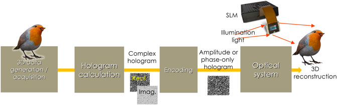
FIGURE 1. Data processing pipeline for holographic displays.

The 3D data format handled in physically-based hologram calculations can be classified into four main categories: point cloud (Lucente, 1993; Yamaguchi et al., 1993; Kang et al., 2008; Shimobaba et al., 2009; Hiroshi Yoshikawa and Yoshikawa, 2011; Blinder and Schelkens, 2020), polygon (Ahrenberg et al., 2008; Matsushima and Nakahara, 2009; Zhang et al., 2018a), layered (RGBD images) (Okada et al., 2013; Chen et al., 2014; Chen and Chu, 2015; Zhao et al., 2015), and light field (multiviewpoint images) (Yatagai, 1976; Zhang et al., 2015). Fast computation methods for each 3D data format have been proposed (Shimobaba et al., 2015; Nishitsuji et al., 2017; Tsang et al., 2018; Blinder et al., 2019). For the hologram computation using deep learning, some research has been conducted on the point cloud method (Kang et al., 2021). However, the layer method has been the focus of research using deep learning. To the best of our knowledge, polygon and light-field methods using deep learning have not been investigated yet.

2.1 Supervised Learning

In 1998, hologram generation using a neural network with three fully-connected layers was investigated (Yamauchi et al., 1998). However, this is not deep learning, but it is similar to current deep-learning-based hologram calculations. To the best of our knowledge, this is the pioneering work using neural networks for hologram computation. It performed end-to-end learning to train the neural network using a dataset consisting of 16 × 16-pixel input images and holograms. The end-to-end learning method is a supervised learning technique and allows a DNN to learn physical processes used in physically-based calculations from a dataset alone. This study showed that the neural network could optimize holograms faster than direct binary search (Seldowitz et al., 1987). It was impossible to adopt the current deep network structure due to poor computing resources. Additionally, even if DNN could be created, there was no algorithm (optimizer) to optimize its large number of parameters. For a while, neural networks were not the mainstream in hologram calculation, and physically-based calculations were actively studied. However, since 2018, hologram calculations have developed rapidly using deep learning.

Figure 2 shows the DNN-based hologram computation using supervised learning. Horisaki et al. (2018) designed a DNN that directly infers holograms from input 2D images using end-to-end learning. For end-to-end learning, it is necessary to prepare a large dataset of input images $\mathcal{X}$ and their holograms $\mathcal{Y}$. DNNs can be represented as an arbitrary function by combining convolutional and other layers with nonlinear activation functions. In this paper, a DNN function is represented as $\mathcal{N}(\mathcal{X};\mathrm{\Theta })$, where Θ are the network parameters. The parameters Θ of the DNN in Horisaki et al. (2018) are updated by solving the minimization problem:

$\underset{\mathrm{\Theta }}{\text{minimize}}\mathcal{L}\left(\mathcal{N}\left(\mathcal{X};\mathrm{\Theta }\right),\mathcal{Y}\right),(1)$

where $\mathcal{L}$ is the loss function for calculating the error between the predicted hologram output from the DNN $(\mathcal{N}(\mathcal{X};\mathrm{\Theta }))$ and the ground-truth hologram $(\mathcal{Y})$. This DNN can infer a hologram from a 64 × 64-pixel 2D image several times faster, and the image quality is the same as obtained with the Gerchberg–Saxton (GS) algorithm (Gerchberg, 1972; FienupFienup, 1982).

FIGURE 2

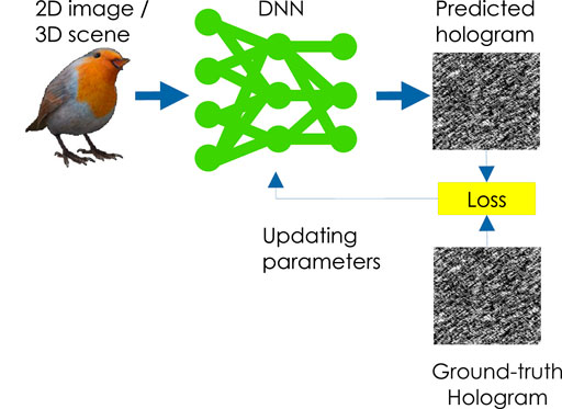
FIGURE 2. Deep neural network-based hologram computation using supervised learning.

Goi et al. (2020) proposed a method for generating binary holograms from 2D images directly using DNN. This study prepared a dataset of binary random patterns (binary holograms) and its reproduced images (original objects). The DNN was trained using end-to-end learning with the reproduced images as input of the DNN and the binary holograms as output. The output layer of the DNN should be a step function since it should be able to output binary values; however, this is not differentiable. The study Goi et al. (2020) used a differentiable activation function that approximates the step function.

2.2 Unsupervised Training

Unsupervised learning does not require the preparation of a dataset consisting of original images and its holograms, as discussed in Section 2.1. Figure 3 shows the DNN-based hologram calculation using unsupervised learning (Hossein Eybposh et al., 2020; Horisaki et al., 2021; Wu et al., 2021). We input the original 3D scene (or 2D image) $\mathcal{X}$ into the DNN and compute an inverse diffraction calculation (${\mathcal{P}}^{-1}$) from the predicted hologram to the location of the original object to obtain the reproduced image. We calculate a loss function between the reproduced image and the original data. Then, we update the DNN parameters by solving the following minimization problem:

$\underset{\mathrm{\Theta }}{\text{minimize}}\mathcal{L}\left(|{\mathcal{P}}^{-1}\left(\mathcal{N}\left(\mathcal{X};\mathrm{\Theta }\right)\right)|,\mathcal{X}\right).(2)$

FIGURE 3

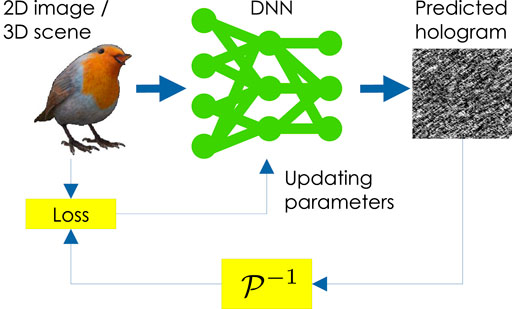
FIGURE 3. Deep neural network-based hologram calculation using unsupervised learning.

We can use any diffraction calculation for the propagation calculation, provided that it is differentiable. We usually use the angular spectrum method (Goodman and Goodman, 2005). The lightwave distribution on a plane u_d, which is z away from a plane u_s, can be calculated using the angular spectrum method expressed as follows:

$u_d=\mathcal{P}\left(u_s\right)={\mathcal{F}}^{-1}\left(\mathcal{F}\left(u_s\right)\exp \left(2\pi iz\sqrt{\frac{1}{{\mathrm{\lambda }}^2}-\left(f_x^2+f_y^2\right)}\right)\right),(3)$

where $i=\sqrt{-1}$, $\mathcal{F}$ and ${\mathcal{F}}^{-1}$ are the forward and inverse Fourier transforms, respectively; λ is the wavelength, and (f_x, f_y) represent the spatial frequencies.

Wu et al. (2021) showed that a hologram of a 4K 2D image could be generated in 0.15 s using unsupervised learning. The network structure of the issued DNN is U-Net (Ronneberger et al., 2015). Instead of the angular spectrum method, an inverse diffraction calculation to obtain the reproduced images was a single fast Fourier transform (FFT) Fresnel diffraction, which is computationally light. The DNN was trained using Eq. 2 a weighted combination of a negative Pearson correlation coefficient and a perceptual loss function (Johnson et al., 2016). The DNN method is superior to the GS method and Wirtinger holography (Chakravarthula et al., 2019) in computational speed; i.e., ×100 faster for the same reconstruction quality (Wu et al., 2021).

Hossein Eybposh et al. (2020) developed an unsupervised method called DeepCGH to generate holograms of 3D scenes using DNN. They have developed this method for two-photon holographic photostimulation, which can also be used for holographic displays. The network structure is U-Net. When 3D volume data $\mathcal{X}(x,y,z)$ representing a 3D scene are input to the DNN, the DNN outputs its hologram. From the output hologram, multiple inverse propagations $({\mathcal{P}}^{-1})$ are performed to compute the 3D reproduced image ${\mathcal{X}}_{(x,y,z)}^{\prime }=|\mathcal{P}(\mathcal{N}(\mathcal{X}(x,y,z)))|$. The DNN was trained by Eq. 2 with a loss function using the following cosine similarity

$\mathcal{L}\left(\mathcal{X},{\mathcal{X}}^{\prime }\right)=1-\frac{\sum _{x,y,z}\mathcal{X}\left(x,y,z\right){\mathcal{X}}^{\prime }\left(x,y,z\right)}{\sqrt{\sum _{x,y,z}{\mathcal{X}}^2\left(x,y,z\right)}\sqrt{\sum _{x,y,z}{\mathcal{X}}^{\prime 2}\left(x,y,z\right)}}.(4)$

Since 3D volume data requires much memory, DNNs tend to be large. Therefore, the study Hossein Eybposh et al. (2020) used a method called interleaving (Shi et al., 2016) to reduce the DNN size.

By employing the method of Figure 3, Horisaki et al. (2021) trained an U-Net-based DNN using the following 3D mean squared root error (MSE) for the loss function,

$\mathcal{L}\left(\mathcal{X},{\mathcal{X}}^{\prime }\right)=\sqrt{\sum _{x,y,z}{\left(\mathcal{X}\left(x,y,z\right)-{\mathcal{X}}^{\prime }\left(x,y,z\right)\right)}^2}.(5)$

The hologram computation using DNN (Wu et al., 2021) introduced in this subsection showed that it can produce higher quality reproductions than conventional methods. However, the reproduced images were limited to two dimensions. The Methods (Hossein Eybposh et al., 2020; Horisaki et al., 2021) for calculating holograms of 3D objects using DNNs were also proposed, but the number of layers was limited to a few due to the resources of the computer hardware. A method introduced in the next subsection solves these limitations.

2.3 Layer Hologram Calculation Using the Deep Neural Network

Generally, layer-based hologram calculations (Okada et al., 2013; Chen et al., 2014; Chen and Chu, 2015; Zhao et al., 2015) generate sectional images at each depth from RGB and depth images. We compute diffraction calculations to the sectional images. Consequently, we employ these results to obtain the final hologram. Although the diffraction calculation can be accelerated using FFTs, the computational complexity of the layer method is still large, making it difficult to calculate 2K size holograms at video rate.

Layer-based hologram calculations using DNN have been investigated in Hossein Eybposh et al. (2020) and Horisaki et al. (2021). The study by Shi et al. (2021) published in Nature in 2021 had a great impact on holographic displays using the layer method. Figure 4 shows the outline of layer-based hologram calculations using DNN. This result significantly outperforms the computational speed and image quality of existing physically-based layer methods. The network structure was similar to that of ResNet (He et al., 2016). Additionally, DNNs were trained using two types of label data: RGBD images and their holograms. Since DNNs are suitable for 2D images, they work well with RGBD images used in layer hologram calculations.

FIGURE 4

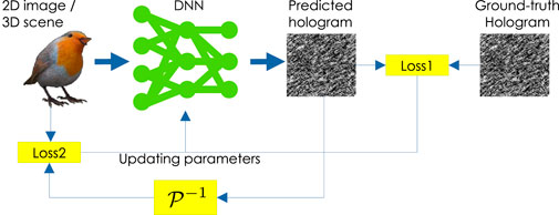
FIGURE 4. Layer-based hologram calculation using deep neural network (Shi et al., 2021).

This DNN was trained using two loss functions. The first loss function, ${\mathcal{L}}_1$, calculates the error between the hologram output from the DNN and the ground-truth hologram. The second loss function, ${\mathcal{L}}_2$, calculates the error between a reproduced image, obtained by an inverse diffraction calculation $({\mathcal{P}}^{-1})$ with the propagation distance z from the predicted hologram, and its corresponding sectional image at z. Here, the hologram output from the DNN is in complex amplitude at an intermediate position between the 3D scene and final hologram. The study Shi et al. (2021) explained the reason for using intermediate holograms as follows:

The convolutional layers of DNN use a 3 × 3 filter. If a 3D scene and hologram are far apart, it is impossible to represent the spread light waves without connecting many convolution layers, making the DNN very large. The DNN outputs a complex hologram at an intermediate position to alleviate the above problem. In the middle position, the light wave does not spread; thus, reducing the number of convolution layers.

Additionally, if the 3D scene and intermediate hologram are sufficiently close, these images will be similar, facilitating the DNN training. The intermediate hologram is propagated to the final hologram plane using the angular spectrum method and converted to an anti-aliased double phase hologram (Hsueh and Sawchuk, 1978; Shi et al., 2021). By displaying the anti-aliased double phase hologram on a phase-only SLM, speckle-free, natural, and high-resolution 3D images can be observed at video rates.

The study trained the DNN using their RGBD image dataset called MIT-CGH-4K. This dataset consists of 4,000 sets of RGBD images and intermediate holograms. It allows DNNs to work well with RGBD images rendered by computer graphics and real RGBD images captured by RGBD cameras. In many DNN-based color 3D reproductions, including this study, the time-division method (Shimobaba and Ito, 2003; Oikawa et al., 2011) is employed. The time-division method enables color reproduction by displaying the holograms of the three primary colors synchronously with the RGB illumination light. However, it requires an SLM capable of high-speed switching.

The trained DNN can generate 1,920, ×, 1,080 pixel holograms at a rate of 60 Hz using a graphics processing unit. It can also generate holograms interactively at 1.1 Hz on a mobile device (iPhone 11 Pro) and at 2.0 Hz on an edge device with Google tensor processing unit (TPU). For the TPU a float 32 precision DNN was compressed into an Int8 precision DNN using quantization, which is one of the model compression methods for DNNs.

2.4 Camera-in-the-Loop Holography

The quality of reproduced images of holographic displays will be degraded because of the following factors: misalignment of optical components (beam splitters and lenses), SLM cover glass, aberrations of optical components, uneven light distribution of a light source on the SLM, and quantized and non-linear light modulation of SLM, as shown in the graph of Figure 5.

FIGURE 5

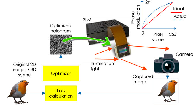
FIGURE 5. Camera-in-the-loop holography.

The GS algorithm, Wirtinger holography, and stochastic gradient methods (Chakravarthula et al., 2019) determine a hologram that yields the desired reproduced image using $\underset{\varphi }{minimize}\mathcal{L}({\mathcal{P}}_{ideal}(\varphi ),a_o)$. Here ϕ, a_o, and $\mathcal{L}$ represent a hologram, target image, and loss function (defined as the error between the target and reproduced images). Successful optimization with this method will be achieved when the actual optical system and ideal light wave propagation model ${\mathcal{P}}_{ideal}$ are consistent.

Although some studies have been conducted to manually correct aberrations to get closer to the ideal propagation model ${\mathcal{P}}_{ideal}$, the camera-in-the-loop holography (Peng et al., 2020) has been proposed to automatically correct these image quality degrading factors. Figure 5 shows the outline of the camera-in-the-loop holography. The camera-in-the-loop holography differs from the GS algorithms, Wirtinger holography, and gradient descent methods because it uses actual reproduced images in the optimization loop.

In the camera-in-the-loop holography, a gradient descent method was used to find an ideal hologram as $\varphi \leftarrow \varphi -\alpha \partial \mathcal{L}/\partial \varphi$, where α is the learning rate, $\mathcal{L}$ is the loss function used to calculate the error between an actual reproduced image captured by a camera and target image, and $\frac{\partial \mathcal{L}}{\partial \varphi }=\frac{\partial \mathcal{L}}{\partial \mathcal{P}}\frac{\partial \mathcal{P}}{\partial \varphi }$, where $\mathcal{P}$ represents the actual optical system, including unknown aberrations. However, the gradient $\frac{\partial \mathcal{P}}{\partial \varphi }$ cannot be calculated due to the unknown parameter. The camera-in-the-loop holography approximates the unknown gradient as follows

$\frac{\partial \mathcal{L}}{\partial \varphi }=\frac{\partial \mathcal{L}}{\partial \mathcal{P}}\frac{\partial \mathcal{P}}{\partial \varphi }\approx \frac{\partial \mathcal{L}}{\partial \mathcal{P}}\frac{\partial {\mathcal{P}}^{\prime }}{\partial \varphi },(6)$

where ${\mathcal{P}}^{\prime }$ is a known propagation model. For example, if ${\mathcal{P}}^{\prime }$ is a free-space propagation between the SLM and reproduced image, it can simply use a diffraction calculation as ${\mathcal{P}}^{\prime }={\mathcal{P}}_{ideal}$. The gradient $\frac{\partial \mathcal{L}}{\partial \mathcal{P}}$ can be calculated using reproduced images captured by a camera.

The following research is an extension of the camera-in-the-loop holography: high-quality holographic display using partially coherent light (LED light source) (Peng et al., 2021), holographic display using Michelson setup to eliminate undiffracted light of SLM (Choi et al., 2021), optimizing binary phase holograms (Kadis et al., 2021), holographic display that suppresses high-order diffracted light using only computational processing without any physical filters (Gopakumar et al., 2021), and further improvement of image quality by using a Gaussian filter to remove noise that is difficult to optimize (Chen et al., 2022).

The above camera-in-the-loop holography needs to be re-optimized for each target image, which can take several minutes. To solve this problem, HoloNet, a combination of camera-in-the-loop holography and DNN, was proposed (Peng et al., 2020). Figure 6 shows a schematic of HoloNet. HoloNet consists of two DNNs and a physically-based calculation (diffraction calculation). The camera is required for the training stage of the DNN; however, it is not required for the inference stage. DNN1 outputs the optimal phase distribution of the target image. The phase distribution and target image are combined to form a complex amplitude. Then, a Zernike-compensated diffraction calculation is performed by considering the aberrations of the optical system. DNN2 transforms the complex amplitude obtained by the diffraction calculation into a phase-only hologram suitable for SLM. HoloNet can generate full-color holograms with 2K resolution at 40 frames per second.

FIGURE 6

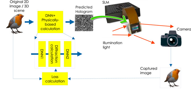
FIGURE 6. HoloNet: a combination of camera-in-the-loop holography and deep neural network (Peng et al., 2020).

Chakravarthula et al. (2020) proposed an aberration approximator. The aberration approximator uses a U-Net-based DNN. The DNN infers the aberrations of an optical system to obtain holograms that are corrected for the aberrations. The conditional GAN (Isola et al., 2017) was used to train the DNN, and the training datasets were numerical reproduced images of holograms generated assuming an ideal optical system and reproduced images from the actual optical system captured by a camera.

Kavaklı et al. (2022) pointed out that the algorithms of Wu et al. (2021) and Peng et al. (2020) are complex processing. The study Kavaklı et al. (2022) obtained an optimized point spread function for diffraction calculation from the error between numerically reproduced images from holograms calculated from the ideal diffraction calculation and the actual reproduced images captured by a camera. It is worth noting that the optimized point spread function has an asymmetric distribution different from the point spread function in the ideal case. Additionally, the optimized point spread function reflects the aberrations of the optical system. We can obtain holograms that give an ideal reproduction image by calculating holograms with the optimized point spread function.

2.5 Other Applications Using Deep Neural Network

2.5.1 Image Quality Enhancement

A reproduced image of a hologram calculated using random phase will have speckle noise. Park and Park (2020) proposed a method for removing speckle noise from random phase holograms. In this method, the reproduced image (light-field data) is first numerically computed from a random phase hologram. Since the reproduced light-field data also contains speckle noise, this method employs a denoising convolutional neural network (Zhang et al., 2017a) to remove this noise. Furthermore, a speckle-free reproduction image can be observed by recalculating the hologram from the speckle-free light-field data.

Ishii et al. (2022) proposed the image quality enhancement of zoomable holographic projections using DNNs. To obtain a reproduced image larger than the hologram size, it is necessary to use a random phase; however, this gives rise to speckle noise. The random phase-free method (Shimobaba and Ito, 2015), which applies virtual spherical waves to the original image and calculates the hologram using a scaled diffraction calculation (Shimobaba et al., 2013), can avoid this problem. However, it does not apply well to phase-only holograms. A DNN of (Ishii et al., 2022) converts a phase-only hologram computed using the random phase-free method in an optimized phase-only hologram. Two layers for computing the forward and inverse scaled diffraction (Shimobaba et al., 2013) are introduced before and after DNN. Then, the DNN is trained using unsupervised learning, as discussed in Section 2.2. In the inference, the two layers are removed, and a phase-only hologram is computed using the random phase-free method and a scaled diffraction calculation is input to the DNN to optimize a zoomable phase-only hologram.

2.5.2 Hologram Compression

The amount of data in holograms is a major problem. Data compression is essential for real-time hologram transmission and wide-viewing-angle holographic displays, which require holograms with large spatial bandwidth products. Existing compression techniques [e.g., JPEG, JPEG 2000, and high-efficiency video coding (HEVC)] and distinctive compression techniques have been proposed (Blinder et al., 2014; Birnbaum et al., 2019; Stepien et al., 2020), which aim to take the distinctive signal properties of digital holograms into account. Compression of hologram data is not easy because holograms have different statistical properties from general natural images, so standard image and video codecs will achieve sub-optimal performance. Several DNN-based hologram data compression algorithms have been proposed to address this matter.

When JPEG or other compression algorithms targeted to natural image date are used for hologram compression, essential high-frequency components are lost, and block artefacts will perturb the hologram viewing. In Jiao et al. (2018), a simple DNN with three convolution layers was used to restore the JPEG-compressed hologram close to the original one. The DNN learns the relationship between the JPEG-degraded hologram and the original hologram using end-to-end learning. Although it was tested on JPEG, it can easily be applied to other compression methods, making it highly versatile.

In Shimobaba et al. (2019a) and Shimobaba et al. (2021a), holograms were compressed through binarization using the error diffusion method (Floyd, 1976). The U-Net-based DNN restored binary holograms to the original grayscale. If the input hologram is 8 bits, the data compression ratio is 1/8. DNN can obtain better reproduction images than JPEG, JPEG2000, and HEVC at the same bit rate.

2.5.3 Hiding of Information in Holograms

Steganography is a technique used to hide secret images in a host image (also called cover image). The hidden images must not be known to others. A closely related technique is watermarking: it embeds copyright information (e.g., a copyright image) in the host image. The copyright information can be known by others, but it must be impossible to remove. These techniques are collectively referred to as information hiding. Many holographic information hiding techniques have been proposed (Jiao et al., 2019). For example, the hologram of a host image can be superimposed on that of a hidden image to embed hidden information (Kishk and Javidi, 2003). The hidden information should be encrypted with double random phase encryption (Refregier and Javidi, 1995) to prevent it from being read. An important difference with digital information hiding is that holographic information hiding allows for optical encryption and decryption of the hidden image, and handling 3D host and hidden information.

The combination of holographic information hiding and DNN can improve the resistance to attacks and the quality of decoded images. In Wang et al. (2021), the holograms of host and hidden images were superimposed on a single hologram using a complementary mask image. Each hologram was converted into a phase-only hologram by patterned-phase-only holograms (Tsang et al., 2017). The hologram of the hidden image is encrypted with double random phase encryption (Refregier and Javidi, 1995). When the final hologram is reconstructed, we can observe only the host image. Since the mask image is the key, we can observe the hidden image when the mask image is multiplied with the hologram, but the image quality is considerably degraded. This degradation is recovered using a DNN; DenseNet (Huang et al., 2017) was used as the DNN. It is trained by end-to-end learning using the dataset of degraded and ground-truth hidden images.

In Shimobaba et al. (2021b), a final hologram u recorded a hologram u_h of a host image and a hologram u_e of a hidden image was calculated as $u={\mathcal{P}}_{z_1}\{u_h\}+\alpha {\mathcal{P}}_{z2}\{u_e\}$. Here, ${\mathcal{P}}_z$ is the diffraction calculation of the propagation distance z; z₁ and z₂ are the distance between the hologram and each image; α is the embedding strength of the hidden hologram. We can make the reproduced hidden image less noticeable by making α sufficiently small. Here, it was set to 4% of the amplitude of the host hologram. It is not easy to identify the reproduced hidden image at this value. Therefore, if we want to identify it, DNN recovers the hidden image. The DNN was trained using reproduced hidden and ground-truth hidden images. U-Net and ResNet were used as the network structure. Both networks could recover the hidden images.

3 Digital Holography Using Deep Learning

In digital holography (Goodman and Lawrence, 1967; Kim, 2010; Liu et al., 2018; Tahara et al., 2018) image sensors are used to capture holograms of real macroscale objects and cells. It is possible to obtain a reproduced image from the hologram using diffraction calculation. Digital holography has been the subject of much research in 3D sensing and microscopy. Figure 7 shows the process of digital holography. We calculate a diffraction calculation from a hologram captured by an image sensor to obtain a reproduction image in a computer. If the reconstructed position of the target object needs to be known accurately, autofocusing is required to find the focus position by repeating diffraction calculations. Autofocusing looks for a position where the reconstructed image is sharp. Aberrations are superimposed due to optical components and alignment errors. Meanwhile, it is necessary to correct this aberration. Since digital holography can obtain complex amplitudes, simultaneous measurement of amplitude and phase is possible. The phase can be obtained by calculating the argument of a complex value using the arctangent function, but its value range is wrapped into $\left[-\pi ,+\pi \right)$. Therefore, phase unwrapping is required to reproduce the thickness of an object from its phase.

FIGURE 7

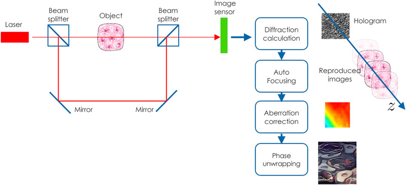
FIGURE 7. Process flow of digital holography.

However, the above processes are time-consuming computations. In this section, we introduce digital holography using DNNs. We can speed up some (or all) of the time-consuming processing using DNNs. Furthermore, DNNs have successfully obtained reproduced images with better image quality than conventional methods. For a more comprehensive and detailed description of digital holography using DNNs, see review papers Rivenson et al. (2019), Javidi et al. (2021), and Zeng et al. (2021).

3.1 Depth Estimation

A general method for estimating the focus position is to obtain the most focused position by calculating reproduced images at different depths from the hologram. The focus position is determined using metrics, such as entropy, variance, and Tamura coefficient (Zhang et al., 2017b). This process requires an iterative diffraction calculation, which is computationally time-consuming. An early investigation of autofocusing using DNNs was to estimate the depth position of a target object from a hologram. The depth prediction can be divided into two categories: classification and regression problems.

Pitkäaho et al. (2019) proposed the depth position prediction as a classification problem. They showed that DNNs for classification commonly used in the MNIST classification problem could classify the range of 260–272 mm, where the target object is located, into five depths at 3 mm intervals.

DNNs for estimating the depth location as a regression problem (Ren et al., 2018; Shimobaba et al., 2018) infer a depth value z directly from a hologram image (or its spectrum) H. This network is similar to that of the classification problem but with only one neuron in the output layer. The training is performed using end-to-end learning as $\underset{\mathrm{\Theta }}{minimize}\mathcal{L}(\mathcal{N}(H;\mathrm{\Theta }),z)$, where z is the ground-truth depth value. The MSE and other metrics are usually used as loss functions. We can obtain a focused reproduced image through a diffraction calculation using the estimated depth distance from a hologram.

3.2 Phase Unwrapping

Phase unwrapping in physically-based calculation (Ghiglia and Pritt, 1998) connects wrapped phases to recover the thickness (or optical path length) of a target object. Phase unwrapping algorithms have global, region, path-following, and quality-guided algorithms. Additionally, a method that applies the transport intensity equation has been proposed (Martinez-Carranza et al., 2017). These methods are computationally time-consuming.

Many methods have been proposed to perform phase unwrapping by training DNNs with end-to-end learning using a dataset of wrapped phase and their unwrapping images (Wang et al., 2019a; Qin et al., 2020). Once trained, DNNs can rapidly generate unwrapped phase images. Phase unwrapping using Pix2Pix (Isola et al., 2017), a type of generative adversarial network (GAN) (Goodfellow et al., 2014), has been proposed (Park et al., 2021). Pix2Pix can be thought of as a supervised GAN. This study prepared a dataset of wrapped phase and their unwrapped phase images generated using the quality-guided algorithm (Herráez et al., 2002). The U-Net-based generator employs this dataset to generate a realistic unwrapped phase image from the unwrapped phase image to fool the discriminator. The discriminator is trained to detect whether it concerns a generated or real unwrapped phase image. Such adversarial learning can produce high-quality unwrapped images.

3.3 Direct Reconstruction Using the Deep Neural Network

As a further development, research has been conducted to obtain aberration-eliminated, autofocusing, and phase unwrapping images directly by inputting holograms into DNNs.

3.3.1 Supervised Learning

A reproduced image can be obtained by propagating holograms captured by inline holography back to the object plane. However, since the reproduced image contains a twin image and direct light, it is necessary to remove unwanted lights using physically-based algorithms, e.g., phase recovery algorithms. This requires multiple hologram recordings and computational costs for diffraction calculations.

Rivenson et al. (2018) inputs a reproduced image obtained using an inverse diffraction calculation $({\mathcal{P}}^{-1})$ to the object plane into a DNN $(\mathcal{N})$ to obtain a twin image-free reproduced image. The prepared dataset consists of a hologram H and a ground-truth complex amplitude field $\mathcal{Y}$. Then, they trained the DNN using end-to-end learning as $\underset{\mathrm{\Theta }}{minimize}\mathcal{L}(\mathcal{N}({\mathcal{P}}^{-1}(H);\mathrm{\Theta }),\mathcal{Y})$. They used MSE as the loss function $\mathcal{L}$. The ground-truth complex amplitudes were obtained from eight holograms with different recording positions using the multiheight phase retrieval algorithm (Greenbaum and Ozcan, 2012). This study showed that this DNN could reproduce images comparable to those obtained using the multiheight phase retrieval algorithm without time-consuming phase recovery.

Although the study of Rivenson et al. (2018) required the results of propagation calculations from a hologram to be input to the DNN, eHoloNet (Wang et al., 2018) developed DNN that does not require propagation calculations and directly infers object light from a hologram. They created a dataset consisting of a hologram $\mathcal{H}$ and its ground-truth object light $\mathcal{Y}$. The DNN was trained with the following end-to-end learning: $\underset{\mathrm{\Theta }}{minimize}\mathcal{L}(\mathcal{N}(H;\mathrm{\Theta }),\mathcal{Y})$. MSE was used as the loss function $\mathcal{L}$. They employed phase distributions displayed on SLM for collecting ground-truth object lights instead of real objects.

Y-Net (Wang et al., 2019b) separates the upsampling path of U-Net (Ronneberger et al., 2015) into two parts and outputs the intensity and phase of a reproduced image. The dataset includes captured holograms and their ground-truth intensity and phase images. Y-Net is trained using end-to-end learning. Compared with the case where the output layer of U-Net has two channels, and each channel outputs an intensity image and a phase image, Y-Net has successfully obtained better reproduction images.

Y4-Net (Wang et al., 2020a) extends the Y-Net upsampling paths by four for use in dual-wavelength digital holography (Wagner et al., 2000). Dual-wavelength holography uses two wavelengths, λ₁ and λ₂, to make synthetic wavelength for long wavelength measurements λ₁λ₂/(λ₁ − λ₁) and short wavelength measurements λ₁λ₂/(λ₁ + λ₁). Y4-Net outputs the real and imaginary parts of the reproduced image at each wavelength by inputting holograms captured at λ₁ and λ₂.

The above researches are about digital holographic measurement of microorganisms and cells. However, 3D particle measurement is essential to understand the spatial behavior of tiny particles, such as bubbles, aerosols, and droplets. It is applied to flow path design of flow cytometers, environmental measurement, and 3D behavior measurement of microorganisms. Digital holographic particle measurement can measure one-shot 3D particles; however, it requires time-consuming post-processing using diffraction calculations and particle position detection. 3D particle measurement using holography and DNN has been proposed. The study Shimobaba et al. (2019b) prepared a dataset consisting of holograms and their particle position images, a 2D image showing the 3D position of the particle. The position of a pixel indicates the position of the particle in the plane, and its color indicates the depth position of the particle. U-Net was trained using end-to-end learning with the dataset. The DNN can transform holograms to particle position images. The effectiveness of the method was confirmed by simulation.

The study of Shimobaba et al. (2019b) was conducted using simple end-to-end learning. However, Shao et al. (2020) inputs two more pieces of information (depth map and maximum phase projection, both obtained by preprocessing the hologram) to their U-Net in addition to holograms. Additionally, by developing a loss function, this study successfully obtained 3D particle images with a particle density 300 times higher than that of Shimobaba et al. (2019b).

Chen et al. (2021) incorporated compressive sensing into DNN and trained it using end-to-end learning. The input of the DNN were 3D particle holograms, whereas the output was 3D volume data of the particles. Unlike (Shimobaba et al., 2019b; Shao et al., 2020), Zhang et al. (2022) used the Yolo network (Joseph et al., 2016). When a hologram is an input to the DNN, it outputs a 6D vector containing a boundary box that indicates the location of the particle, its objectiveness confidence, and the depth position of the particle.

3.3.2 Unsupervised Learning

End-to-end learning requires a dataset consisting of a large amount of paired data (captured hologram and object light recovered using physically-based algorithms). Since the interference fringes of holograms vary significantly depending on the holographic recording conditions and target objects, there is no general-purpose hologram dataset. Therefore, it is necessary to create an application-specific datasets, which requires much effort. Unsupervised learning is also used for DNNs for digital holography.

Li et al. (2020) showed that using a deep image prior (Ulyanov et al., 2018), a twin image-free reproduced image can be obtained using only a captured inline hologram without large datasets. Furthermore, an auto-encoder was used for the DNN network structure. The deep image prior (Ulyanov et al., 2018) initializes the DNN with random values and inputs a fixed image to the DNN for training. For example, the deep image prior can be used to denoise an image from noisy input. This technique works due to the fact that DNNs are not good at representing noise. The deep image prior is also useful for super-resolution and in-painting. In Li et al. (2020), DNN was trained using the following unsupervised learning: $\underset{\mathrm{\Theta }}{minimize}\mathcal{L}(\mathcal{P}(\mathcal{N}({\mathcal{P}}^{-1}(H_{\text{fix}});\mathrm{\Theta })),H_{\text{fix}})$, where H_fix is a captured inline hologram, and $\mathcal{N}$ is the DNN with the network parameter Θ. The reproduced image of an inline hologram $({\mathcal{P}}^{-1}(H_{\text{fix}}))$ includes a twin image, which can be considered noise. By inputting the noisy reproduced image into the DNN, the DNN outputs the complex amplitude field of the target object with reduced twin image using the principle of the deep image prior. This study conducted a diffraction calculation $(\mathcal{P})$ of the DNN output to generate a hologram. It learns Θ to minimize the error between computed and captured holograms. Consequently, the study obtained that the quality of a reproduced image is better than using a state-of-the-art compressed sensing (Zhang et al., 2018b).

PhysenNet (Wang et al., 2020b) was also inspired by the deep image prior. PhysenNet can infer the phase image of a phase object by inputting its hologram into a DNN. The network is a U-Net, trained using the following unsupervised learning: $\underset{\mathrm{\Theta }}{minimize}\mathcal{L}(\mathcal{P}(\mathcal{N}(H_{\text{fix}}));\mathrm{\Theta })\left.\right),H_{\text{fix}}\left.\right)$. The phase distribution output from the DNN is computed by diffraction to generate holograms. The DNN is trained to minimize the error between the measured and generated holograms. The minimization formula is slightly different from Li et al. (2020).

3.3.3 Generative Adversarial Network

GANs (Goodfellow et al., 2014), one of the training methods for DNNs, have been widely used in computational holography because of their excellent image transformation capabilities.

Liu et al. (2019a) used the conditional GAN for super-resolution in digital holographic microscopy. Conditional GAN is a method that adds ground-truth information to GAN; it is a supervised learning method. Figure 8 shows a schematic of Liu et al. (2019a). As shown in the figure, $\mathcal{X}$ is the low-resolution hologram; $\mathcal{G}$ is the generating network (using U-Net); $\mathcal{G}(\mathcal{X})$ is the high-resolution hologram output from the generating network; $\mathcal{Z}$ is a ground-truth high-resolution hologram; $\mathcal{D}$ is a discriminating network that can distinguish whether a high-resolution hologram is a generated or a ground-truth hologram. The datasets of low- and high-resolution holograms are taken with on-chip digital holographic microscopy. The high-resolution holograms are captured by changing objective lenses with different numerical apertures. Alternatively, the image sensor can be laterally shifted to capture multiple low-resolution holograms, which are super-resolved using the physically-based algorithm (Greenbaum et al., 2014) to generate high-resolution holograms.

FIGURE 8

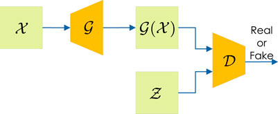
FIGURE 8. Architecture of a conditional generative adversarial network.

Similar to Liu et al. (2019a), Liu et al. (2019b) employed the conditional GAN to generate accurate color images from holograms captured at three wavelengths suitable for point-of-care pathology. Conditional GAN can produce holographic images with high accuracy. However, a dataset must be prepared since it is supervised learning, which requires much effort. To overcome this problem, holographic microscopy using cycle GANs with unsupervised learning has been investigated (Yin et al., 2019; Zhang et al., 2021).

3.4 Interconversion Between Holographic and Other Microscopes

Many microscopes, such as bright-field, polarized light, and digital holographic microscopes, have been developed, each with its strengths and weaknesses. Interconversion between the reproduced image of a holographic microscope and that of another microscope has been investigated using deep learning. It has become possible to overcome each other’s shortcomings. In many cases, GANs, which are excellent at transforming images, are used to train DNNs.

Bright-field microscopy allows simple observation of specimens using a white light source; however, transparent objects must be stained. Additionally, only 2D amplitude information of a target object can be obtained due to the shallow depth of focus. Wu et al. (2019) showed that digital holographic reproduced images could be converted to bright-field images using GAN. In contrast, Go et al. (2020) converted an image taken by bright-field microscopy into a hologram. They showed that it is possible to recover the 3D positional information of particles from this hologram. Additionally, they developed a system that can capture bright-field and holographic images simultaneously to create a dataset. The GAN generator produces holograms from bright-field images, and the discriminator is trained to determine whether it is a generated or captured hologram.

Liu et al. (2020) converted the reproduced image of digital holographic microscopy into a polarized image of polarized light microscopy. Polarized light microscopy has problems, such as a narrow field of view and the need to capture several images with different polarization directions. The study Liu et al. (2020) showed that a DNN trained by a GAN could infer a polarization image from a single hologram. The dataset consists of data pairs of holograms taken using a holographic microscope and polarized light images taken with single-shot computational polarized light microscopy (Bai et al., 2020) of the same object.

3.5 Holographic Classification

Holographic digital microscopy can observe the phase of transparent objects, such as cells, allowing for label-free observation of cells. By using this feature, a rapid and label-free screening of anthrax using DNN and holographic microscopy has been proposed (Jo et al., 2017). The DNN consists of convolutional layers, MaxPoolings, and classifiers using fully-connected layers.

O’Connor et al. (2020) classified holographic time-series data. They employed a low-cost and compact shearing digital holographic microscopy (Javidi et al., 2018) made with a 3D printer to capture and classify holographic time-series data of blood cells in animals, and healthy individuals, and those with sickle cell disease in humans.

Figure 9 shows a schematic of O’Connor et al. (2020). In the second step of the off-axis phase reconstruction, only the object light component is Fourier filtered, as in a conventional off-axis hologram, to obtain the phase image in the object plane using a diffraction calculation (Takeda et al., 1982; Cuche et al., 2000). The feature extractor extracts features from the phase image. The manually extracted and automatically extracted features from DNNs, which are transfer-learned from DenseNet (Huang et al., 2017), are input to a long short-term memory network (LSTM) to classify the cells. LSTM is a recurrent neural network (RNN). RNNs have a gradient vanishing problem as the time-series data become longer; however, LSTMs can solve this problem. The study O’Connor et al. (2020) showed that LSTM significantly improved the classification rate of the cells compared to traditional machine learning methods, such as the random forest and support vector machine. The classification of spatiotemporal COVID-19 infected and healthy erythrocytes was reported (O’Connor et al., 2021) using this technique.

FIGURE 9

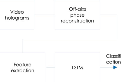
FIGURE 9. Classification of time-series hologram of cells.

4 Faster Deep Neural Networks

Deep learning, as introduced above, entails a neural network running on semiconductors. The switching speed of transistors governs its speed, and its power consumption is high. To solve this problem, an optical neural network has been proposed (Goodman and Goodman, 2005; Genty et al., 2021).

Research on optical computers has a long history. For example, pattern recognition by optical computing was reported in 1964 (Vander LUGH, 1964). This research used optical correlation to perform simple recognition. Optical computers use a passive hologram used as a modulator of light. Therefore, it requires little power and can perform the recognition process at exactly the speed of light. Research has been recently conducted on optical deep learning (Genty et al., 2021). In this study, we introduce one of them, the diffractive DNN (D²NN), which is closely related to holography (Lin et al., 2018).

Figure 10 shows the D²NN and semiconductor-based DNN. A D²NN modulates the input light modulated by some information with multiple diffractive layers (holograms). It learns the amplitude and phase of the diffractive layers to strengthen the light intensity of the desired detector. For example, in the case of classification, the input light of the classification target is modulated in each diffractive layer, and the diffractive layer is learned to strengthen the light intensity of the detector corresponding to the target. Existing deep-learning frameworks, such as Keras, Tensorflow, or PyTorch, can be used to train the diffractive layers.

FIGURE 10

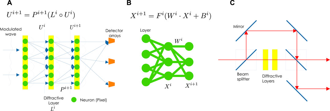
FIGURE 10. Diffractive deep neural network: (A) D²NN, (B) semiconductor-based DNN (B), and (C) D²NN incorporating the ideas of ResNet.

In Figure 10A, a light wave Uⁱ is diffracted by ith diffractive layer. The propagated light wave Uⁱ⁺¹ before the next diffractive layer is expressed as follows:

$U^{i+1}={\mathcal{P}}^{i+1}\left(L^i◦U^i\right),(7)$

where ${\mathcal{P}}^{i+1}$ is the diffraction between the layers of i and i + 1, and ◦ is the Hadamard product. For ${\mathcal{P}}^i$, general diffraction calculations, such as the angular spectrum method, can be used. The forward calculation of D²NN is completed by iterating Eq. 7 as many times as the number of diffractive layers.

Since the calculation of Eq. 7 consists of the entirely differentiable operations, each diffractive layer can be optimized by automatic differentiation from the forward calculation. The D²NN is trained on a computer, and the trained diffractive layers are recorded on an optical modulator (photopolymer or SLM). These optical modulators correspond to the layers of the semiconductor-based DNN. A D²NN can be constructed by arranging these layers in equal intervals. The classification rate can be further improved (Watanabe et al., 2021) by arranging the diffractive layers in a non-equally spaced manner. The spacing of diffractive layers is a hyperparameter, which is not easy to tune manually. Watanabe et al. (2021) employed a Bayesian optimization technique, the tree-structured Parzen estimator (James et al., 2011), for hyperparameter tuning.

Figure 10B shows a semiconductor-based DNN. The output Xⁱ⁺¹ of the input Xⁱ at the ith layer of this DNN can be expressed by

$X^{i+1}=F^i\left(W^i\cdot X^i+B^i\right),(8)$

where Wⁱ is the weight parameters, B_i is the bias (not shown in the figure), ⋅ is the matrix product, and Fⁱ is the activation function. Semiconductor-based DNNs can represent arbitrary functions because Eq. 8 contains nonlinear activation functions. However, Eq. 7 of D²NN has no activation function; therefore, it can only handle linear problems. Still, there are many applications where D²NNs work effectively for linear problems.

The study Lin et al. (2018) investigated the MNIST classification accuracy using D²NN. When a five-layer D²NN was validated through simulation, it achieved a 91.75% classification rate. Meanwhile, the classification rate improved to 93.39% for a seven-layer. The state-of-the-art classification rate for electrical DNNs was 99.77%. When the layers were 3D printed and optically tested, a classification rate of 88% was achieved despite the manufacturing and alignment errors of the layers.

D²NNs are usually constructed with relatively shallow layers. Dou et al. (2020) applied the idea of ResNet (He et al., 2016) to D²NN and reduced the gradient vanishing problem in deep diffractive layers. ResNet reduced gradient vanishing by introducing shortcuts, whereas Res-D²NN (Dou et al., 2020) introduces optical shortcut connections, as shown in Figure 10C. When a 20-layer D²NN and Res-D²NN were run through the MNIST classification problem, the identification rates were 96.0% and 98.4%, respectively, with the Res-D²NN showing superior performance.

Sakib Rahman and Ozcan (2021) showed through simulations that a twin image-free holographic reproduced image could be obtained using a D²NN. When holograms captured by inline digital holography are reproduced, blurry conjugate light is superimposed on the object light. Phase recovery algorithms, compressive sensing, and deep learning are used to remove this conjugate light, all of which operate on semiconductors. The study Sakib Rahman and Ozcan (2021) trained a D²NN to input light from a hologram into the D²NN and pass it through several diffractive layers to obtain a twin image-free reproduced image. The loss function $\mathcal{L}$ is defined as follows:

$\mathcal{L}=\Vert I-\mathcal{Y}{\Vert }_2+{\alpha }_1\Vert \mathcal{F}\left(I\right)-\mathcal{F}\left(\mathcal{Y}\right){\Vert }_2+{\alpha }_2\left(1-P_I/P_{illum}\right),(9)$

where ‖⋅‖₂ denotes the ℓ2 norm, and the first term is the error between the inferred image I of D²NN and the ground-truth image $\mathcal{Y}$; the second term is the spectral error; the third term is the diffraction efficiency defined as the ratio of the power P_I of the reproduced image to the total power P_illum of the illumination light. The third term subtracts the diffraction efficiency from 1 so that the loss function becomes smaller as the diffraction efficiency increases. α₁ and α₂ are hyperparameters. The amount of modulation of the diffractive layers is determined by minimizing this loss function.

5 Our Personal View and Discussion

In previous sections, we introduced computational holography, including computer-generated holograms, holographic displays, digital holography, and D²NN, using deep learning. Several studies have shown that deep learning outperforms existing physically-based calculations. In this section, we briefly discuss our personal view on deep learning.

Algorithms for computer-generated hologram in holographic display include point-cloud, polygon, layer, and light-field methods. Several physically-based algorithms have been proposed for layer methods (Okada et al., 2013; Chen et al., 2014; Chen and Chu, 2015; Zhao et al., 2015). The DNN-based method (Shi et al., 2021) proposed by Shi et al. (2021) has been a near-perfect layer method in computational speed and image quality. Physically-based layer methods are inherently computationally expensive due to the iterative use of diffraction calculations. The DNN in Shi et al. (2021) skips this computational process and can map input RGBD images directly to holograms. This study showed that DNN could generate holograms two orders of magnitude faster than sophisticated physically-based layer methods.

Holograms generated using the layer method are suitable for holographic near-eye display because a good 3D image can be observed from the front of holograms (Maimone et al., 2017). These holograms have a small number of hologram pixels. Additionally, since the holograms do not need to have a wide viewing angle, they have only low-frequency interference fringes, indicating low spatial bandwidth product (Blinder et al., 2019). These features are suitable for DNNs, which is why current hologram generation using DNNs is mainly for layer holograms. Holograms with a large spatial bandwidth product have a wide viewing angle, allowing a large 3D image to be observed by many people. However, this would require large-scale holograms. Such holograms require a pixel pitch of about a wavelength and billions to tens of billions of pixels (Matsushima and Sonobe, 2018; Matsushima, 2020). Holograms are formed from high-frequency interference fringes, and hologram patterns appear noisy at first glance. Current DNNs have difficulty handling such large-scale holograms due to memory issues and computational complexity. Additionally, deep image prior (Ulyanov et al., 2018) points out that current DNNs based on convolutions are not good at generating noisy patterns. Therefore, hologram generation with large spatial bandwidth products using DNNs is a big challenge.

Since DNNs were developed from image identification, RGBD images used in the layer method are suitable for DNNs. However, it is not easy for DNN to handle coordinate data formats used in the point cloud and polygon methods. So far, few studies exist on how to handle the point cloud method (Kang et al., 2021) using DNN. The authors look forward to further progress in these studies.

Deep learning is a general-purpose optimization framework that can be used in any application involving signals. However, it is difficult to answer whether it can outperform existing methods in all applications and use cases. Using optical cryptography and single-pixel imaging as examples, Jiao et al. (2020) compared a well-known linear regression method (GeorgeSeber and AlanLee, 2012) with deep learning. They concluded that the linear regression method is superior in both applications. DNNs require a lot of tuning: tuning the network structure and hyperparameters, selecting appropriate loss functions and optimizers, and preparing a large dataset. If we tune them properly, which is not necessary in existing physically-based methods, we may obtain excellent results. However, it requires much effort. Ultimately, deep learning is a sophisticated fitting technique, so analytical models matching the ground truth physics may be favorable whenever knowable and efficiently computable. Thus, it is essential to choose appropriate physically-based methods and deep learning in the future.

Deep learning requires the preparation of a large number of datasets, which generally require much effort. Computer-generated holograms using DNNs also require the preparation of datasets; however, they can be generated on a computer. Therefore, there is no need to take holograms with an actual optical system, except for systems such as the camera-in-the-loop holography. Digital holography is more problematic, as it requires a great deal of effort to acquire information about target objects and their holograms. Unsupervised learning, as discussed in Section 3.3, is ideal. However, unlike DNNs trained in supervised and unsupervised manners, phase recovery algorithms and compressed sensing can recover target object lights using only few known information about the target objects. Thus, they do not require a dataset. For supervised learning, DNNs should be trained by generating data pairs of holograms and their object lights using phase recovery algorithms and compressed sensing, as stated in Rivenson et al. (2018).

The generalization performance of DNNs is also essential. For example, in the case of digital holography, there is no guarantee that a DNN trained on a dataset with a particular object and optical system will be able to accurately recover object lights from holograms captured in other situations. Therefore, to improve the generalization performance of DNNs, we can use datasets that include various types of data, and techniques such as domain adaptation (Tzeng et al., 2017), which has been the subject of much research in recent years.

Furthermore, DNNs have outperformed physically-based calculations in many applications of computational holography. So, will there still be a need for physically-based calculations in the future? The answer is yes, because DNNs require large datasets which need to be generated using sophisticated physically-based calculations. Additionally, the validity of the results generated using DNNs should be benchmarked with the results obtained using physically-based calculation. Meanwhile, several attempts have been made on introducing layers of physically-based calculations in DNNs (Rivenson et al., 2018; Wang et al., 2020b; Hossein Eybposh et al., 2020; Li et al., 2020; Chen et al., 2021; Horisaki et al., 2021; Shi et al., 2021; Wu et al., 2021; Ishii et al., 2022; Kavaklı et al., 2022). Therefore, it will be necessary to continue research on physically-based calculations in terms of speed and image quality to speed up these layers.

6 Conclusion

In this review, we comprehensively introduced computational holography, including computer-generated holography, holographic display, digital holography using deep learning, and D²NNs using holographic technology. Computational holography using deep learning has outperformed conventional physically-based calculations in several applications. Additionally, we briefly discussed our personal view on the relationship between DNNs and physically-based calculations. Based on these discussions, we believe that we need to continue research on deep learning and physically-based calculations. The combination of deep learning and physically-based calculations will further lead to a groundbreaking computational holography research.

Author Contributions

TS, DB, and TB wrote the manuscript. TS, DB, TB, IH, HS, PS, and TI also discussed the techniques introduced in the manuscript and reviewed the manuscript.

Funding

This research was funded by the joint JSPS–FWO scientific cooperation program (VS07820N), FWO Junior postdoctoral fellowship (12ZQ220N), and the Japan Society for the Promotion of Science (19H04132 and JPJSBP120202302).

Conflict of Interest

The authors declare that the research was conducted in the absence of any commercial or financial relationships that could be construed as a potential conflict of interest.

Publisher’s Note

All claims expressed in this article are solely those of the authors and do not necessarily represent those of their affiliated organizations, or those of the publisher, the editors and the reviewers. Any product that may be evaluated in this article, or claim that may be made by its manufacturer, is not guaranteed or endorsed by the publisher.

References

Ahrenberg, L., Benzie, P., Magnor, M., and Watson, J. (2008). Computer Generated Holograms from Three Dimensional Meshes Using an Analytic Light Transport Model. Appl. Opt. 47 (10), 1567–1574. doi:10.1364/ao.47.001567

PubMed Abstract | CrossRef Full Text | Google Scholar

Bai, B., Wang, H., Liu, T., Rivenson, Y., FitzGerald, J., and Ozcan, A. (2020). Pathological crystal Imaging with Single-Shot Computational Polarized Light Microscopy. J. Biophotonics 13 (1), e201960036. doi:10.1002/jbio.201960036

PubMed Abstract | CrossRef Full Text | Google Scholar

Birnbaum, T., Ahar, A., Blinder, D., Schretter, C., Kozacki, T., and Schelkens, P. (2019). Wave Atoms for Digital Hologram Compression. Appl. Opt. 58 (22), 6193–6203. doi:10.1364/AO.58.006193

PubMed Abstract | CrossRef Full Text | Google Scholar

Blinder, D., Ahar, A., Bettens, S., Birnbaum, T., Symeonidou, A., Ottevaere, H., et al. (2019). Signal Processing Challenges for Digital Holographic Video Display Systems. Signal. Processing: Image Commun. 70, 114–130. doi:10.1016/j.image.2018.09.014

CrossRef Full Text | Google Scholar

Blinder, D., Bruylants, T., Ottevaere, H., Munteanu, A., and Schelkens, P. (2014). Jpeg 2000-based Compression of Fringe Patterns for Digital Holographic Microscopy. Opt. Eng. 53 (12), 123102. doi:10.1117/1.oe.53.12.123102

CrossRef Full Text | Google Scholar

Blinder, D., and Schelkens, P. (2020). Phase Added Sub-stereograms for Accelerating Computer Generated Holography. Opt. Express 28 (11), 16924–16934. doi:10.1364/oe.388881

PubMed Abstract | CrossRef Full Text | Google Scholar

Buckley, E. (2011). Holographic Laser Projection. J. Display Technol. 7 (3), 135–140. doi:10.1109/jdt.2010.2048302

CrossRef Full Text | Google Scholar

Chakravarthula, P., Peng, Y., Kollin, J., Fuchs, H., and Heide, F. (2019). Wirtinger Holography for Near-Eye Displays. ACM Trans. Graph. 38 (6), 1–13. doi:10.1145/3355089.3356539

CrossRef Full Text | Google Scholar

Chakravarthula, P., Tseng, E., Srivastava, T., Fuchs, H., and Heide, F. (2020). Learned Hardware-In-The-Loop Phase Retrieval for Holographic Near-Eye Displays. ACM Trans. Graph. 39 (6), 1–18. doi:10.1145/3414685.3417846

CrossRef Full Text | Google Scholar

Chang, C., Bang, K., Wetzstein, G., Lee, B., and Gao, L. (2020). Toward the Next-Generation Vr/ar Optics: a Review of Holographic Near-Eye Displays from a Human-Centric Perspective. Optica 7 (11), 1563–1578. doi:10.1364/optica.406004

PubMed Abstract | CrossRef Full Text | Google Scholar

Chen, C., Kim, D., Yoo, D., Lee, B., and Lee, B. (2022). Off-axis Camera-In-The-Loop Optimization with Noise Reduction Strategy for High. Opt. Lett. 44, 790–793. doi:10.1364/OL.447871

CrossRef Full Text | Google Scholar

Chen, J.-S., and Chu, D. P. (2015). Improved Layer-Based Method for Rapid Hologram Generation and Real-Time Interactive Holographic Display Applications. Opt. Express 23 (14), 18143–18155. doi:10.1364/oe.23.018143

PubMed Abstract | CrossRef Full Text | Google Scholar

Chen, J.-S., Chu, D., and Smithwick, Q. (2014). Rapid Hologram Generation Utilizing Layer-Based Approach and Graphic Rendering for Realistic Three-Dimensional Image Reconstruction by Angular Tiling. J. Electron. Imaging 23 (2), 023016. doi:10.1117/1.jei.23.2.023016

CrossRef Full Text | Google Scholar

Chen, N., Wang, C., and Heidrich, W. (2021). Holographic 3d Particle Imaging with Model-Based Deep Network. IEEE Trans. Comput. Imaging 7, 288–296. doi:10.1109/tci.2021.3063870

CrossRef Full Text | Google Scholar

Choi, S., Kim, J., Peng, Y., and Wetzstein, G. (2021). Optimizing Image Quality for Holographic Near-Eye Displays with Michelson Holography. Optica 8 (2), 143–146. doi:10.1364/optica.410622

CrossRef Full Text | Google Scholar

Cuche, E., Marquet, P., and Depeursinge, C. (2000). Spatial Filtering for Zero-Order and Twin-Image Elimination in Digital off-axis Holography. Appl. Opt. 39 (23), 4070–4075. doi:10.1364/ao.39.004070

PubMed Abstract | CrossRef Full Text | Google Scholar

Dou, H., Deng, Y., Yan, T., Wu, H., Lin, X., and Dai, Q. (2020). Residual D2NN: Training Diffractive Deep Neural Networks via Learnable Light Shortcuts. Opt. Lett. 45 (10), 2688–2691. doi:10.1364/ol.389696

PubMed Abstract | CrossRef Full Text | Google Scholar

FienupFienup, J. R. (1982). Phase Retrieval Algorithms: a Comparison. Appl. Opt. 21 (15), 2758–2769. doi:10.1364/ao.21.002758

PubMed Abstract | CrossRef Full Text | Google Scholar

Floyd, Robert. W. (1976). An Adaptive Algorithm for Spatial gray-scale. Proc. Soc. Inf. Disp. 17, 75–77.

Google Scholar

Gabor, D. (1948). A New Microscopic Principle. nature 161, 777–778. doi:10.1038/161777a0

PubMed Abstract | CrossRef Full Text | Google Scholar

Genty, G., Salmela, L., Dudley, J. M., Brunner, D., Kokhanovskiy, A., Kobtsev, S., et al. (2021). Machine Learning and Applications in Ultrafast Photonics. Nat. Photon. 15 (2), 91–101. doi:10.1038/s41566-020-00716-4

CrossRef Full Text | Google Scholar

GeorgeSeber, A. F., and AlanLee, J. (2012). Linear Regression Analysis. John Wiley & Sons.

Google Scholar

Gerchberg, R. W. (1972). A Practical Algorithm for the Determination of Phase from Image and Diffraction Plane Pictures. Optik 35, 237–246.

Google Scholar

Ghiglia, Dennis. C., and Pritt, Mark. D. (1998). Two-dimensional Phase Unwrapping-Theory, Algorithms, and Software; Chapter 1, 2 and 3. Wiley, 1–99.

Google Scholar

Go, T., Lee, S., You, D., and LeeLee, S. J. (2020). Deep Learning-Based Hologram Generation Using a white Light Source. Sci. Rep. 10 (1), 8977. doi:10.1038/s41598-020-65716-4

PubMed Abstract | CrossRef Full Text | Google Scholar

Goi, H., Komuro, K., and Nomura, T. (2020). Deep-learning-based Binary Hologram. Appl. Opt. 59 (23), 7103–7108. doi:10.1364/ao.393500

PubMed Abstract | CrossRef Full Text | Google Scholar

Goodfellow, I., Pouget-Abadie, J., Mirza, M., Xu, B., Warde-Farley, D., Ozair, S., et al. (2014). Generative Adversarial Nets. Adv. Neural Inf. Process. Syst. 27.

Google Scholar

Goodman, J. W. (2005). in Introduction to Fourier Optics. Editor J. W. Goodman. 3rd ed. (Englewood, CO: Roberts & Co. Publishers), 2005.

Google Scholar

Goodman, J. W., and Lawrence, R. W. (1967). Digital Image Formation from Electronically Detected Holograms. Appl. Phys. Lett. 11 (3), 77–79. doi:10.1063/1.1755043

CrossRef Full Text | Google Scholar

Gopakumar, M., Kim, J., Choi, S., Peng, Y., and Wetzstein, G. (2021). Unfiltered Holography: Optimizing High Diffraction Orders without Optical Filtering for Compact Holographic Displays. Opt. Lett. 46 (23), 5822–5825. doi:10.1364/ol.442851

PubMed Abstract | CrossRef Full Text | Google Scholar

Greenbaum, A., Zhang, Y., Feizi, A., Chung, P. L., Luo, W., Kandukuri, S. R., et al. (2014). Wide-field Computational Imaging of Pathology Slides Using Lens-free On-Chip Microscopy. Sci. Transl Med. 6 (267), 267ra175. doi:10.1126/scitranslmed.3009850

PubMed Abstract | CrossRef Full Text | Google Scholar

Greenbaum, A., and Ozcan, A. (2012). Maskless Imaging of Dense Samples Using Pixel Super-resolution Based Multi-Height Lensfree On-Chip Microscopy. Opt. Express 20 (3), 3129–3143. doi:10.1364/oe.20.003129

PubMed Abstract | CrossRef Full Text | Google Scholar

Hasegawa, S., Hayasaki, Y., and Nishida, N. (2006). Holographic Femtosecond Laser Processing with Multiplexed Phase Fresnel Lenses. Opt. Lett. 31 (11), 1705–1707. doi:10.1364/ol.31.001705

PubMed Abstract | CrossRef Full Text | Google Scholar

He, K., Zhang, X., Ren, S., and Sun, J. (2016). “Deep Residual Learning for Image Recognition,” in Proceedings of the IEEE Conference on Computer Vision and Pattern Recognition, 770–778. doi:10.1109/cvpr.2016.90

CrossRef Full Text | Google Scholar

Herráez, M. A., Burton, D. R., Lalor, M. J., and Gdeisat, M. A. (2002). Fast Two-Dimensional Phase-Unwrapping Algorithm Based on Sorting by Reliability Following a Noncontinuous Path. Appl. Opt. 41 (35), 7437–7444. doi:10.1364/ao.41.007437

PubMed Abstract | CrossRef Full Text | Google Scholar

Hilaire, P. S., Benton, S. A., Lucente, M. E., Jepsen, M. L., Kollin, J., Yoshikawa, H., et al. (1990). Electronic Display System for Computational Holography. Pract. Holography IV Int. Soc. Opt. Photon. 1212, 174–182.

Google Scholar

Hiroshi Yoshikawa, T. Y. H. Y., and Yoshikawa, H. (2011). Computer-generated Image Hologram. 中国光学快报 9 (12), 120006–120009. doi:10.3788/col201109.120006

CrossRef Full Text | Google Scholar

Horisaki, R., Nishizaki, Y., Kitaguchi, K., Saito, M., and Tanida, J. (2021). Three-dimensional Deeply Generated Holography [Invited]. Appl. Opt. 60 (4), A323–A328. doi:10.1364/ao.404151

PubMed Abstract | CrossRef Full Text | Google Scholar

Horisaki, R., Takagi, R., and Tanida, J. (2018). Deep-learning-generated Holography. Appl. Opt. 57 (14), 3859–3863. doi:10.1364/ao.57.003859

PubMed Abstract | CrossRef Full Text | Google Scholar

Hossein Eybposh, M., Caira, N. W., Atisa, M., Chakravarthula, P., and Pégard, N. C. (2020). Deepcgh: 3d Computer-Generated Holography Using Deep Learning. Opt. Express 28 (18), 26636–26650. doi:10.1364/oe.399624

PubMed Abstract | CrossRef Full Text | Google Scholar

Hsueh, C. K., and Sawchuk, A. A. (1978). Computer-generated Double-phase Holograms. Appl. Opt. 17 (24), 3874–3883. doi:10.1364/ao.17.003874

PubMed Abstract | CrossRef Full Text | Google Scholar

Huang, G., Liu, Z., Van Der Maaten, L., and Weinberger, K. Q. (2017). “Densely Connected Convolutional Networks,” in Proceedings of the IEEE Conference on Computer Vision and Pattern Recognition, 4700–4708. doi:10.1109/cvpr.2017.243

CrossRef Full Text | Google Scholar

Ishii, Y., Shimobaba, T., Blinder, D., Tobias, B., Schelkens, P., Kakue, T., et al. (2022). Optimization of Phase-Only Holograms Calculated with Scaled Diffraction Calculation through Deep Neural Networks. Appl. Phys. B 128 (2), 1–11. doi:10.1007/s00340-022-07753-7

CrossRef Full Text | Google Scholar

Isola, P., Zhu, J. Y., Zhou, T., and Efros, A. (2017). “Image-to-image Translation with Conditional Adversarial Networks,” in Proceedings of the IEEE Conference on Computer Vision and Pattern Recognition, 1125–1134. doi:10.1109/cvpr.2017.632

CrossRef Full Text | Google Scholar

James, B., Bardenet, R., Bengio, Y., and Kégl, B. (2011). Algorithms for Hyper-Parameter Optimization. Adv. Neural Inf. Process. Syst. 24.

Google Scholar

Javidi, B., Carnicer, A., Anand, A., Barbastathis, G., Chen, W., Ferraro, P., et al. (2021). Roadmap on Digital Holography [Invited]. Opt. Express 29 (22), 35078–35118. doi:10.1364/oe.435915

PubMed Abstract | CrossRef Full Text | Google Scholar

Javidi, B., Markman, A., Rawat, S., O’Connor, T., Anand, A., and Andemariam, B. (2018). Sickle Cell Disease Diagnosis Based on Spatio-Temporal Cell Dynamics Analysis Using 3d Printed Shearing Digital Holographic Microscopy. Opt. Express 26 (10), 13614–13627. doi:10.1364/oe.26.013614

PubMed Abstract | CrossRef Full Text | Google Scholar

Jiao, S., Gao, Y., Feng, J., Lei, T., and Yuan, X. (2020). Does Deep Learning Always Outperform Simple Linear Regression in Optical Imaging? Opt. Express 28 (3), 3717–3731. doi:10.1364/oe.382319

PubMed Abstract | CrossRef Full Text | Google Scholar

Jiao, S., Jin, Z., Chang, C., Zhou, C., Zou, W., and Li, X. (2018). Compression of Phase-Only Holograms with Jpeg Standard and Deep Learning. Appl. Sci. 8 (8), 1258. doi:10.3390/app8081258

CrossRef Full Text | Google Scholar

Jiao, S., Zhou, C., Shi, Y., Zou, W., and Li, X. (2019). Review on Optical Image Hiding and Watermarking Techniques. Opt. Laser Technology 109, 370–380. doi:10.1016/j.optlastec.2018.08.011

CrossRef Full Text | Google Scholar

Jo, Y., Park, S., Jung, J., Yoon, J., Joo, H., Kim, M. H., Kang, S. J., Choi, M. C., Lee, S. Y., and Park, Y.Myung Chul Choi, Sang Yup Lee (2017). Holographic Deep Learning for Rapid Optical Screening of Anthrax Spores. Sci. Adv. 3 (8), e1700606. doi:10.1126/sciadv.1700606

PubMed Abstract | CrossRef Full Text | Google Scholar

Johnson, J., Alahi, A., and Fei-Fei, L. (2016). “Perceptual Losses for Real-Time Style Transfer and Super-resolution,” in European Conference on Computer Vision (Springer), 694–711. doi:10.1007/978-3-319-46475-6_43

CrossRef Full Text | Google Scholar

Joseph, R., Divvala, S., Girshick, R., and Ali, F. (2016). “You Only Look once: Unified, Real-Time Object Detection,” in Proceedings of the IEEE Conference on Computer Vision and Pattern Recognition, 779–788.

Google Scholar

Kadis, A., Mouthaan, R., Dong, D., Wang, Y., Wetherfield, B., El Guendy, M., et al. (2021). “Binary-phase Computer-Generated Holography Using Hardware-In-The-Loop Feedback,” in Digital Holography and Three-Dimensional Imaging (Optical Society of America), DW5E–1. doi:10.1364/dh.2021.dw5e.1

CrossRef Full Text | Google Scholar

Kang, H., Yamaguchi, T., and Yoshikawa, H. (2008). Accurate Phase-Added Stereogram to Improve the Coherent Stereogram. Appl. Opt. 47 (19), D44–D54. doi:10.1364/ao.47.000d44

PubMed Abstract | CrossRef Full Text | Google Scholar

Kang, J.-W., Park, B-S., Park, B.-S., Kim, J.-K., Kim, D.-W., and Seo, Y.-H. (2021). Deep-learning-based Hologram Generation Using a Generative Model. Appl. Opt. 60 (24), 7391–7399. doi:10.1364/ao.427262

PubMed Abstract | CrossRef Full Text | Google Scholar

Kavaklı, K., Urey, H., and Akşit, K. (2022). Learned Holographic Light Transport: Invited. Appl. Opt. 61 (5), B50–B55. doi:10.1364/AO.439401

PubMed Abstract | CrossRef Full Text | Google Scholar

Kim, M. K. K. (2010). Principles and Techniques of Digital Holographic Microscopy. J. Photon. Energ. 1 (1), 018005. doi:10.1117/6.0000006

CrossRef Full Text | Google Scholar

Kishk, S., and Javidi, B. (2003). 3d Object Watermarking by a 3d Hidden Object. Opt. Express 11 (8), 874–888. doi:10.1364/oe.11.000874

PubMed Abstract | CrossRef Full Text | Google Scholar

Krizhevsky, A., Sutskever, I., and Hinton, G. E. (2012). Imagenet Classification with Deep Convolutional Neural Networks. Adv. Neural Inf. Process. Syst. 25, 1097–1105.

Google Scholar

LeCun, Y., Bengio, Y., and Hinton, G. (2015). Deep Learning. nature 521 (7553), 436–444. doi:10.1038/nature14539

PubMed Abstract | CrossRef Full Text | Google Scholar

Li, H., Chen, X., Chi, Z., Mann, C., and Razi, A. (2020). Deep Dih: Single-Shot Digital In-Line Holography Reconstruction by Deep Learning. IEEE Access 8, 202648–202659. doi:10.1109/access.2020.3036380

CrossRef Full Text | Google Scholar

Lin, X., Rivenson, Y., YardimciYardimci, N. T., Veli, M., Luo, Y., Jarrahi, M., et al. (2018). All-optical Machine Learning Using Diffractive Deep Neural Networks. Science 361 (6406), 1004–1008. doi:10.1126/science.aat8084

PubMed Abstract | CrossRef Full Text | Google Scholar

Liu, J.-P., Tahara, T., Hayasaki, Y., and Poon, T.-C. (2018). Incoherent Digital Holography: a Review. Appl. Sci. 8 (1), 143. doi:10.3390/app8010143

CrossRef Full Text | Google Scholar

Liu, T., De Haan, K., Rivenson, Y., Wei, Z., Zeng, X., Zhang, Y., et al. (2019). Deep Learning-Based Super-resolution in Coherent Imaging Systems. Sci. Rep. 9 (1), 3926. doi:10.1038/s41598-019-40554-1

PubMed Abstract | CrossRef Full Text | Google Scholar

Liu, T., Wei, Z., Rivenson, Y., de Haan, K., Zhang, Y., Wu, Y., et al. (2019). Deep Learning-Based Color Holographic Microscopy. J. Biophotonics 12 (11), e201900107. doi:10.1002/jbio.201900107

PubMed Abstract | CrossRef Full Text | Google Scholar

Liu, T., de Haan, K., Bai, B., Rivenson, Y., Luo, Y., Wang, H., et al. (2020). Deep Learning-Based Holographic Polarization Microscopy. ACS Photon. 7 (11), 3023–3034. doi:10.1021/acsphotonics.0c01051

CrossRef Full Text | Google Scholar

Lucente, M. E. (1993). Interactive Computation of Holograms Using a Look-Up Table. J. Electron. Imaging 2 (1), 28–34. doi:10.1117/12.133376

CrossRef Full Text | Google Scholar

Maimone, A., Georgiou, A., and KollinKollin, J. S. (2017). Holographic Near-Eye Displays for Virtual and Augmented Reality. ACM Trans. Graph. 36 (4), 1–16. doi:10.1145/3072959.3073624

CrossRef Full Text | Google Scholar

Makowski, M., Ducin, I., Kakarenko, K., Suszek, J., Sypek, M., and Kolodziejczyk, A. (2012). Simple Holographic Projection in Color. Opt. Express 20 (22), 25130–25136. doi:10.1364/oe.20.025130

PubMed Abstract | CrossRef Full Text | Google Scholar

Martinez-Carranza, J., Falaggis, K., and Kozacki, T. (2017). Fast and Accurate Phase-Unwrapping Algorithm Based on the Transport of Intensity Equation. Appl. Opt. 56 (25), 7079–7088. doi:10.1364/ao.56.007079

PubMed Abstract | CrossRef Full Text | Google Scholar

Matsushima, K. (2020). Introduction to Computer Holography: Creating Computer-Generated Holograms as the Ultimate 3D Image. Springer Nature.

Google Scholar

Matsushima, K., and Sonobe, N. (2018). Full-color Digitized Holography for Large-Scale Holographic 3d Imaging of Physical and Nonphysical Objects. Appl. Opt. 57 (1), A150–A156. doi:10.1364/AO.57.00A150

PubMed Abstract | CrossRef Full Text | Google Scholar

Matsushima, K., and Nakahara, S. (2009). Extremely High-Definition Full-Parallax Computer-Generated Hologram Created by the Polygon-Based Method. Appl. Opt. 48 (34), H54–H63. doi:10.1364/ao.48.000h54

PubMed Abstract | CrossRef Full Text | Google Scholar

Muramatsu, N., Ooi, C. W., Itoh, Y., and Ochiai, Y. (2017). “Deepholo: Recognizing 3d Objects Using a Binary-Weighted Computer-Generated Hologram,” in SIGGRAPH Asia 2017 Posters, 1–2.

Google Scholar

Nishitsuji, T., Shimobaba, T., Kakue, T., and Ito, T. (2017). Review of Fast Calculation Techniques for Computer-Generated Holograms with the point-light-source-based Model. IEEE Trans. Ind. Inf. 13 (5), 2447–2454. doi:10.1109/tii.2017.2669200

CrossRef Full Text | Google Scholar

O’Connor, T., Anand, A., Andemariam, B., and Javidi, B. (2020). Deep Learning-Based Cell Identification and Disease Diagnosis Using Spatio-Temporal Cellular Dynamics in Compact Digital Holographic Microscopy. Biomed. Opt. Express 11 (8), 4491–4508.

PubMed Abstract | Google Scholar

O’Connor, T., Shen, J. B., Liang, B. T., and Javidi, B. (2021). Digital Holographic Deep Learning of Red Blood Cells for Field-Portable, Rapid Covid-19 Screening. Opt. Lett. 46 (10), 2344–2347.

PubMed Abstract | Google Scholar

Oikawa, M., Shimobaba, T., Yoda, T., Nakayama, H., Shiraki, A., Masuda, N., et al. (2011). Time-division Color Electroholography Using One-Chip Rgb Led and Synchronizing Controller. Opt. Express 19 (13), 12008–12013. doi:10.1364/oe.19.012008

PubMed Abstract | CrossRef Full Text | Google Scholar

Okada, N., Shimobaba, T., Ichihashi, Y., Oi, R., Yamamoto, K., Oikawa, M., et al. (2013). Band-limited Double-step Fresnel Diffraction and its Application to Computer-Generated Holograms. Opt. Express 21 (7), 9192–9197. doi:10.1364/oe.21.009192

PubMed Abstract | CrossRef Full Text | Google Scholar

Park, D.-Y., and Park, J.-H. (2020). Hologram Conversion for Speckle Free Reconstruction Using Light Field Extraction and Deep Learning. Opt. Express 28 (4), 5393–5409. doi:10.1364/oe.384888

PubMed Abstract | CrossRef Full Text | Google Scholar

Park, S., Kim, Y., and Moon, I. (2021). Automated Phase Unwrapping in Digital Holography with Deep Learning. Biomed. Opt. Express 12 (11), 7064–7081. doi:10.1364/boe.440338

PubMed Abstract | CrossRef Full Text | Google Scholar

Peng, Y., Choi, S., Kim, J., and Wetzstein, G. (2021). Speckle-free Holography with Partially Coherent Light Sources and Camera-In-The-Loop Calibration. Sci. Adv. 7 (46), eabg5040. doi:10.1126/sciadv.abg5040

PubMed Abstract | CrossRef Full Text | Google Scholar

Peng, Y., Choi, S., Padmanaban, N., and Wetzstein, G. (2020). Neural Holography with Camera-In-The-Loop Training. ACM Trans. Graph. 39 (6), 1–14. doi:10.1145/3414685.3417802

CrossRef Full Text | Google Scholar

Pitkäaho, T., Aki, M., and Naughton, T. J. (2017). Deep Convolutional Neural Networks and Digital Holographic Microscopy for In-Focus Depth Estimation of Microscopic Objects.

Google Scholar

Pitkäaho, T., Manninen, A., and Naughton, T. J. (2019). Focus Prediction in Digital Holographic Microscopy Using Deep Convolutional Neural Networks. Appl. Opt. 58 (5), A202–A208. doi:10.1364/ao.58.00a202

PubMed Abstract | CrossRef Full Text | Google Scholar

Qin, Y., Wan, S., Wan, Y., Weng, J., Liu, W., and Gong, Q. (2020). Direct and Accurate Phase Unwrapping with Deep Neural Network. Appl. Opt. 59 (24), 7258–7267. doi:10.1364/ao.399715

PubMed Abstract | CrossRef Full Text | Google Scholar

Refregier, P., and Javidi, B. (1995). Optical Image Encryption Based on Input Plane and Fourier Plane Random Encoding. Opt. Lett. 20 (7), 767–769. doi:10.1364/ol.20.000767

PubMed Abstract | CrossRef Full Text | Google Scholar

Ren, Z., Xu, Z., and Lam, E. Y. (2018). Autofocusing in Digital Holography Using Deep Learning. Three-Dimensional Multidimensional Microsc. Image Acquisition Process. XXV 10499, 104991V.

CrossRef Full Text | Google Scholar

Rivenson, Y., Wu, Y., and Ozcan, A. (2019). Deep Learning in Holography and Coherent Imaging. Light Sci. Appl. 8 (1), 85–88. doi:10.1038/s41377-019-0196-0

PubMed Abstract | CrossRef Full Text | Google Scholar

Rivenson, Y., Zhang, Y., Günaydın, H., Teng, D., and Ozcan, A. (2018). Phase Recovery and Holographic Image Reconstruction Using Deep Learning in Neural Networks. Light Sci. Appl. 7 (2), 17141. doi:10.1038/lsa.2017.141

PubMed Abstract | CrossRef Full Text | Google Scholar

Ronneberger, O., Fischer, P., and Brox, T. (2015). “U-net: Convolutional Networks for Biomedical Image Segmentation,” in International Conference on Medical Image Computing and Computer-Assisted Intervention (Springer), 234–241. doi:10.1007/978-3-319-24574-4_28

CrossRef Full Text | Google Scholar

Rosen, J., Vijayakumar, A., Kumar, M., Rai, M. R., Kelner, R., Kashter, Y., et al. (2019). Recent Advances in Self-Interference Incoherent Digital Holography. Adv. Opt. Photon. 11 (1), 1–66. doi:10.1364/aop.11.000001

CrossRef Full Text | Google Scholar

Sakib Rahman, M. S., and Ozcan, A. (2021). Computer-free, All-Optical Reconstruction of Holograms Using Diffractive Networks. ACS Photon. 8, 3375–3384. doi:10.1021/acsphotonics.1c01365

CrossRef Full Text | Google Scholar

Seldowitz, M. A., Allebach, J. P., and Sweeney, D. W. (1987). Synthesis of Digital Holograms by Direct Binary Search. Appl. Opt. 26 (14), 2788–2798. doi:10.1364/ao.26.002788

PubMed Abstract | CrossRef Full Text | Google Scholar

Shao, S., Mallery, K., Kumar, S. S., and Hong, J. (2020). Machine Learning Holography for 3d Particle Field Imaging. Opt. Express 28 (3), 2987–2999. doi:10.1364/oe.379480

PubMed Abstract | CrossRef Full Text | Google Scholar

Shi, L., Li, B., Kim, C., Kellnhofer, P., and Matusik, W. (2021). Towards Real-Time Photorealistic 3d Holography with Deep Neural Networks. Nature 591 (7849), 234–239. doi:10.1038/s41586-020-03152-0

PubMed Abstract | CrossRef Full Text | Google Scholar

Shi, W., Caballero, J., Huszár, F., Totz, J., Aitken, A. P., Bishop, R., et al. (2016). “Real-time Single Image and Video Super-resolution Using an Efficient Sub-pixel Convolutional Neural Network,” in Proceedings of the IEEE Conference on Computer Vision and Pattern Recognition, 1874–1883. doi:10.1109/cvpr.2016.207

CrossRef Full Text | Google Scholar

Shimobaba, T., Kakue, T., and Ito, T. (2018). “Convolutional Neural Network-Based Regression for Depth Prediction in Digital Holography,” in 2018 IEEE 27th International Symposium on Industrial Electronics (ISIE), Cairns, QLD, Australia, 13-15 June 2018 (IEEE), 1323–1326. doi:10.1109/isie.2018.8433651

CrossRef Full Text | Google Scholar

Shimobaba, T., Kakue, T., and Ito, T. (2015). Review of Fast Algorithms and Hardware Implementations on Computer Holography. IEEE Trans. Ind. Inform. 12 (4), 1611–1622.

Google Scholar

Shimobaba, T., Oshima, S., Kakue, T., and Ito, T. (2021). Image Quality Enhancement of Embedded Holograms in Holographic Information Hiding Using Deep Neural Networks. Asian J. Phys. in print.

Google Scholar

Shimobaba, T., Blinder, D., Makowski, M., Schelkens, P., Yamamoto, Y., Hoshi, I., et al. (2019). Dynamic-range Compression Scheme for Digital Hologram Using a Deep Neural Network. Opt. Lett. 44 (12), 3038–3041. doi:10.1364/ol.44.003038

PubMed Abstract | CrossRef Full Text | Google Scholar

Shimobaba, T., Blinder, D., Schelkens, P., Yamamoto, Y., Hoshi, I., Shiraki, A., et al. (2021). “Deep-learning-based Dynamic Range Compression for 3d Scene Hologram,” in ICOL-2019: Proceedings of the International Conference on Optics and Electro-Optics (Dehradun, India: Springer Singapore), 41–44. doi:10.1007/978-981-15-9259-1_10

CrossRef Full Text | Google Scholar

Shimobaba, T., Endo, Y., Hirayama, R., Nagahama, Y., Takahashi, T., Nishitsuji, T., et al. (2017). Autoencoder-based Holographic Image Restoration. Appl. Opt. 56 (13), F27–F30. doi:10.1364/ao.56.000f27

PubMed Abstract | CrossRef Full Text | Google Scholar

Shimobaba, T., and Ito, T. (2003). A Color Holographic Reconstruction System by Time Division Multiplexing with Reference Lights of Laser. Opt. Rev. 10 (5), 339–341. doi:10.1007/s10043-003-0339-6

CrossRef Full Text | Google Scholar

Shimobaba, T., and Ito, T. (2015). Random Phase-free Computer-Generated Hologram. Opt. Express 23 (7), 9549–9554. doi:10.1364/oe.23.009549

PubMed Abstract | CrossRef Full Text | Google Scholar

Shimobaba, T., Kakue, T., Okada, N., Oikawa, M., Yamaguchi, Y., and Ito, T. (2013). Aliasing-reduced Fresnel Diffraction with Scale and Shift Operations. J. Opt. 15 (7), 075405. doi:10.1088/2040-8978/15/7/075405

CrossRef Full Text | Google Scholar

Shimobaba, T., Kuwata, N., Homma, M., Takahashi, T., Nagahama, Y., Sano, M., et al. (2017). Convolutional Neural Network-Based Data page Classification for Holographic Memory. Appl. Opt. 56 (26), 7327–7330. doi:10.1364/ao.56.007327

PubMed Abstract | CrossRef Full Text | Google Scholar

Shimobaba, T., Masuda, N., and Ito, T. (2009). Simple and Fast Calculation Algorithm for Computer-Generated Hologram with Wavefront Recording Plane. Opt. Lett. 34 (20), 3133–3135. doi:10.1364/ol.34.003133

PubMed Abstract | CrossRef Full Text | Google Scholar

Shimobaba, T., Takahashi, T., Yamamoto, Y., Endo, Y., Shiraki, A., Nishitsuji, T., et al. (2019). Digital Holographic Particle Volume Reconstruction Using a Deep Neural Network. Appl. Opt. 58 (8), 1900–1906. doi:10.1364/ao.58.001900

PubMed Abstract | CrossRef Full Text | Google Scholar

Stepien, P., Muhamad, R. K., Blinder, D., Schelkens, P., and Kujawińska, M.(2020). Spatial Bandwidth-Optimized Compression of Image Plane off-axis Holograms with Image and Video Codecs. Opt. Express 28 (19), 27873–27892.

PubMed Abstract | Google Scholar

Tahara, T., Quan, X., Otani, R., Takaki, Y., and Matoba, O. (2018). Digital Holography and its Multidimensional Imaging Applications: a Review. Microscopy 67 (2), 55–67. doi:10.1093/jmicro/dfy007

PubMed Abstract | CrossRef Full Text | Google Scholar

Takaki, Y., and Okada, N. (2009). Hologram Generation by Horizontal Scanning of a High-Speed Spatial Light Modulator. Appl. Opt. 48 (17), 3255–3260. doi:10.1364/ao.48.003255

PubMed Abstract | CrossRef Full Text | Google Scholar

Takeda, M., Ina, H., and Kobayashi, S. (1982). Fourier-transform Method of Fringe-Pattern Analysis for Computer-Based Topography and Interferometry. J. Opt. Soc. Am. 72 (1), 156–160. doi:10.1364/josa.72.000156

CrossRef Full Text | Google Scholar

Tsang, P. W. M., Chow, Y. T., and Poon, T.-C. (2017). Generation of Patterned-Phase-Only Holograms (Ppohs). Opt. Express 25 (8), 9088–9093. doi:10.1364/oe.25.009088

PubMed Abstract | CrossRef Full Text | Google Scholar

Tsang, P. W. M., Poon, T.-C., and Wu, Y. M. (2018). Review of Fast Methods for point-based Computer-Generated Holography [Invited]. Photon. Res. 6 (9), 837–846. doi:10.1364/prj.6.000837

CrossRef Full Text | Google Scholar

Tzeng, E., Hoffman, J., Saenko, K., and Darrell, T. (2017). “Adversarial Discriminative Domain Adaptation,” in Proceedings of the IEEE Conference on Computer Vision and Pattern Recognition, 7167–7176. doi:10.1109/cvpr.2017.316

CrossRef Full Text | Google Scholar

Ulyanov, D., Vedaldi, A., and Lempitsky, V. (2018). “Deep Image Prior,” in Proceedings of the IEEE Conference on Computer Vision and Pattern Recognition, 9446–9454.

CrossRef Full Text | Google Scholar

Vander Lugh, A. (1964). Signal Detection by Complex Spatial Filtering. IEEE Trans. Inf. Theor. 10, 139.

Google Scholar

Wagner, C., Osten, W., and Seebacher, S. (2000). Direct Shape Measurement by Digital Wavefront Reconstruction and Multiwavelength Contouring. Opt. Eng. 39 (1), 79–85. doi:10.1117/1.602338

CrossRef Full Text | Google Scholar

Wang, F., Bian, Y., Wang, H., Lyu, M., Pedrini, G., Osten, W., et al. (2020). Phase Imaging with an Untrained Neural Network. Light Sci. Appl. 9 (1), 77–7. doi:10.1038/s41377-020-0302-3

PubMed Abstract | CrossRef Full Text | Google Scholar

Wang, H., Lyu, M., and Situ, G. (2018). Eholonet: a Learning-Based End-To-End Approach for In-Line Digital Holographic Reconstruction. Opt. Express 26 (18), 22603–22614. doi:10.1364/oe.26.022603

PubMed Abstract | CrossRef Full Text | Google Scholar

Wang, K., Dou, J., Kemao, Q., Di, J., and Zhao, J. (2019). Y-net: a One-To-Two Deep Learning Framework for Digital Holographic Reconstruction. Opt. Lett. 44 (19), 4765–4768. doi:10.1364/ol.44.004765

PubMed Abstract | CrossRef Full Text | Google Scholar

Wang, K., Kemao, Q., Di, J., and Zhao, J. (2020). Y4-net: a Deep Learning Solution to One-Shot Dual-Wavelength Digital Holographic Reconstruction. Opt. Lett. 45 (15), 4220–4223. doi:10.1364/ol.395445

PubMed Abstract | CrossRef Full Text | Google Scholar

Wang, K., Li, Y., Kemao, Q., Di, J., and Zhao, J. (2019). One-step Robust Deep Learning Phase Unwrapping. Opt. Express 27 (10), 15100–15115. doi:10.1364/oe.27.015100

PubMed Abstract | CrossRef Full Text | Google Scholar

Wang, X., Wang, W., Wei, H., Xu, B., and Dai, C. (2021). Holographic and Speckle Encryption Using Deep Learning. Opt. Lett. 46 (23), 5794–5797. doi:10.1364/ol.443398

PubMed Abstract | CrossRef Full Text | Google Scholar

Watanabe, S., Shimobaba, T., Kakue, T., and Ito, T. (2021). Hyperparameter Tuning of Optical Neural Network Classifiers for High-Order Gaussian Beams. arXiv preprint arXiv:2112.09872.

Google Scholar

Wu, J., Liu, K., Sui, X., and Cao, L. (2021). High-speed Computer-Generated Holography Using an Autoencoder-Based Deep Neural Network. Opt. Lett. 46 (12), 2908–2911. doi:10.1364/ol.425485

PubMed Abstract | CrossRef Full Text | Google Scholar

Wu, Y., Luo, Y., Chaudhari, G., Rivenson, Y., Calis, A., De Haan, K., et al. (2019). Bright-field Holography: Cross-Modality Deep Learning Enables Snapshot 3d Imaging with Bright-Field Contrast Using a Single Hologram. Light Sci. Appl. 8 (1), 25–27. doi:10.1038/s41377-019-0139-9

PubMed Abstract | CrossRef Full Text | Google Scholar

Yamaguchi, M., Hoshino, H., Honda, T., and Ohyama, N. (1993). Phase-added Stereogram: Calculation of Hologram Using Computer Graphics Technique. Pract. Holography VII: Imaging Mater. 1914, 25–31. doi:10.1117/12.155027

CrossRef Full Text | Google Scholar

Yamauchi, Ss., Chen, Y-W., and Nakao, Zensho. (1998). “Optimization of Computer-Generated Holograms by an Artificial Neural Network,” in 1998 Second International Conference. Knowledge-Based Intelligent Electronic Systems. Proceedings KES’98 (Cat. No. 98EX111), Adelaide, SA, Australia, 21-23 April 1998 (IEEE), 220–223.

Google Scholar

Yao, A. M., and Padgett, M. J. (2011). Orbital Angular Momentum: Origins, Behavior and Applications. Adv. Opt. Photon. 3 (2), 161–204. doi:10.1364/aop.3.000161

CrossRef Full Text | Google Scholar

Yatagai, T. (1976). Stereoscopic Approach to 3-d Display Using Computer-Generated Holograms. Appl. Opt. 15 (11), 2722–2729. doi:10.1364/ao.15.002722

PubMed Abstract | CrossRef Full Text | Google Scholar

Yin, D., Gu, Z., Zhang, Y., Gu, F., Nie, S., Ma, J., et al. (2019). Digital Holographic Reconstruction Based on Deep Learning Framework with Unpaired Data. IEEE Photon. J. 12 (2), 1–12.

Google Scholar

Zeng, T., Zhu, Y., and Lam, E. Y. (2021). Deep Learning for Digital Holography: a Review. Opt. Express 29 (24), 40572–40593. doi:10.1364/oe.443367

PubMed Abstract | CrossRef Full Text | Google Scholar

Zhang, H., Zhao, Y., Cao, L., and Jin, G. (2015). Fully Computed Holographic Stereogram Based Algorithm for Computer-Generated Holograms with Accurate Depth Cues. Opt. Express 23 (4), 3901–3913. doi:10.1364/oe.23.003901

PubMed Abstract | CrossRef Full Text | Google Scholar

Zhang, K., Zuo, W., Chen, Y., Meng, D., and Zhang, L. (2017). Beyond a Gaussian Denoiser: Residual Learning of Deep Cnn for Image Denoising. IEEE Trans. Image Process. 26 (7), 3142–3155. doi:10.1109/tip.2017.2662206

PubMed Abstract | CrossRef Full Text | Google Scholar

Zhang, W., Cao, L., Brady, D. J., Zhang, H., Cang, J., Zhang, H., et al. (2018). Twin-image-free Holography: a Compressive Sensing Approach. Phys. Rev. Lett. 121 (9), 093902. doi:10.1103/PhysRevLett.121.093902

PubMed Abstract | CrossRef Full Text | Google Scholar

Zhang, Y.-P., Wang, F., Poon, T.-C., Fan, S., and Xu, W. (2018). Fast Generation of Full Analytical Polygon-Based Computer-Generated Holograms. Opt. Express 26 (15), 19206–19224. doi:10.1364/oe.26.019206

PubMed Abstract | CrossRef Full Text | Google Scholar

Zhang, Y., Andreas Noack, M., Vagovic, P., Fezzaa, K., Garcia-Moreno, F., Ritschel, T., et al. (2021). Phasegan: a Deep-Learning Phase-Retrieval Approach for Unpaired Datasets. Opt. Express 29 (13), 19593–19604. doi:10.1364/oe.423222

PubMed Abstract | CrossRef Full Text | Google Scholar

Zhang, Y., Wang, H., Wu, Y., Tamamitsu, M., and Ozcan, A. (2017). Edge Sparsity Criterion for Robust Holographic Autofocusing. Opt. Lett. 42 (19), 3824–3827. doi:10.1364/ol.42.003824

PubMed Abstract | CrossRef Full Text | Google Scholar

Zhang, Y., Zhu, Y., and Lam, E. Y. (2022). Holographic 3d Particle Reconstruction Using a One-Stage Network. Appl. Opt. 61 (5), B111–B120. doi:10.1364/ao.444856

PubMed Abstract | CrossRef Full Text | Google Scholar

Zhao, Y., Cao, L., Zhang, H., Kong, D., and Jin, G. (2015). Accurate Calculation of Computer-Generated Holograms Using Angular-Spectrum Layer-Oriented Method. Opt. Express 23 (20), 25440–25449. doi:10.1364/oe.23.025440

PubMed Abstract | CrossRef Full Text | Google Scholar