Spatio-temporal dynamics in the mixed fractional nonlinear Schrödinger equation

1 Introduction

Twenty years ago, Nikolai Laskin (2000c,b, 2002) introduced a series of articles that generalized the Feynman path integral to allow Levy paths. The result, coined by Laskin as fractional quantum mechanics, extends the well-known Schrödinger equation to what is called the fractional Schrödinger equation (FSE), where the Laplacian operator becomes a fractional Laplacian. This somewhat intriguing concept could be best stated in the Fourier domain where fractional Laplacian in multiplication of the field in the Fourier representation by |k|^2α, with 0 < α ≤ 1 (α = 1 corresponding to the classical Laplacian). As it is the case with other conjectures in the quantum mechanics (QM) realm, including Anderson localization and parity–time symmetry (Segev et al., 2013; Rüter et al., 2010), Laskin’s alternative QM formulation has not been verified in this setting, but it triggers interest of an alternative realization in an optical configuration. In 2015, Longhi (2015) proposed an arrangement of optical lenses within a cavity whose effective diffractive behavior (by rearranging k vectors) in the mean-field equation is fractional, realizing as a mean-field model the FSE. Longhi’s numerical study shows a spatial beam profile that contrasts with the common Gaussian-like profiles typically observed in lasers. In other fields, the fractional Laplacian represents a diffusion process in highly heterogeneous media, so the interest in studying these models extends beyond QM or optics. To gain a more general understanding, we refer to a recent work by Lischke et al. (2019) which provides a thorough review of the various representations and current numerical methods for the fractional Laplacian. Equally relevant to photonics is its possible emergence as a model in resonator arrays. In fact, the FSE has been shown as the continuum limit in the weak sense of the discrete NLS with long-range lattice (waveguides and resonators) interactions (Kirkpatrick et al., 2013). The ground states have been numerically studied in Duo and Zhang (2015) and Fall et al. (2015) and the understanding of the dynamics during propagation is shown in Kirkpatrick and Zhang (2016) and Antoine et al. (2016). In addition to this, there are many works that look at fractional diffraction in optics in different scenarios (Zhang et al., 2015, 2016a,b, 2019, 2017; Huang and Dong, 2016; Huang et al., 2017; Yao and Liu, 2018; Chen et al., 2018; Li et al., 2021). It is clear this is an emerging research activity given the long list of more recent articles on FSE in the field of optics both in continuous media (Xin et al., 2021; Chen W. et al., 2021; Wu et al., 2020; Zhang et al., 2020; Zeng et al., 2022; Jiao et al., 2021; Ren and Deng, 2022; Wang et al., 2022) and lattices (Zhu et al., 2020; Chen M. et al., 2021; Ren et al., 2022). The first experimental realizations (this one, on fractional dispersion) have also been recently reported (Liu et al., 2022).

Instead, in this work, we introduce what we think for the first time first explorations in the spatio-temporal regime in what we define as the mixed FSE. We do so by adding classical temporal dispersion to the model. Going back to two configurations: a laser cavity and a resonator array with nonlocal coupling. In summary, this work is an extension that includes temporal effects from which a richer model emerges. The remainder of the article presents some novel features. Since the objective at this time is on theoretical aspects, we do not attempt to suggest a particular photonic device or discuss specific parameters for possible experimental explorations.

The focus of this article is to study light propagation in nonlinear media in the presence of fractional diffraction and temporal dispersion. The propagation is modeled by the FNSE with quadratic dispersion.

$i\frac{\partial \psi }{\partial z}+{\left(-{\mathrm{\Delta }}_x\right)}^{\alpha /2}\psi +\beta \frac{{\partial }^2\psi }{\partial t^2}+\gamma |\psi {|}^2\psi =0.(1)$

Throughout this work, we have used the optics notation, where the “time-like” variable z represents the direction of propagation of light and the “space-like” variable t represents the shape of the optical field along the direction of propagation in a moving frame of reference. Finally, x is one spatial direction transverse to propagation. For this model, we assume a waveguide configuration that confines the field in the other (y) transverse direction. Altogether, we emphasize that the addition of dispersion as a classical second-order operator makes this work, and we think the first study is a mixed fractional-classical Laplacian operator. Interestingly, if we look at 1) in terms of the fractional parameter 0 < α < 2, the two limits represent important cases: α = 0 being the integrable nonlinear Schrödinger equation (NLSE) and α = 2 being the so-called critical two-dimensional nonlinear Schrödinger equation (2DNLSE).

The structure of this article is as follows. We first look at the modulational instability (MI) of such an equation and perform a linear stability analysis in Section 2. We verify the stability regions defined and find breather-like solutions that emerge from the continuous wave (CW) solutions of points in the unstable region. In Section 4, we adopt a numerical method for finding the ground states of the FNSE in an infinite potential well. The ground states of the one-dimensional FSE have been numerically studied in Duo and Zhang (2015) and Fall et al. (2015), and an understanding of the dynamics during propagation is given in Kirkpatrick and Zhang (2016) and Antoine et al. (2016). The nonlinear fractional Schrödinger equation (FNSE) has been shown as the continuum limit in the weak sense of the discrete nonlinear Schrödinger (NLS) with long-range lattice interactions (Kirkpatrick et al., 2013). Herein, we find that the ground states of Eq. 1 form boundary layers for x near the boundaries when α is small similar to the results in the one-dimensional case. The boundary layers are thinner as γ increases as well. In Section 5, we observe the dynamics when the solution tends to collapse. We find the fractional parameter and minimal power thresholds to cause the field to initially contract as opposed to spread and examine the effects as both the fractional parameter and power are increased. The parameters required for singularity formation are also discussed. As opposed to using the standard Laplacian, when the fractional parameter is lowered, we see the field does not collapse with a radially symmetric profile. However, as the coefficient of the nonlinear term is increased, the field regains symmetry at the moment of collapse.

2 Continuous wave solutions and their linear stability analysis

Herein, we study the modulational instability of the continuous wave (CW) solutions of the FNSE. We perform a linear stability analysis on Eq. 2 and define the stable and unstable regions. The regions are verified numerically and show a breather-type solution materializes from the MI region. We start with the FNSE given by

$i{\psi }_z+L\psi +\beta {\psi }_{tt}+\gamma |\psi {|}^2\psi =0,(2)$

where L is the one-dimensional fractional spatial Laplacian operator in x represented as ${(-\frac{{\partial }^2}{\partial x^2})}^{\alpha /2}$ with α ∈ [0, 2]. We find an exact solution of Eq. 2 is $\psi =A{e}^{i\gamma A^{2}z}$. Next, the solution is slightly perturb to $\psi =(A+a)e^{i\gamma A^{2}z}$ where a = a(x, t, z) is small. Plugging the perturbed ansatz into Eq. 2 and expanding, we find

$i{a}_z+La+\beta a_{tt}+\gamma A^{2}a+\gamma A^2{a}^{\ast }=0,(3)$

where higher orders of a have been ignored. We assume that a(x, t, z) is complex and therefore can split the function into its real and imaginary components as a = f + ig. This leads to a system of equations given by

$f_z+Lg+\beta g_{tt}=0,(4)$

$g_z-Lf-\beta f_{tt}-2\gamma A^{2}f=0.(5)$

Since the L operator is in the fractional sense, we view the Fourier transform of Eqs 4 and 5; while noting, we can take advantage of the spectral representation of the fractional Laplacian as $\mathcal{F}\{{(-\frac{{\partial }^2}{\partial x^2})}^{\alpha /2}a(x,t,z)\}(\xi )=|\xi {|}^{\alpha }\widehat{a}(\xi ,t,z)$. This leads to

${\widehat{f}}_z+|\xi {|}^{\alpha }\widehat{g}+\beta {\widehat{g}}_{tt}=0,(6)$

${\widehat{g}}_z-|\xi {|}^{\alpha }\widehat{f}-\beta {\widehat{f}}_{tt}-2\gamma A^2\widehat{f}=0.(7)$

Eqs 6 and 7 are standard systems of coupled PDEs. We attempt an ansatz through separation of variables given by $\widehat{f}={\widehat{p}}_1(\xi )e^{i(\lambda z+\mu t)}$ and $\widehat{g}={\widehat{p}}_2(\xi )e^{i(\lambda z+\mu t)}$ which leads to

$\left[\begin{array}{cc}\hfill i\lambda \hfill & \hfill |\xi {|}^{\alpha }-\beta {\mu }^2\hfill \\ \hfill -|\xi {|}^{\alpha }+\beta {\mu }^2-2\gamma A^2\hfill & \hfill i\lambda \hfill \end{array}\right]\left[\begin{array}{c}\hfill {\widehat{p}}_1\hfill \\ \hfill {\widehat{p}}_2\hfill \end{array}\right]=\left[\begin{array}{c}\hfill 0\hfill \\ \hfill 0\hfill \end{array}\right],(8)$

which will have nontrivial solutions if

$\begin{array}{ll}\hfill {\lambda }^2& =|\xi {|}^{2\alpha }-2|\xi {|}^{\alpha }\left(\beta {\mu }^2-\gamma A^2\right)+{\beta }^2{\mu }^4-2\gamma A^2\beta {\mu }^2,\hfill \\ \hfill {\lambda }^2& ={\left(|\xi {|}^{\alpha }-\left(\beta {\mu }^2-\gamma A^2\right)\right)}^2-{\gamma }^2{A}^4.\hfill \end{array}(9)$

For the solutions to be stable, λ must be real, so we search for values of the parameters which make this possible. An instability arises when λ² < 0 or when

$-\left(\gamma +|\gamma |\right)A^2<|\xi {|}^{\alpha }-\beta {\mu }^2<\left(|\gamma |-\gamma \right)A^2.(10)$

Depending on the signs of β and γ, the dynamics will vary, and we can thus split the analysis into four different cases.

$\mathbf{C}\mathbf{a}\mathbf{s}\mathbf{e}\mathbf{1}:\beta <0,\gamma >0\lambda \text{\hspace{0.17em}is\hspace{0.17em}always\hspace{0.17em}real},(11)$

$\mathbf{C}\mathbf{a}\mathbf{s}\mathbf{e}\mathbf{2}:\beta >0,\gamma >0-2\gamma A^2<|\xi {|}^{\alpha }-\beta {\mu }^2<0,(12)$

$\mathbf{C}\mathbf{a}\mathbf{s}\mathbf{e}\mathbf{3}:\beta >0,\gamma <00<|\xi {|}^{\alpha }-\beta {\mu }^2<2|\gamma |A^2,(13)$

$\mathbf{C}\mathbf{a}\mathbf{s}\mathbf{e}\mathbf{4}:\beta <0,\gamma <00<|\xi {|}^{\alpha }-\beta {\mu }^2<2|\gamma |A^2.(14)$

Case 1 is the defocusing version and is in line with the classical case in which it is always stable. Case 4 aligns with the focusing self-interaction and is the basis of the numerics in the next section. Figures 1–3 show the regions of stability in white and the regions of instability in blue. The figures on the left side are for the classical case (α = 2), and the figures on the right are for α = 1. In Section 3, we present the numerical method used to propagate Eq. 2 forward in z in order to verify the stability results from this section and explore the long-term behavior.

FIGURE 1

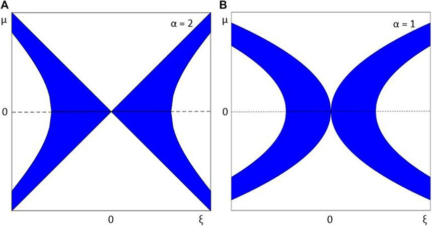
FIGURE 1. Instability region (blue) for case 2, β > 0, γ > 0; α = 2 (A), α = 1 (B).

FIGURE 2

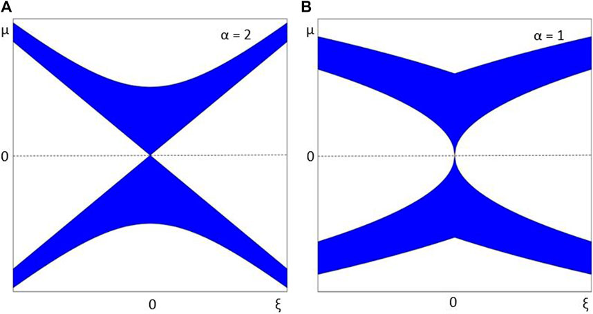
FIGURE 2. Instability region (blue) for case 3, β > 0, γ < 0; α = 2 (A), α = 1 (B).

FIGURE 3

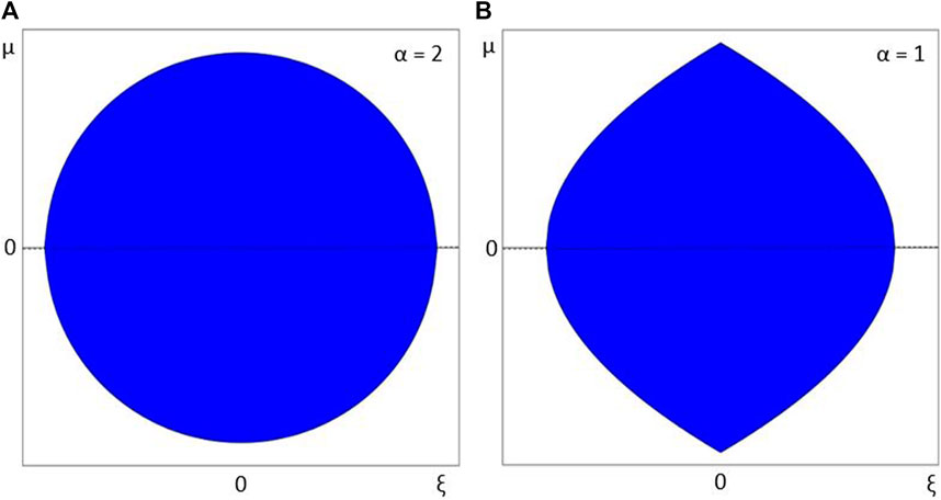
FIGURE 3. Instability region (blue) for case 4, β < 0, γ < 0; α = 2 (A), α = 1 (B).

3 Beyond linear stability: Numerical results

To numerically validate the regions defined earlier as well as to explore the extended behavior of perturbations in the unstable region, we adopt a numerical method proposed in Kirkpatrick and Zhang (2016) to handle the fractional Laplacian. The method splits the operator and uses the Fourier pseudospectral method to advance the fractional and integer derivatives. The nonlinearity is integrated exactly, and the two components are then coupled back together with the second-order Strang method (Strang, 1968). The method is explicit and has high order spatial accuracy and little computational cost. To extend the method from Kirkpatrick and Zhang (2016) to integrate Eq. 2, we increase the dimension of the domain by one and integrate the second derivative in t in the same step as the fractional Laplacian in Fourier space.

The two-dimensional computational domain for the problem is defined to be Ω = [a, b] × [t_a, t_b]. Let J and R be positive even integers with the fractionality parameter α ∈ [0, 2]. Define the mesh sizes h_x = (b − a)/J and h_t = (t_b − t_a)/R and grid points x_j = a + jh_x for 0 ≤ j < J, and t_r = t_a + rh_t for 0 ≤ r < R. The outline to advance a state from ψ(z_n) to ψ(z_n+1) is as follows:

${\psi }_{r,j}^{\left(1\right)}={\psi }_{r,j}^n\exp \left\{-i\frac{k}{2}\gamma |{\psi }_{r,j}^n{|}^2\right\},,(15)$

${\psi }_{r,j}^{\left(2\right)}=\sum _{m=-R/2}^{R/2-1}\sum _{l=-J/2}^{J/2-1}{\widehat{\psi }}_{m,l}^{\left(1\right)}\exp \left\{-ik\left(|{\xi }_l{|}^{\alpha }+\beta {\mu }_m^2\right)\right\},(16)$

$\ast \exp \left\{i\left[{\xi }_l\left(x_j-a\right)+{\mu }_m\left(t_r-t_a\right)\right]\right\},,(17)$

${\psi }_{r,j}^{n+1}={\psi }_{r,j}^{\left(2\right)}\exp \left\{-i\frac{k}{2}\gamma |{\psi }_{r,j}^{\left(2\right)}{|}^2\right\},(18)$

Where ${\psi }_j^n$ denotes the numerical approximation of ψ(x_j, t_r), k is the step size in z, and $\widehat{\psi }$ is the two-dimensional Fourier transform of ψ in x and t. The frequencies in x and t are given by ${\xi }_l=\frac{2l\pi }{b-a}$ for − J/2 ≤ l ≤ J/2–1 and ${\mu }_m=\frac{2m\pi }{t_b-t_a}$ for − R/2 ≤ m ≤ R/2–1, respectively. An alternative method that has been shown to integrate the FNSE is known as the split-step Galerkin method (Wang et al., 2019). This method also employs the second-order Strang split-step method for splitting the potential and nonlinear operators; however, it uses the Legendre spectral Galerkin method for approximating the Riesz space-fractional derivative.

As expected, starting conditions from the stable region do not grow and either remain the same or travel along the domain in all cases. On the other hand, Figure 4 shows a breather emerging from the MI region for α = 1. The initial perturbed mode grows in amplitude until reaching some upper bound before returning and repeating this process. Higher order modes are also excited. Figure 5 shows the evolution of the lowest mode from the breather in Figure 4 for various α. The different lines represent α = 2.0, 1.5, 1.0, and 0.5 with respective values of λ² ≈ − 0.79, −0.68, −0.5, and −0.16. We can see from Eq. 9 that as the imaginary part of λ increases, the amplitude grows much faster. We search for patterns in the behavior as α is decreased to see if the nonlocal operator plays any special part; however, no definitive conclusion can be reached. Since the modes move to nearly identical heights, we can confirm that this forms a breather. This was further confirmed in the behavior of the power spectrum. This kind of response was seen for all the points sampled from the focusing case β = γ = −1. If the signs of the derivatives in x and t are opposite, the behavior is more erratic. It is important to note that due to the numerical method requiring periodic boundaries, only integer multiple modes appear in our simulation.

FIGURE 4

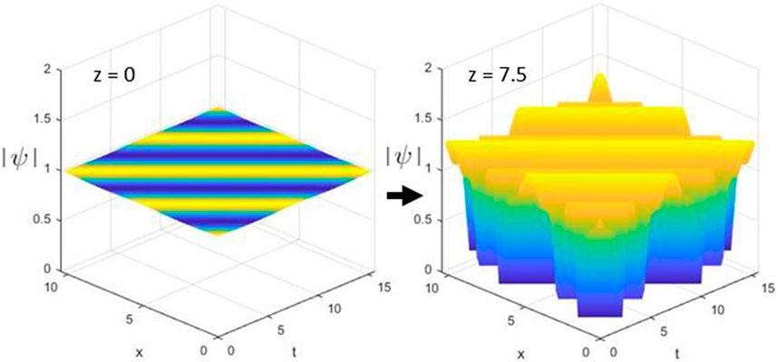
FIGURE 4. Appearance of a breather from the MI region, α = 1.

FIGURE 5

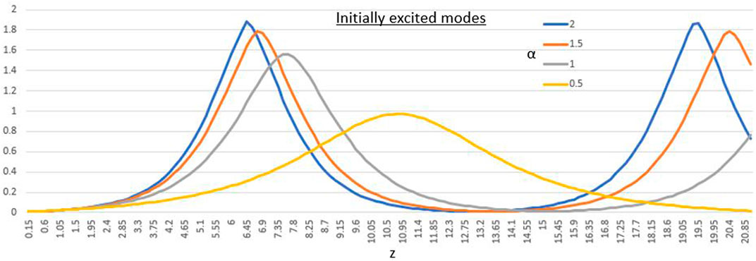
FIGURE 5. Evolution of the amplitude for the first excited mode (ξ = 0.5, μ = 1.1, γ = 1, and β = 1).

4 Existence of ground states

In this section, we adopt a numerical method proposed in the study by Duo and Zhang (2015) called the fractional gradient flow with discrete normalization (FGFDN) which is designed to find the ground and first excited states of the fractional Schrödinger equation in an infinite potential well. In physics literature, the eigenfunctions that satisfy the equation Lψ = λψ are commonly called the stationary states, and the eigenfunction corresponding to λ = 0 is referred to as the ground state. The eigenvalues and eigenfunctions can be found exactly in the linear non-fractional case (Greiner, 2001; Bao et al., 2007). However, the fractional case presents new challenges, and there are few results available for either the linear or nonlinear case. The numerical results given by Duo and Zhang et al. (2015) for the linear case show that the nonlocal interactions from the fractional Laplacian lead to a large scattering inside the potential well. Furthermore, a decrease in α leads to stronger scattering. In the nonlinear case, the local interactions generate boundary layers in the ground states, with the first excited states also forming inner layers.

The method used here is analogous to the normalized gradient flow used to find stationary states of the standard Schrödinger equation. The authors Duo and Zhang (2015) present a novel semi-discretization of the fractional gradient flow and the fractional operator can be transformed into a symmetric Toeplitz matrix.

In our adaptation, we increase the dimension by one and add the central finite difference to account for the temporal dispersion. We add an infinite potential term to Eq. 1, where the potential V(x, t) is designed to be infinite outside our numerical domain, Ω, and equal to zero for points located inside Ω.

$i\frac{\partial \psi }{\partial z}+{\left(-{\mathrm{\Delta }}_x\right)}^{\alpha /2}\psi +\beta \frac{{\partial }^2\psi }{\partial t^2}+\gamma |\psi {|}^2\psi +V\left(x,t\right)\psi =0.(19)$

Herein, we will define the Riesz fractional Laplacian (−Δ)^α/2 through the principal value integral (Samko et al., 1993; Valdinoci, 2009; Du et al., 2012).

${\left(-\mathrm{\Delta }\right)}^{\alpha /2}\psi \left(x\right)=C_{1,\alpha }\int \frac{\psi \left(x\right)-\psi \left(y\right)}{|x-y{|}^{1+\alpha }}dy,(20)$

where the normalization constant is given by C_1,α = Γ(1 + α) sin(απ/2)/π and the function Γ(z) represents the gamma function. Alternative methods have been proposed that are based on the pseudo-differential representation given as $-{(-\mathrm{\Delta })}^{\alpha /2}\psi (x)={\mathcal{F}}^{-1}[-|\xi {|}^{\alpha }\mathcal{F}(\psi )]$, where $\mathcal{F}$ is the Fourier transform and ξ is the wave number in x. The validity of these methods is still under consideration (Laskin, (2000c; Guo and Xu, 2006; Dong and Xu, 2007). By using the principal value integral representation, we are assured to capture the effects from the nonlocal interactions.

To find the stationary states, we assume an ansatz for the wave function as

$\psi \left(x,t,z\right)=e^{-i\mu z}\varphi \left(x,t\right),x,z\in \mathbb{R},t\ge 0,(21)$

where $\mu \in \mathbb{R}$. Substituting (21) into (19) and using the mass conservation constraint, we arrive at the eigenvalue equation as follows:

$\mu \varphi \left(x,t\right)=\left[{\left(-{\mathrm{\Delta }}_x\right)}^{\alpha /2}-\beta \frac{{\partial }^2}{\partial t^2}-\gamma |\varphi {|}^2-V\left(x,t\right)\right]\varphi ,,(22)$

$\Vert \varphi {\Vert }^2=\iint |\varphi \left(x,t\right){|}^{2}dxdt=1.(23)$

Due to the infinite well potential imposing V(x, t) = ∞ outside of Ω, the problem is reduced to finding the eigenfunction satisfying (22) and (23) within Ω and that ϕ(x, t) = 0 for $(x,t)\in \mathbb{R}\times \mathbb{R}\backslash \mathrm{\Omega }$. We can use the constraint of Eq. 23 to recover the corresponding eigenvalue after finding the eigenfunction by

$\mu =\iint {\varphi }^{\ast }{\left(-\mathrm{\Delta }\right)}^{\alpha /2}\varphi -\beta {\varphi }^{\ast }\frac{{\partial }^2\varphi }{\partial t^2}-\gamma |\varphi {|}^{4}dxdt.(24)$

For the one-dimensional linear Schrödinger equation (without the time dispersion) using the classical Laplacian (α = 2) in the infinite well potential, the eigenvalues and eigenfunctions can be found exactly (Greiner, 2001; Laskin, 2000a). For the nonlinear case, γ ≠ 0, the eigenvalue problem cannot be solved exactly; however, the solutions to the linear case give a good approximation for the weakly nonlinear regime when γ is o(1). For the strongly defocusing case, γ ≫ 1, the leading order approximation can be found through the Thomas–Fermi approximation (Zhang, 2006; Bao et al., 2007). When dealing with the fractional version, Bañuelos (Banuelos and Kulczycki, 2004) provided an approximation of the lower and upper bounds for the smallest eigenvalue in the linear case for α ∈ (0, 2]. A more general estimate is later given in DeBlassie (2004) and Chen and Song (2005) for all eigenvalues. Kwaśnicki (2010) then found asymptotic approximations to all eigenvalues in the linear case in a bounded domain. Laskin has provided asymptotic approximations for the s-th eigenvalue of the linear FSE (Laskin, 2000b). We will focus on finding the eigenfunctions and eigenvalues of Eqs 22 and 23.

Since we are searching for the stationary states, we discretize the operator on the right of Equation 22 (subject to constraint 23) and numerically propagate the equation until it levels off and successive iterations no longer change the solution by more than some small required value. Through a change of variables, we can rewrite the principal value integral (20) and then set up the equation as

$\begin{array}{ll}\hfill \frac{\partial \varphi }{\partial z}& =C_{1,\alpha }{\int }_0^{\infty }\frac{\varphi \left(x-\xi ,t,z\right)-2\varphi \left(x,t,z\right)+\varphi \left(x+\xi ,t,z\right)}{{\xi }^{1+\alpha }}d\xi \hfill \\ \hfill & -\frac{{\partial }^2\varphi }{\partial t^2}-\gamma |\varphi {|}^2\varphi .\hfill \end{array}(25)$

Since ϕ = 0 outside of Ω, the nonlocal component of the wave function will only interact with other points inside Ω and the operator can be discretized as shown in Duo and Zhang (2015) with the addition of the central finite difference accounting for the second partial derivative in t.

The initial profile may be given as the 0^th eigenfunction of the standard linear Schrödinger equation. We assume this is a good starting point with the idea being that the eigenfunction for the fractional version is not very different. We use the function:

$\varphi \left(x,t,0\right)=\frac{1}{L}\sin \left[\frac{\pi }{2}\left(1+\frac{x}{L}\right)\right]\sin \left[\frac{\pi }{2}\left(1+\frac{t}{L}\right)\right],(26)$

where the domain is defined by x ∈ [ − L, L] and t ∈ [ − L, L].

Figure 6 shows the wave function of the ground states in an infinite potential well for the linear case (top row) and nonlinear case (bottom row) for three different values of α (left to right). The wave function is always symmetric about the x or t axis with respect to the center of the infinite potential well. As the fractional parameter is decreased from 2 to 0, we see boundary layers emerge for α when it is small and the layers are more discernible when γ is large. In contrast to the one-dimensional case from Duo and Zhang (2015), the boundary layers are not very noticeable for α near 2.

FIGURE 6

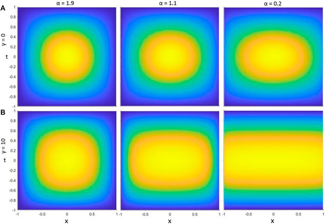
FIGURE 6. Ground states of the fractional Schrödinger equation with temporal dispersion. Results for the linear equation are in (A), while the results of the nonlinear equation are in (B).

We also see the peak amplitude decrease from 0.986 to 0.847 in the linear case as α decreases from 1.9 to 0.2. The peak amplitudes for the nonlinear case are also low and decrease from 0.848 to 0.675.

Our analysis extends the nonlinear parameter to γ = 10. To have a physical interpretation of this constant, we relate to the work in the study by Grynko et al. (2018) as an example where peak intensities reached I ∼ 1.2 × 10¹²W/cm² and a nonlinear refractive index coefficient of n₂ ∼ 7 × 10⁻¹⁵ cm²/W. Multiplying these together gives the nondimensional constant $\sim 10^{-2}$. Our numerical results with the nonlinear refractive index of γ = 10 give peak amplitudes of 0.85. By squaring and multiplying by γ, we have 0.85² × 10 = 7.225.

Table 1 shows the calculated eigenvalues recovered through Eq. 24. We see that in the linear case, as α → 0, the eigenvalue approaches π²/4 (the eigenvalue of the one-dimensional standard Schrödinger equation). Similarly, as α → 2, the eigenvalue approaches π²/2 (the eigenvalue of the two-dimensional standard Schrödinger equation).

TABLE 1

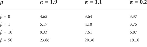
TABLE 1. Eigenvalues of the ground states of the fractional Schrödinger equation with quadratic dispersion in an infinite potential well.

5 Dynamics of collapse

In this section, we center our attention on the behavior when the self-focusing nonlinearity is the driving force toward a collapse. An interesting feature observable in the FNSE is that as α → 0, Eq. 1 approaches the integrable one-dimensional NLSE, and when α → 2, Eq. 1 approaches the two-dimensional NLSE. This section explores the phenomena exhibited throughout the full range of α ∈ (0, 2). Before we embark in the dynamics at high intensities, we should highlight that one can rigorously show the existence of the evolving field for low amplitude initial conditions (Choi and Aceves, 2022).

Using the propagation numerical method mentioned in Section 2, we provide the simulation with an initial field profile of $\psi (x,t,0)=A{e}^{-x^2-t^2}$. The first interesting result is the minimal value of A, where the maximum modulus of ψ(x, t), located at (x = 0, t = 0), does not initially decrease. In other words, we search for the point where we see the first occurrence of the positive self-focusing effect. This happens at A ≈ 1.333 for α ≈ 1.36 as shown in Figure 7. The figure measures the distance propagated before max|ψ| decreases, and the various lines represent different starting conditions. The horizontal axis represents α between 0 and 2. The contraction from the focusing only lasts for a brief moment in z after which the field diffracts and disperses. As A is increased, more values of α above and below 1.36 also see a similar contraction.

FIGURE 7

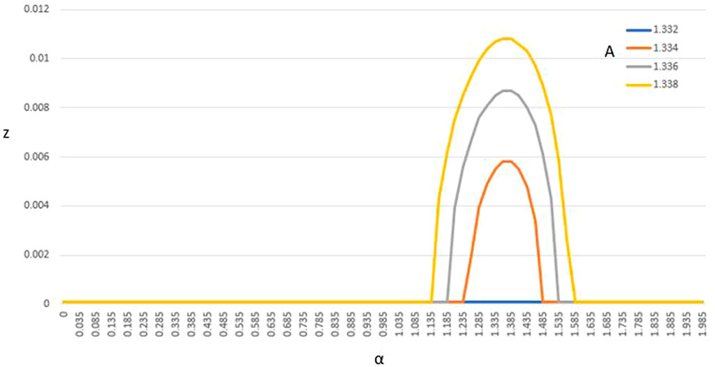
FIGURE 7. Measuring the length of propagation in z before the maximum value of |ψ| begins to decrease. The first appearance of the field contracting is seen at A ≈ 1.333 for α ≈ 1.36.

This behavior continues as A increases, and the first appearance of the field collapsing to a single point is at A ≈ 2 with α ≈ 0.96. This point is represented by the blue spike shown in Figure 8. In this section, we classify the field as a collapse if the full width at half maximum (FWHM) measurement is reduced to three grid points or below in either dimension. As A is increased further, the spike that shows the largest α that incurs a blowup increases and also happens at a lower value of z. At A = 2.75, the solution now collapses for the standard Laplacian (α = 2). Around A = 2.75, the spike on the left has shifted down to its minimum value before it changes direction and begins to increase to the right. Subsequently, higher values of A continue to shift this spike to the right and the corresponding z decreases.

FIGURE 8

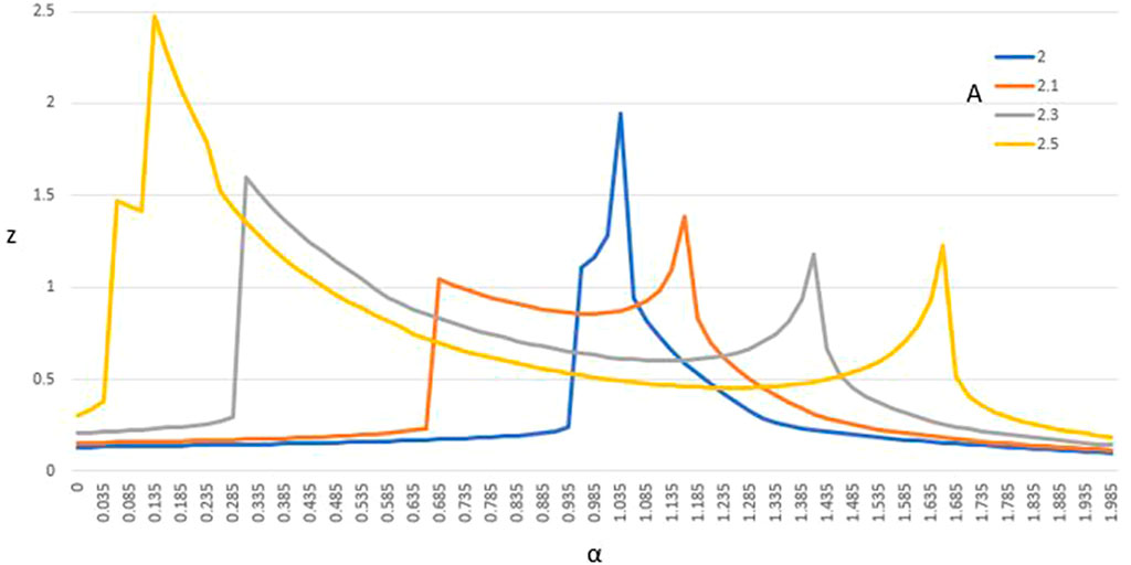
FIGURE 8. Measuring the length of propagation in z before the maximum value of |ψ| begins to decrease. The first collapse of the field is seen at the blue spike at A ≈ 2 for α ≈ 0.96.

A well-known feature of solutions with singularities for the NLS with the standard Laplacian is that the self-focusing effect causes the amount of power that goes into the singularity to always be equal to the critical power needed for blowup (Fibich and Papanicolaou, 1999). It is also shown that for cases where the initial profile is not radially symmetric when the field is near the point of collapse, the field approaches a radially symmetric asymptotic profile (Aceves et al., 1995). In this section, we show numerically that the same phenomenon does not hold when the degree of fractionality in one dimension is lowered. However, as the strength of the nonlinearity is increased, the field approaches symmetry again at the moment of collapse.

Figure 9 displays an example of an initial profile that starts radially symmetric in x and t although collapses asymmetrically. The field is of critical power to cause a collapse and α = 1. As the profile coalesces toward the center, we first notice the width in t shrinks first. After which, the width in x shrinks and becomes thinner than that in t until the blowup occurs. A more detailed evolution of the field can be seen in Figure 10, where the full width at half maximum in x and t is measured as the field propagates, shown in blue and orange, respectively. The maximum modulus is shown in grey and plotted on the right axis. We can see the field trending toward a collapse on the right and a gap between the two widths appears through to the final collapse. This same gap is present even if the initial condition is not symmetric but rather wide in x or t.

FIGURE 9

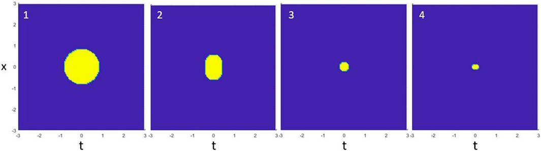
FIGURE 9. Collapse event for α = 1. The profile is not radially symmetric.

FIGURE 10

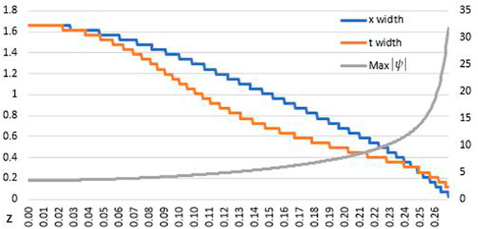
FIGURE 10. Collapse event for α = 1. The profile is not radially symmetric.

In an effort to measure the gap dependence on α and the power, Figure 11 measures the maximum ratio of the widths near the point of blowup. We see that lower power profiles enable a larger separation, while higher power profiles prevent the separation from growing. At higher power levels, the nonlinearity becomes the driving force that pushes the profile toward symmetry. As α approaches 2, we see the field move toward symmetry as expected. Power levels of A = 7.5 and A = 10 were also simulated, and these resulted in symmetry at the moment of collapse. We will also note that even though the field becomes symmetric at the end, there are fluctuations in the shape throughout the simulation.

FIGURE 11

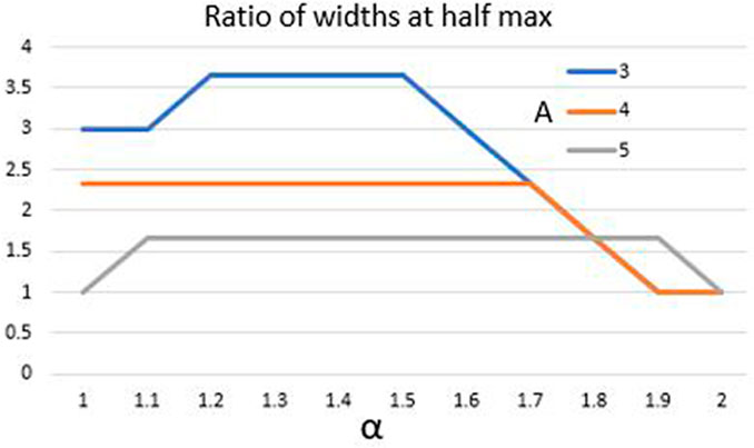
FIGURE 11. Measuring the maximum of the ratio of widths near blowup. Each line represents a different initial condition with varying A. Increasing the power brings the field closer to symmetric.

Values of α < 1 are not included since whether or not the field collapses are uncertain. Figure 12 shows an example of the cross-section evolution of a breather profile when α = 0.3. Herein, the profile actually splits into three different peaks that remain near the center. The peak height rises and falls; however, it does not appear to collapse to a single point. Figure 13 shows the detailed evolution of each FWHM measurement and peak amplitude.

FIGURE 12

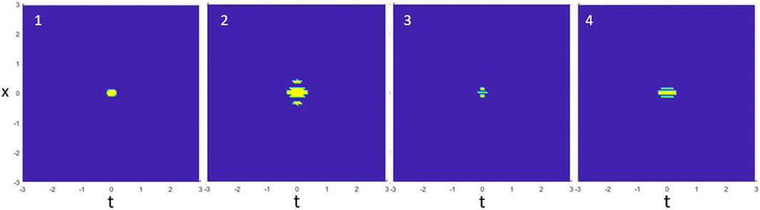
FIGURE 12. Example of the cross-section propagation for α = 0.3. The profile splits into three separate peaks, and the shape fluctuates without collapsing.

FIGURE 13

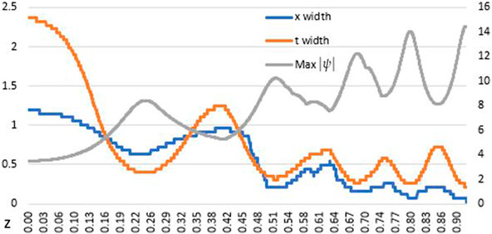
FIGURE 13. Example of the field propagation for α = 0.3. The profile does not collapse and a breather-like procession emerges.

6 Conclusion

We have proposed a model for short pulse propagation inspired by a laser cavity design that produces fractional diffraction in the presence of nonlinearity. This model generates new dynamics as we study mixed fractional/integer ordered operator equations. We have presented an exploration of the stability and spatio-temporal dynamics of the FNSE with quadratic temporal dispersion. The regions of modulational instability have been established given a continuous wave solution. The defocusing case is found to be in agreement with the standard NLSE in which it is always stable. Two previous numerical methods that describe the behavior during propagation and find the ground states have been extended to incorporate the quadratic dispersion. From the propagation method, we find that a breather emerges from the MI region. Using the FGFDN, we find the boundary layers are present when x is near the boundary for α being small, similar to the one-dimensional case. We have also analyzed the delicate balance between the diffraction/dispersion and the focusing nonlinearity. Given that the fractional derivative is only on the spatial x variable, the field is not radially symmetric near blowup. Approximate minimal power thresholds are found that cause the field to first contract through focusing as well as those that cause a blowup. Propagation of symmetric and non-symmetric initial conditions are investigated, and we study the ratio of widths at half maximum. A radially symmetric blowup is approached as the power is increased, and we shift it into a stronger nonlinear regime.

Data availability statement

The original contributions presented in the study are included in the article/Supplementary material; further inquiries can be directed to the corresponding author.

Author contributions

AA defined the main research topics to be studied and provided guidelines on the theoretical part. He was in charge of the preparation of the manuscript. AC did all numerical simulations and theoretical calculations.

Funding

Both authors’ work is supported by the U.S. National Science Foundation under the grant DMS-1909559.

Acknowledgments

AA wants to thank Dr. Brian Choi for useful discussions relevant to this work.

Conflict of interest

Author AC is employed at CitiBank.

The remaining authors declare that the research was conducted in the absence of any commercial or financial relationships that could be construed as a potential conflict of interest.

Publisher’s note

All claims expressed in this article are solely those of the authors and do not necessarily represent those of their affiliated organizations, or those of the publisher, the editors, and the reviewers. Any product that may be evaluated in this article, or claim that may be made by its manufacturer, is not guaranteed or endorsed by the publisher.

References

Aceves, A. B., Luther, G. G., De Angelis, C., Rubenchik, A. M., and Turitsyn, S. K. (1995). Energy localization in nonlinear fiber arrays: Collapse-effect compressor. Phys. Rev. Lett. 75, 73–76. doi:10.1103/PhysRevLett.75.73

PubMed Abstract | CrossRef Full Text | Google Scholar

Antoine, X., Tang, Q., and Zhang, Y. (2016). On the ground states and dynamics of space fractional nonlinear Schrödinger/Gross-Pitaevskii equations with rotation term and nonlocal nonlinear interactions. J. Comput. Phys. 325, 74–97. doi:10.1016/j.jcp.2016.08.009

CrossRef Full Text | Google Scholar

Banuelos, R., and Kulczycki, T. (2004). The Cauchy process and the Steklov problem. J. Funct. Analysis 211, 355–423. doi:10.1016/j.jfa.2004.02.005

CrossRef Full Text | Google Scholar

Bao, W., Lim, F. Y., and Zhang, Y. (2007). Energy and chemical potential asymptotics for the ground state of Bose-Einstein condensates in the semiclassical regime

Google Scholar

Chen, M., Wang, H., Ye, H., Huang, X., Liu, Y., Hu, S., et al. (2021a). Collapse arrest in the space-fractional Schrödinger equation with an optical lattice. Chin. Phys. B 30, 104206. doi:10.1088/1674-1056/abefc8

CrossRef Full Text | Google Scholar

Chen, M., Zeng, S., Lu, D., Hu, W., and Guo, Q. (2018). Optical solitons, self-focusing, and wave collapse in a space-fractional Schrödinger equation with a kerr-type nonlinearity. Phys. Rev. E 98, 022211. doi:10.1103/PhysRevE.98.022211

PubMed Abstract | CrossRef Full Text | Google Scholar

Chen, W., Wang, T., Wang, J., and Mu, Y. (2021b). Dynamics of interacting airy beams in the fractional Schrödinger equation with a linear potential. Opt. Commun. 496, 127136. doi:10.1016/j.optcom.2021.127136

CrossRef Full Text | Google Scholar

Chen, Z.-Q., and Song, R. (2005). Two-sided eigenvalue estimates for subordinate processes in domains. J. Funct. Analysis 226, 90–113. doi:10.1016/j.jfa.2005.05.004

CrossRef Full Text | Google Scholar

Choi, B., and Aceves, A. (2022). Well-posedness of the mixed-fractional nonlinear Schrödinger equation on R2. Partial Differ. Equations Appl. Math. 6, 100406. doi:10.1016/j.padiff.2022.100406

CrossRef Full Text | Google Scholar

DeBlassie, R. (2004). Higher order PDEs and symmetric stable processes. Probab. Theory Relat. Fields 129, 495–536. doi:10.1007/s00440-004-0347-x

CrossRef Full Text | Google Scholar

Dong, J., and Xu, M. (2007). Some solutions to the space fractional Schrödinger equation using momentum representation method. J. Math. Phys. 48, 072105. doi:10.1063/1.2749172

CrossRef Full Text | Google Scholar

Du, Q., Gunzburger, M., Lehoucq, R. B., and Zhou, K. (2012). Analysis and approximation of nonlocal diffusion problems with volume constraints. SIAM Rev. Soc. Ind. Appl. Math. 54, 667–696. doi:10.1137/110833294

CrossRef Full Text | Google Scholar

Duo, S., and Zhang, Y. (2015). Computing the ground and first excited states of the fractional Schrödinger equation in an infinite potential well. Commun. Comput. Phys. 18, 321–350. doi:10.4208/cicp.300414.120215a

CrossRef Full Text | Google Scholar

Fall, M. M., Mahmoudi, F., and Valdinoci, E. (2015). Ground states and concentration phenomena for the fractional Schrödinger equation. Nonlinearity 28, 1937–1961. doi:10.1088/0951-7715/28/6/1937

CrossRef Full Text | Google Scholar

Fibich, G., and Papanicolaou, G. (1999). Self-focusing in the perturbed and unperturbed nonlinear Schrödinger equation in critical dimension. SIAM J. Appl. Math. 60, 183–240. doi:10.1137/S0036139997322407

CrossRef Full Text | Google Scholar

Greiner, W. (2001). Quantum mechanics: An introduction. Berlin Heidelberg: Springer-Verlag.

Google Scholar

Grynko, R. I., Nagar, G. C., and Shim, B. (2018). Wavelength-scaled laser filamentation in solids and plasma-assisted subcycle light-bullet generation in the long-wavelength infrared. Phys. Rev. A 98, 023844. doi:10.1103/PhysRevA.98.023844

CrossRef Full Text | Google Scholar

Guo, X., and Xu, M. (2006). Some physical applications of fractional Schrödinger equation. J. Math. Phys. 47, 082104. doi:10.1063/1.2235026

CrossRef Full Text | Google Scholar

Huang, C., and Dong, L. (2016). Gap solitons in the nonlinear fractional Schrödinger equation with an optical lattice. Opt. Lett. 41, 5636–5639. doi:10.1364/OL.41.005636

PubMed Abstract | CrossRef Full Text | Google Scholar

Huang, X., Deng, Z., and Fu, X. (2017). Dynamics of finite energy airy beams modeled by the fractional Schrödinger equation with a linear potential. J. Opt. Soc. Am. B B 34, 976–982. doi:10.1364/JOSAB.34.000976

CrossRef Full Text | Google Scholar

Jiao, R., Zhang, W., Dou, L., Liu, B., Zhan, K., and Jiao, Z. (2021). Nonlinear propagation dynamics of Gaussian beams in fractional Schrödinger equation. Phys. Scr. 96, 065212. doi:10.1088/1402-4896/abf57f

CrossRef Full Text | Google Scholar

Kirkpatrick, K., Lenzmann, E., and Staffilani, G. (2013). On the continuum limit for discrete NLS with long-range lattice interactions. Commun. Math. Phys. 317, 563–591. doi:10.1007/s00220-012-1621-x

CrossRef Full Text | Google Scholar

Kirkpatrick, K., and Zhang, Y. (2016). Fractional Schrödinger dynamics and decoherence. Phys. D. Nonlinear Phenom. 332, 41–54. doi:10.1016/j.physd.2016.05.015

CrossRef Full Text | Google Scholar

Kwaśnicki, M. (2010). Eigenvalues of the fractional Laplace operator in the interval. J. Funct. Analysis 262, 2379–2402. doi:10.1016/j.jfa.2011.12.004

CrossRef Full Text | Google Scholar

Laskin, N. (2000a). Fractals and quantum mechanics. Chaos. 10, 780–790. doi:10.1063/1.1050284

PubMed Abstract | CrossRef Full Text | Google Scholar

Laskin, N. (2000b). Fractional quantum mechanics. Phys. Rev. E 62, 3135–3145. doi:10.1103/PhysRevE.62.3135

PubMed Abstract | CrossRef Full Text | Google Scholar

Laskin, N. (2000c). Fractional quantum mechanics and Lévy path integrals. Phys. Lett. A 268, 298–305. doi:10.1016/S0375-9601(00)00201-2

CrossRef Full Text | Google Scholar

Laskin, N. (2002). Fractional schrödinger equation. Phys. Rev. E 66, 056108. doi:10.1103/physreve.66.056108

CrossRef Full Text | Google Scholar

Li, P., Li, R., and Dai, C. (2021). Existence, symmetry breaking bifurcation and stability of two-dimensional optical solitons supported by fractional diffraction. Opt. Express 29, 3193–3210. doi:10.1364/OE.415028

PubMed Abstract | CrossRef Full Text | Google Scholar

Lischke, A., Pang, G., Gulian, M., Song, F., Glusa, C., Zheng, X., et al. (2019). What is the fractional laplacian? A comparative review with new results. J. Comput. Phys. 404, 109009. doi:10.1016/j.jcp.2019.109009

PubMed Abstract | CrossRef Full Text | Google Scholar

Liu, S., Zhang, Y., Malomed, B. A., and Karimi, E. (2022). Experimental realisations of the fractional schrö dinger equation in the temporal domain. http//:arXiv/org/abs.2208.01128.

Google Scholar

Longhi, S. (2015). Fractional Schrödinger equation in optics. Opt. Lett. 40, 1117–1120. doi:10.1364/OL.40.001117

PubMed Abstract | CrossRef Full Text | Google Scholar

Ren, X., and Deng, F. (2022). Dynamics of two-dimensional multi-peak solitons based on the fractional Schrödinger equation. J. Nonlinear Opt. Phys. Mat. 31, 2250004. doi:10.1142/s0218863522500047

CrossRef Full Text | Google Scholar

Ren, X., Deng, F., and Huang, J. (2022). Families of fundamental solitons in the two-dimensional superlattices based on the fractional Schrödinger equation. Opt. Commun. 519, 128439. doi:10.1016/j.optcom.2022.128439

CrossRef Full Text | Google Scholar

Rüter, C. E., Makris, K. G., El-Ganainy, R., Christodoulides, D. N., Segev, M., and Kip, D. (2010). Observation of parity–time symmetry in optics. Nat. Phys. 6, 192–195. doi:10.1038/nphys1515

CrossRef Full Text | Google Scholar

Samko, S., Kilbas, A., Samko, I., and Marichev, O. (1993). Fractional integrals and derivatives: Theory and applications. Switzerland: Gordon and Breach Science Publishers.

Google Scholar

Segev, M., Silberberg, Y., and Christodoulides, D. N. (2013). Anderson localization of light. Nat. Photonics 7, 197–204. doi:10.1038/nphoton.2013.30

CrossRef Full Text | Google Scholar

Strang, G. (1968). On the construction and comparison of difference schemes. SIAM J. Numer. Anal. 5, 506–517. doi:10.1137/0705041

CrossRef Full Text | Google Scholar

Valdinoci, E. (2009). From the long jump random walk to the fractional Laplacian. Bol. Soc. Espanola Mat. Apl. SeMA 49.

Google Scholar

Wang, J., Jin, Y., Gong, X., Yang, L., Chen, J., and Xue, P. (2022). Generation of random soliton-like beams in a nonlinear fractional Schrödinger equation. Opt. Express 30, 8199–8211. doi:10.1364/oe.448972

PubMed Abstract | CrossRef Full Text | Google Scholar

Wang, Y., Mei, L., Li, Q., and Bu, L. (2019). Split-step spectral Galerkin method for the two-dimensional nonlinear space-fractional Schrödinger equation. Appl. Numer. Math. 136, 257–278. doi:10.1016/j.apnum.2018.10.012

CrossRef Full Text | Google Scholar

Wu, Z., Cao, S., Che, W., Yang, F., Zhu, X., and He, Y. (2020). Solitons supported by parity-time-symmetric optical lattices with saturable nonlinearity in fractional Schrödinger equation. Results Phys. 19, 103381. doi:10.1016/j.rinp.2020.103381

CrossRef Full Text | Google Scholar

Xin, W., Song, L., and Li, L. (2021). Propagation of Gaussian beam based on two-dimensional fractional Schrödinger equation. Opt. Commun. 480, 126483. doi:10.1016/j.optcom.2020.126483

CrossRef Full Text | Google Scholar

Yao, X., and Liu, X. (2018). Solitons in the fractional Schrödinger equation with parity-time-symmetric lattice potential. Photonics Res. 6, 875–879. doi:10.1364/PRJ.6.000875

CrossRef Full Text | Google Scholar

Zeng, L., Belić, M. R., Mihalache, D., Shi, J., Li, J., Li, S., et al. (2022). Families of gap solitons and their complexes in media with saturable nonlinearity and fractional diffraction. Nonlinear Dyn. 108, 1671–1680. doi:10.1007/s11071-022-07291-z

CrossRef Full Text | Google Scholar

Zhang, L., Li, C., Zhong, H., Xu, C., Lei, D., Li, Y., et al. (2016a). Propagation dynamics of super-Gaussian beams in fractional Schrödinger equation: From linear to nonlinear regimes. Opt. Express 24, 14406–14418. doi:10.1364/OE.24.014406

PubMed Abstract | CrossRef Full Text | Google Scholar

Zhang, L., Zhang, X., Wu, H., Li, C., Pierangeli, D., Gao, Y., et al. (2019). Anomalous interaction of airy beams in the fractional nonlinear Schrödinger equation. Opt. Express 27, 27936–27945. doi:10.1364/OE.27.027936

PubMed Abstract | CrossRef Full Text | Google Scholar

Zhang, Y., Liu, X., Belić, M. R., Zhong, W., Zhang, Y., and Xiao, M. (2015). Propagation dynamics of a light beam in a fractional Schrödinger equation. Phys. Rev. Lett. 115, 180403. doi:10.1103/PhysRevLett.115.180403

PubMed Abstract | CrossRef Full Text | Google Scholar

Zhang, Y. (2006). Mathematical analysis and numerical simulation for bose–einstein condensation. Queenstown: Ph.D. thesis, National University of Singapore.

Google Scholar

Zhang, Y., Wang, R., Zhong, H., Zhang, J., Belić, M. R., and Zhang, Y. (2017). Optical bloch oscillation and zener tunneling in the fractional Schrödinger equation. Sci. Rep. 7, 17872–17877. doi:10.1038/s41598-017-17995-7

PubMed Abstract | CrossRef Full Text | Google Scholar

Zhang, Y., Wu, Z., Ru, J., Wen, F., and Gu, Y. (2020). Evolution of the bessel–Gaussian beam modeled by the fractional Schrödinger equation. J. Opt. Soc. Am. B 37, 3414–3421. doi:10.1364/josab.399840

CrossRef Full Text | Google Scholar

Zhang, Y., Zhong, H., Belić, M. R., Ahmed, N., Zhang, Y., and Xiao, M. (2016b). Diffraction-free beams in fractional Schrödinger equation. Sci. Rep. 6, 23645. doi:10.1038/srep23645

PubMed Abstract | CrossRef Full Text | Google Scholar

Zhu, X., Yang, F., Cao, S., Xie, J., and He, Y. (2020). Multipole gap solitons in fractional Schrödinger equation with parity-time-symmetric optical lattices. Opt. Express 28, 1631–1639. doi:10.1364/OE.382876

PubMed Abstract | CrossRef Full Text | Google Scholar