Numerical simulations of scattering of light from two-dimensional rough surfaces using the reduced Rayleigh equation

1. Introduction

Wave scattering from rough surfaces is an old discipline which keeps attracting a great deal of attention from the scientific and technological community. Several important technologies in our society rely on such knowledge, with radar technology being a prime example. In the past, the interaction of light with rough surfaces was often considered an extra complication that had to be taken into account in order to properly interpret or invert scattering data. However, with the advent of nanotechnology, rough structures can be used to design novel materials with tailored optical properties. Examples include: metamaterials (Agranovich and Gartstein, 2006; Maradudin, 2011), photonic crystals (Joannopoulos et al., 2008), “spoof” or “designer” surface plasmons (Pendry et al., 2004), optical cloaking (Pendry et al., 2006; Schurig et al., 2006; Baumeier et al., 2009), and designer surfaces (Méndez et al., 2002; Maradudin et al., 2008). These developments have made it even more important to have available efficient and accurate simulation tools to calculate both the far- and near-field behavior of the scattered and transmitted fields for any frequency of the incident radiation, including potential resonance frequencies of the structure.

Lord Rayleigh was the first to perform systematic studies of wave scattering from rough surfaces when, in the late 1800's, he studied the intensity distribution of a wave scattered from a sinusoidal surface (Rayleigh, 1896, 1907). Several decades later Mandelstam (1913) studied light scattering from randomly rough surfaces, thereby initiating the field of wave scattering from surface disordered systems. Since the initial publication of these seminal works, numerous studies on wave scattering from randomly rough surfaces have appeared in the literature (Bass and Fuks, 1979; Ogilvy, 1991; Voronovich, 1999; Zayats et al., 2005; Nieto-Vesperinas, 2006; Maradudin, 2007; Simonsen, 2010b), and several new multiple scattering phenomena have been predicted and confirmed experimentally. These phenomena include the enhanced backscattering and enhanced transmission phenomena, the satellite peak phenomenon, and coherent effects in the intensity–intensity correlation functions (McGurn et al., 1985; Méndez and O'Donnell, 1987; Gu et al., 1991; Freilikher et al., 1994; West and O'Donnell, 1995; Simonsen, 2010b).

These studies, and the methods they use, can be categorized as either perturbative or purely numerical (and non-pertubative). While the former group of methods is mainly limited to weakly rough surfaces, and therefore have limited applicability, the latter group of methods can be applied to a wider class of surface roughnesses. Rigorous numerical methods can in principle be used to study the wave scattering from surfaces of any degree of surface roughness. Such simulations are routinely performed for systems where the interface has a one-dimensional roughness, i.e., where the surface structure is constant along one of the two directions of the mean plane (Maradudin et al., 1990; Simonsen, 2010b). However, for the practically more relevant situation of a two-dimensional rough surface, the purely numerical and rigorous methods are presently less used due to their computationally intensive nature. The reason for this complexity is the fact that for a randomly rough surface there is no symmetry or periodicity in the surface structure that can be used to effectively reduce the simulation domain. For a periodic surface, for instance, it is sufficient to simulate a single unit cell, while for a random surface the unit cell is in principle infinite.

A wide range of simulation methods are currently available for simulating the interaction of light with matter, including the finite-difference time-domain (FDTD) method (Taflove and Hagness, 2005), the finite-element method (FEM) (Volakis et al., 2001; Jin, 2002), the related surface integral equation techniques also known as the boundary element method (BEM) or the method of moments (MoM) (Harrington, 1993; Hackbush, 1995; Bonnet, 1999; Boyd, 2001; Simonsen et al., 2011), the reduced Rayleigh equation (RRE) technique (Brown et al., 1984; McGurn and Maradudin, 1996; Madrazo and Maradudin, 1997; Simonsen and Maradudin, 1999; Soubret et al., 2001a,b; Zayats et al., 2005; Simonsen, 2010a), and spectral methods (Boyd, 2001).

The FDTD and FEM methods discretize the whole volume of the simulation domain. Due to the complex and irregular shape of a (randomly) rough surface, it is often more convenient, and may give more accurate results (for the same level of numerical complexity) (Kern and Martin, 2009), to base numerical simulations on methods where only the surface itself needs to be discretized. This is the case, for example, for the surface integral technique and the RRE methods.

The RRE is an integral equation where the unknown is either the scattering amplitude or the transmission amplitude. In the former (latter) case, one talks about the RRE for reflection (transmission). For reflection this equation was originally derived by Brown et al. (1984), and subsequently by Soubret et al. (2001a,b). Later it has also been derived for transmission (Greffet, 1988; Maradudin, 2012) and film geometries (Soubret et al., 2001a; Leskova, 2010; Nordam et al., 2012b).

In the past, the surface integral technique has been used to study light scattering from two-dimensional randomly rough, perfectly conducting or penetrable surfaces (Simonsen et al., 2010a,b, 2011). However, to date, a direct numerical and non-perturbative solution of the two-dimensional RRE has not appeared in the literature, even if its one-dimensional analog has been solved numerically and has been used to study the scattering from, and transmission through, one-dimensional rough surfaces (Madrazo and Maradudin, 1997; Simonsen and Maradudin, 1999; Simonsen, 2010a). The lesson learned from the one-dimensional scattering studies reported by Madrazo and Maradudin (1997), Simonsen and Maradudin (1999), and Simonsen (2010a) is that simulations based on a direct numerical solution of the RRE may give accurate non-perturbative results for systems where alternative methods struggle to give the same level of accuracy. Moreover, the reduced Rayleigh method also requires less memory than the rigorous surface integral technique for the same surface dimensions and discretization.

The main aim of this paper is to present a numerical method and formalism for the solution of the two-dimensional RRE for reflection. While we exclusively consider reflection, the formalism for transmission will be almost identical, and the resulting equation will have a similar form as for reflection. Additionally, the equation for transmission or reflection for a film geometry, i.e., for a film of finite thickness on top of a substrate, where only one interface is rough, will also have a similar form. The method presented will be illustrated by applying it to the study of the scattering of p- or s-polarized light from two-dimensional metallic or dielectric media separated from vacuum by an isotropic or anisotropic randomly rough surface.

This paper is organized as follows: First, in section 2 we present the scattering geometry to be considered. We will then present some relevant scattering theory, including the RRE for the geometry under study (section 3), followed by a detailed description of how the equation can be solved numerically (section 4). Next, we will present some simulation results obtained by the introduced method and we compare such results to experimentally available scattering data (section 5). We then discuss some of the computational challenges of this method (section 6), and, finally, in section 7 we draw some conclusions.

2. Scattering Geometry

We consider a system where a rough surface separates two regions. Region 1 is assumed to be vacuum (ε₁ = 1), and region 2 is filled with a metal or dielectric characterized by a complex dielectric function ε₂(ω), where the angular frequency is ω = 2πc/λ, with λ being the wavelength of the incident light in vacuum and c the speed of light in vacuum. The height of the surface measured in the positive x₃ direction from the x₁ x₂-plane is given by the single-valued function x₃ = ζ(x_‖), where x_‖ = (x₁, x₂, 0), which is assumed to be at least once differentiable with respect to x₁ and x₂. Angles of incidence (θ₀, ϕ₀) and scattering (θ_s, ϕ_s) are defined positive according to the convention given in Figure 1.

FIGURE 1

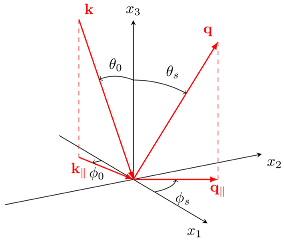
Figure 1. A sketch of the scattering geometry assumed in this work. The figure also shows the coordinate system used, angles of incidence (θ₀, ϕ₀) and scattering (θ_s, ϕ_s), and the corresponding lateral wavevectors k_‖ and q_‖, respectively.

In principle, the theory to be presented in section 3 can be used to calculate the scattering of light from any surface, provided it is not too rough. However, in this paper, we will consider randomly rough surfaces where ζ(x_‖) constitutes a stationary random process defined by

$\begin{array}{cc}\begin{array}{l}\langle \zeta \left(x_{\parallel }\right)\rangle =0,\\ \langle \zeta \left(x_{\parallel }\right)\zeta \left(x_{\parallel }{}^{\prime }\right)\rangle ={\delta }^{2}W\left(x_{\parallel }-x_{\parallel }{}^{\prime }\right)\text{},\end{array}& (1)\end{array}$

where the angle brackets denote an average over an ensamble of surface realizations. In writing Equation (1) we have defined the root-mean-square height of the surface, δ = 〈ζ²(x_‖)〉^1/2, and W(x_‖ − x_‖′) denotes the height-height auto-correlation function of the surface, normalized so that W(0) = 1 (Simonsen, 2010b). According to the Wiener–Khinchin theorem (Kampen, 2007), the power spectrum of the surface profile function is given by

$\begin{array}{cc}g\left(k_{\parallel }\right)={\displaystyle \int \text{}}{\text{d}}^2{x}_{\parallel }W\left(x_{\parallel }\right)\exp \left(-\text{i}{k}_{\parallel }·x_{\parallel }\right)\text{}.& (2)\end{array}$

The power spectra that will be considered in this work are of either the Gaussian form (Simonsen et al., 2011)

$\begin{array}{cc}g\left(k_{\parallel }\right)=\pi a_1{a}_2\exp \left(-\frac{k_1^2{a}_1^2}{4}-\frac{k_2^2{a}_2^2}{4}\right)\text{},& (3)\end{array}$

where a_i (i = 1, 2) denotes the lateral correlation length for direction i, or the cylindrical form (McGurn and Maradudin, 1996)

$\begin{array}{cc}g\left(k_{\parallel }\right)=\frac{4\pi }{k_{+}^2-k_{-}^2}\theta \left(k_{\parallel }-k_{-}\right)\theta \left(k_{+}-k_{\parallel }\right),& (4)\end{array}$

where k_‖ = |k_‖|, θ denotes the Heaviside unit step function, and k_± are wavenumber cutoff parameters, with k₋ < k₊. The cylindrical form in Equation (4) is a two-dimensional generalization of the power spectrum used in the experiments where West and O'Donnell confirmed the existence of the enhanced backscattering phenomenon for weakly rough surfaces (West and O'Donnell, 1995).

3. Scattering Theory

We consider a linearly p- or s-polarized plane wave which is incident on the surface from region 1, with the electric field given by E⁽⁰⁾(x; t) = E⁽⁰⁾(x|ω) exp(−iωt) where

$\begin{array}{cc}{E}^{(\text{0})}(x|\omega )={ℰ}^{(\text{0})}\left(k_{\parallel }\right)\exp \left[\text{i}{k}_{\parallel }·x_{\parallel }-\text{i}{\alpha }_1\left(k_{\parallel }\right)x_3\right]\text{},& (5\text{a})\end{array}$

with

$\begin{array}{cc}\begin{array}{l}{ℰ}^{(\text{0})}\left(k_{\parallel }\right)=-\frac{c}{\omega }\left[{\widehat{k}}_{\parallel }{\alpha }_1\left(k_{\parallel }\right)+{\widehat{x}}_3{k}_{\parallel }\right]{ℰ}_p^{(\text{0})}\left(k_{\parallel }\right)\\ +\left({\widehat{x}}_3\times {\widehat{k}}_{\parallel }\right){ℰ}_s^{(\text{0})}\left(k_{\parallel }\right)\text{},\end{array}& (5\text{b})\end{array}$

and

$\begin{array}{cc}{\alpha }_1\left(k_{\parallel }\right)={\left(\frac{{\omega }^2}{c^2}-k_{\parallel }^2\right)}^{\text{}1/2}\text{},\text{Re}{\alpha }_1\ge 0,\text{Im}{\alpha }_1\ge 0.& (5\text{c})\end{array}$

Here, and in the rest of the paper, a caret over a vector indicates a unit vector. The expressions in front of the amplitudes ℰ⁽⁰⁾_α(k_‖) (α = p, s) in Equation (5b) correspond to unit polarization vectors for incident light of linear polarization α. Moreover, k_‖ = (k₁, k₂, 0) denotes the lateral component of the wave vector $k=k_{\parallel }-{\alpha }_1(k_{\parallel }){\widehat{x}}_3$. When the lateral wavenumber of the incident field satisfies k_‖ ≤ ω/c, as will be assumed here, k_‖ is related to the angles of incidence according to

$\begin{array}{cc}{k}_{\parallel }=\frac{\omega }{c}\sin {\theta }_0\left(\cos {\varphi }_0,\sin {\varphi }_0,0\right)\text{},& (6)\end{array}$

where θ₀ and ϕ₀ are the polar and azimuthal angles of incidence, respectively (Figure 1). When writing the field of incidence, E⁽⁰⁾(x; t), a time harmonic dependence of the form exp(−iωt) was assumed. A similar time dependence will be assumed for all field expressions, but not indicted explicitly.

Above the surface roughness region, i.e., for x₃ > max ζ(x_‖), the scattered field can be written as a superposition of upwards propagating reflected plane waves:

$\begin{array}{cc}{E}^{(\text{s})}(x|\omega )\text{}=\text{}{\displaystyle \int \frac{{\text{d}}^2{q}_{\parallel }}{{\left(2\pi \right)}^2}}{ℰ}^{(\text{s})}\left(q_{\parallel }\right)\exp \left[\text{i}{q}_{\parallel }·x_{\parallel }+\text{i}{\alpha }_1\left(q_{\parallel }\right)x_3\right]\text{},& (7\text{a})\end{array}$

where

$\begin{array}{cc}{ℰ}^{(\text{s})}\left(q_{\parallel }\right)=\frac{c}{\omega }\left[{\widehat{q}}_{\parallel }{\alpha }_1\left(q_{\parallel }\right)-{\widehat{x}}_3{q}_{\parallel }\right]{ℰ}_{\text{p}}^{(\text{s})}\left(q_{\parallel }\right)+\left({\widehat{x}}_3\times {\widehat{q}}_{\parallel }\right){ℰ}_{\text{s}}^{(\text{s})}\left(q_{\parallel }\right).& (7\text{b)}\end{array}$

The integration in Equation (7a) is over the entire q_‖-plane, including the evanescent region q_‖ > ω/c. Therefore, both propagating and evanescent modes are included in E^(s)(x|ω).

We will assume that a linear relationship exists between the amplitudes of the incident and the scattered fields, and we write (for α = p, s)

$\begin{array}{cc}{ℰ}_{\alpha }^{{}^{(\text{s})}}\left(q_{\parallel }\right)={\displaystyle \sum _{\beta =\text{p},\text{s}}{R}_{\alpha \beta }}\left(q_{\parallel }|k_{\parallel }\right){ℰ}_{\beta }^{(0)}\left(k_{\parallel }\right).& (8)\end{array}$

Here we have introduced the so-called scattering amplitude R_αβ(q_‖|k_‖), which describes how incident β-polarized light characterized by a lateral wave vector k_‖ is converted by the surface roughness into scattered light of polarization α and lateral wave vector q_‖. When q_‖ ≤ ω/c, the wave vector q_‖ is related to the angles of scattering (θ_s, ϕ_s) by

$\begin{array}{cc}{q}_{\parallel }=\frac{\omega }{c}\sin {\theta }_s\left(\cos {\varphi }_s,\sin {\varphi }_s,0\right)\text{}.& (9)\end{array}$

Below the surface region, i.e., for x₃ < min ζ(x_‖), the transmitted electric field can be written as

$\begin{array}{cc}\begin{array}{l}{E}^{(\text{t})}\left(x_{\parallel }|\omega \right)={\displaystyle \int \frac{{\text{d}}^2{p}_{\parallel }}{{(2\pi )}^2}}{ℰ}^{(\text{t})}\left(p_{\parallel }\right)\exp \left[\text{i}{p}_{\parallel }·x_{\parallel }-\text{i}{\alpha }_2\left(p_{\parallel }\right)x_3\right]\hfill \end{array}& (10\text{a})\end{array}$

with

$\begin{array}{cc}\begin{array}{l}{ℰ}^{(\text{t})}\left(p_{\parallel }\right)=-\frac{1}{\sqrt{{\epsilon }_2(\omega )}}\frac{c}{\omega }\left[{\widehat{p}}_{\parallel }{\alpha }_2\left(p_{\parallel }\right)+{\widehat{x}}_3{p}_{\parallel }\right]{ℰ}_p^{(\text{t})}\left(p_{\parallel }\right)\\ +\left({\widehat{x}}_3\times {\widehat{p}}_{\parallel }\right){ℰ}_s^{(\text{t})}\left(p_{\parallel }\right)\text{}.\end{array}& (10\text{b})\end{array}$

In writing Equation (10) we have introduced wave vectors of the transmitted field $p=p_{\parallel }-{\alpha }_{\text{2}}\left(p_{\parallel }\right){\widehat{x}}_3$, where

$\begin{array}{cc}{\alpha }_2\left(p_{\parallel }\right)={\left[{\epsilon }_2(\omega )\frac{{\omega }^2}{c^2}-p_{\parallel }^2\right]}^{1/2}\text{},\text{Re}{\alpha }_2\ge 0,\text{Im}{\alpha }_2\ge 0.& (11)\end{array}$

In complete analogy to what was done for reflection, a transmission amplitude T_αβ(p_‖|k_‖) may be defined via the following linear relation between the amplitudes of the incident and transmitted fields (α = p, s)

$\begin{array}{cc}{ℰ}_{\alpha }^{(\text{t})}\left(p_{\parallel }\right)={\displaystyle \sum _{\beta =\text{p},\text{s}}{T}_{\alpha \beta }}\left(p_{\parallel }|k_{\parallel }\right){ℰ}_{\beta }^{(\text{0})}\left(k_{\parallel }\right)\text{}.& (12)\end{array}$

Since the forms of the electric field given by Equations (5), (7), and (10) also are valid far away from the surface region, they are referred to as the asymptotic forms of the electric field. These equations automatically satisfy the boundary conditions at infinity.

In passing we note that once the incident field has been specified, the scattered and transmitted fields are fully specified outside the surface roughness region if the reflection [R_αβ(q_‖|k_‖)] and transmission [T_αβ(p_‖|k_‖)] amplitudes are known. We will now address how the reflection amplitude can be calculated.

3.1. The Rayleigh Hypothesis

Above the surface, i.e., in the region x₃ > max ζ(x_‖), the total electric field is equal to the sum of the incident and the scattered field, E⁽⁰⁾(x|ω) + E^(s)(x|ω). Below the surface, in the region x₃ < min ζ(x_‖), it equals the transmitted field, E^(t)(x|ω). In the surface roughness region, min ζ(x_‖) ≤ x₃ ≤ max ζ(x_‖), these forms of the total field will not generally be valid. In particular, when we are above the surface but still below its maximum point, i.e., ζ(x_‖) ≤ x₃ < max ζ(x_‖), the expression for the scattered field will also have terms containing exp[iq_‖ · x_‖ − iα₁(q_‖)x₃]. Similarly, the transmitted field in the surface region has to contain an additional term similar to Equation (10a) but with the exponential function replaced by exp[iq_‖ · x_‖ + iα₂(q_‖)x₃] (and a different amplitude).

If the surface roughness is sufficiently weak, however, the asymptotic form of the fields, Equations (5), (7), and (10), can be assumed to be a good approximation to the total electric field in the surface roughness region. This assumption is known as the Rayleigh hypothesis (Rayleigh, 1896, 1907; Maradudin, 2007), in honor of Lord Rayleigh, who first used it in his seminal studies of wave scattering from sinusoidal surfaces (Rayleigh, 1896, 1907). For a (one-dimensional) sinusoidal surface, x₃ = ζ₀sin(Λ x₁), the criterion for the validity of the Rayleigh hypothesis, and thus equations that can be derived from it (like the RRE to be introduced below), is known to be ζ₀Λ < 0.448, independent of the wavelength of the incident light (Millar, 1969, 1971). For a randomly rough surface, however, the absolute limit of validity of this hypothesis is not generally known, though some numerical studies have been devoted to finding the region of validity for random surfaces (Mainguy and Greffet, 1998; Tishchenko, 2009). Even if no absolute criterion for the validity of the Rayleigh hypothesis for randomly rough surfaces is known, it remains true that it is a small-slope hypothesis. In particular, if the randomly rough surface is characterized by an rms height δ, and a correlation length a [see section 2 and Simonsen (2010b) for details], there seems to be a consensus in the literature on the Rayleigh hypothesis being valid if δ/a ≪ 1 (Maradudin, 2007; Tishchenko, 2009). We stress that the validity of the Rayleigh hypothesis does not require the amplitude of the surface roughness to be small, only its slope.

3.2. The Reduced Rayleigh Equation

Under the assumption that the Rayleigh hypothesis is valid, the total electric field in the surface region, min ζ(x_‖) < x₃ < max ζ(x_‖), can be written in the form given by Equations (5), (7), and (10) [with Equations (8) and (12)]. Hence, these asymptotic fields can be used to satisfy the usual boundary conditions on the electromagnetic field at the rough surface x₃ = ζ(x_‖) (Jackson, 2007; Stratton, 2007). In this way, one obtains the so-called Rayleigh equations, a set of coupled inhomogeneous integral equations, which the reflection and transmission amplitudes should satisfy.

In the mid-1980's, it was demonstrated by Brown et al. (1984) that either the reflection or transmission amplitude could be eliminated from the Rayleigh equations, resulting in an integral equation for the remaining amplitude only. Since this latter integral equation contains only the field above (below) the rough surface, it has been termed the reduced Rayleigh equation for reflection (transmission). Subsequently, RREs for two-dimensional film geometries, i.e., a film of finite thickness on top of an infinitely thick substrate, where only one interface is rough, was derived by Soubret et al. (2001a,b) and Leskova (2010); (Nordam et al., 2012b). Moreover, RREs for reflection from clean, perfectly conducting, two-dimensional randomly rough surfaces (Nordam et al., 2012a) and RREs for transmission through clean, penetrable two-dimensional surfaces (Maradudin, 2012) have been derived.

For the purposes of the present study, we limit ourselves to a scattering system consisting of a clean, penetrable, two-dimensional rough surface x₃ = ζ(x_‖) (section 2). If the scattering amplitudes are organized as the 2 × 2 matrix

$\begin{array}{cc}R\left(q_{\parallel }|k_{\parallel }\right)=\left(\begin{array}{cc}{R}_{pp}(q_{\parallel }|k_{\parallel })& R_{ps}(q_{\parallel }|k_{\parallel })\\ R_{sp}(q_{\parallel }|k_{\parallel })& R_{ss}(q_{\parallel }|k_{\parallel })\end{array}\right)\text{},& (13)\end{array}$

the RRE (for reflection) for this geometry can be written in the form (McGurn and Maradudin, 1996; Soubret et al., 2001a,b)

$\begin{array}{cc}\begin{array}{l}{\displaystyle \int \frac{{\text{d}}^2{q}_{\parallel }}{{(2\pi )}^2}}\frac{I({\alpha }_{\text{2}}(p_{\parallel })-{\alpha }_{\text{1}}(q_{\parallel })|p_{\parallel }-q_{\parallel })}{{\alpha }_{\text{2}}(p_{\parallel })-{\alpha }_{\text{1}}(q_{\parallel })}{M}^{+}(p_{\parallel }|q_{\parallel })R(q_{\parallel }|k_{\parallel })\\ =-\frac{I({\alpha }_{\text{2}}(p_{\parallel })+{\alpha }_{\text{1}}(k_{\parallel })|p_{\parallel }-k_{\parallel })}{{\alpha }_{\text{2}}(p_{\parallel })+{\alpha }_{\text{1}}(k_{\parallel })}{M}^{-}(p_{\parallel }|k_{\parallel }),\end{array}& (14\text{a)}\end{array}$

where

$\begin{array}{cc}I\left(\gamma |Q_{\parallel }\right)={\displaystyle \int {\text{d}}^2}{x}_{\parallel }\exp \left[-\text{i}\gamma \zeta \left(x_{\parallel }\right)\right]\exp \left(-\text{i}{Q}_{\parallel }·x_{\parallel }\right),& (14\text{b)}\end{array}$

and

$\begin{array}{cc}{M}^{\pm }\left(p_{\parallel }|q_{\parallel }\right)=\left(\begin{array}{ll}{p}_{\parallel }{q}_{\parallel }\pm {\alpha }_{\text{2}}\left(p_{\parallel }\right){\widehat{p}}_{\parallel }·{\widehat{q}}_{\parallel }{\alpha }_{\text{1}}\left(q_{\parallel }\right)\hfill & -\frac{\omega }{c}{\alpha }_{\text{2}}\left(p_{\parallel }\right){\left[{\widehat{p}}_{\parallel }\times {\widehat{q}}_{\parallel }\right]}_3\hfill \\ \pm \frac{\omega }{c}{\left[{\widehat{p}}_{\parallel }\times {\widehat{q}}_{\parallel }\right]}_3{\alpha }_{\text{1}}\left(q_{\parallel }\right)\hfill & \frac{{\omega }^2}{c^2}{\widehat{p}}_{\parallel }·{\widehat{q}}_{\parallel }\hfill \end{array}\right).& (14\text{c)}\end{array}$

The integrals in Equations (14a) and (14b) are over the entire q_‖-plane and x_‖-plane, respectively. RREs for transmission, or film geometries with only one rough interface, will have a similar structure to Equation (14) (Soubret et al., 2001a,b), and can be solved in a completely analogous fashion.

It should be mentioned that the RRE can serve as a starting point for most, if not all, perturbation theoretical approaches to the study of scattering from rough surfaces (Simonsen, 2010b). For example, McGurn and Maradudin studied the scattering of light from two-dimensional rough surfaces based on the RRE, going to fourth order in the expansion in the surface profile function, and demonstrating the presence of enhanced backscattering (McGurn and Maradudin, 1996).

3.3. Mean Differential Reflection Coefficient

The solution of the RRE determines the scattering amplitudes R_αβ(q_‖|k_‖). While this quantity completely specifies the total field in the region above the surface, it is not directly measurable in experiments. A more useful quantity is the mean differential reflection coefficient (DRC), which is defined as the time-averaged fraction of the incident power scattered into the solid angle dΩ_s about the scattering direction q. The mean DRC is defined as (McGurn and Maradudin, 1996)

$\begin{array}{cc}\langle \frac{\partial R_{\alpha \beta }}{\partial {\Omega }_s}\rangle =\frac{1}{L^2}\frac{{\omega }^2}{4{\pi }^2{c}^2}\frac{{\cos }^2{\theta }_s}{\cos {\theta }_0}\langle {\left|R_{\alpha \beta }\left(q_{\parallel }|k_{\parallel }\right)\right|}^2\rangle ,& (15)\end{array}$

where L² is the area of the plane x₃ = 0 covered by the rough surface. In this work, we are mainly interested in diffuse (incoherent) scattering. Since we consider weakly rough surfaces, the specular (coherent) scattering will dominate, and it will be convenient to separate the mean DRC into its coherent and incoherent parts. By coherent scattering, we mean the part of the scattered light which does not cancel when the ensemble average of R_αβ is taken, i.e., the part where the scattered field is in phase between surface realizations. Conversely, the incoherent part is what remains after removing the coherent part. The component of the mean DRC due to incoherent scattering is defined by (McGurn and Maradudin, 1996)

$\begin{array}{cc}\begin{array}{l}{\langle \frac{\partial R_{\alpha \beta }}{\partial {\Omega }_s}\rangle }_{\text{incoh}}=\frac{1}{L^2}\frac{{\omega }^2}{4{\pi }^2{c}^2}\frac{{\cos }^2{\theta }_s}{\cos {\theta }_0}\\ \times [\langle {\left|R_{\alpha \beta }\left(q_{\parallel }|k_{\parallel }\right)\right|}^2\rangle -{\left|\langle R_{\alpha \beta }\left(q_{\parallel }|k_{\parallel }\right)\rangle \right|}^2].\end{array}& (16)\end{array}$

The contribution to the mean DRC from the coherently scattered light is given by the difference between Equations (15) and (16).

3.4. Conservation of Energy

As a way to check the accuracy of our results, it is useful to investigate energy conservation. If we consider a metallic substrate with no absorption [Im ε₂(ω) = 0], the reflected power should be equal to the incident power. The fraction of the incident light of polarization β which is scattered into polarization α is given by the integral of the corresponding mean DRC over the upper hemisphere:

For a non-absorbing metal, if we send in light of polarization β, we should have

if energy is conserved. While the conservation of energy is useful as a relatively simple test of accuracy, it is important to note that it is a necessary, but not sufficient, condition for correct results.

4. Numerical Solution of the Reduced Rayleigh Equation

The starting point for the numerical solution of the RRE is a discretely sampled surface, from which we wish to calculate the reflection. We will limit our discussion to quadratic surfaces of size L × L, sampled on a quadratic grid of N_x × N_x points with a grid constant

$\begin{array}{cc}\Delta x=\frac{L}{N_x}.& (19)\end{array}$

In this paper, we will present results for numerically generated random surfaces. These are generated by what is known as the Fourier filtering method. Briefly, it consists of generating uncorrelated random numbers with a Gaussian distribution, transforming them to Fourier space, filtering them with the square root of the surface power spectrum g(k_‖), and transforming them back to real space. For further details, the interested reader is referred to, e.g., Simonsen et al. (2011) and Maradudin et al. (1990).

The next step toward the numerical solution of the RRE is the evaluation of the integrals I(γ|Q_‖) defined in Equation (14b). These integrals are so-called Fourier integrals and care should be taken when evaluating them due to the oscillating integrands (Press et al., 1992). Using direct numerical integration routines for their evaluation will typically result in inaccurate results. Instead, a (fast) Fourier transform technique with end point corrections may be adapted for their evaluation, and the details of the method is outlined in Press et al. (1992). However, these calculations are time consuming, since I(γ|Q_‖) must be evaluated for all values of the arguments γ = α₁(p) − α₂(q_‖) and γ = α₁(p_‖) − α₂(k_‖)¹.

Instead, a computationally more efficient way of evaluating I(γ|Q_‖) is to assume that the exponential function exp[−iγζ(x_‖)], present in the definition of I(γ|Q_‖), can be expanded in powers of the surface profile function, and then evaluating the resulting expression term-by-term by the Fourier transform. This gives

$\begin{array}{cc}I(\gamma |Q_{\parallel })={\displaystyle \sum _{n=0}^{\infty }\frac{{(-\text{i}\gamma )}^n}{n!}}{\widehat{\zeta }}^{(n)}\left(q_{\parallel }\right),& (20\text{a})\end{array}$

where ${\widehat{\zeta }}^{(n)}\left(q_{\parallel }\right)$ denotes the Fourier transform of the nth power of the profile function, i.e.,,

$\begin{array}{cc}{\widehat{\zeta }}^{(n)}\left(q_{\parallel }\right)={\displaystyle \int {\text{d}}^2}{x}_{\parallel }{\zeta }^n\left(x_{\parallel }\right)\exp \left(-\text{i}{Q}_{\parallel }·x_{\parallel }\right).& (20\text{b)}\end{array}$

In practice, the sum in Equation (20a) will be truncated at a finite value n = J, and the Fourier transforms are calculated using a fast Fourier transform (FFT) algorithm.

The advantage of using Equation (20) for calculating I(γ|Q_‖), rather than the method of Press et al. (1992), is that the Fourier transform of each power of ζ(x_‖) can be performed once, and changing the argument γ in I(γ|Q_‖) will not require additional Fourier transforms to be evaluated. This results in a significant reduction in computational time. The same method has previously been applied successfully to the numerical solution of the one-dimensional RRE (Madrazo and Maradudin, 1997; Simonsen and Maradudin, 1999; Simonsen, 2010a).

It should be noted that the Taylor expansion used to arrive at Equation (20) requires that |γζ(x_‖)| ≪ 1 to converge reasonably fast, putting additional constraints on the amplitude of the surface roughness which may be more restrictive than those introduced by the Rayleigh hypothesis. Hence, surfaces exist for which the Rayleigh hypothesis is satisfied, but the expansion method used to calculate I(γ|Q_‖) will not converge (for a practical value of J), and the more time-consuming approach of Press et al. (1992) will have to be applied.

Next, we need to truncate and discretize the integral over q_‖ in Equation (14a). We discretize q_‖ on a grid of equidistant points, with spacing Δq, such that

where i, j = 0, 1, 2, …, N_q − 1, and = Δq(N_q − 1). Here, N_q denotes the number of points along each direction of the grid. The length of the vector q_‖ij we denote by q_‖ij = |q_‖ij|. Additionally, we limit the integration over q_‖ to the region q_‖ ≤ /2. The choice of a circular integration domain reduces the computational cost, and will be discussed in more detail in section 6. By converting the integral that appears in Equation (14a) into a sum by using a two-dimensional version of the standard mid-point quadrature scheme, we get the equation:

Here, the sum is to be taken over all q_‖ij such that q_‖ij ≤ /2. The sum in Equation (22) yields a matrix equation where the unknowns are the four components of R(q_‖ij|k_‖). It is evident from Equation (8) that if we consider incident light of either p or s polarization, we need only calculate two of the components of the scattering amplitude to fully specify the reflected field. Hence, we solve separately for either p-polarized incident light, i.e., R_pp and R_sp, or s-polarized incident light, i.e., R_ss and R_ps. In either case, we have twice as many unknowns as the number of values of q_‖ij included in the sum in Equation (22). Note that the left hand side of the equation system is the same for both polarizations of incidence, and will also remain the same for all angles of incidence, as k_‖ only enters at the right hand side of Equation (22).

In order to solve for all unknowns, we need to discretize p_‖ as well, to obtain a closed set of linear equations. Using the same grid for p_‖ as for q_‖ will give us the necessary number of equations, as Equation (22) yields two equations for each value of p_‖. Since we integrate over a circular q_‖ domain, with q_‖ discretized on a quadratic grid, the exact number of values of q_‖ij will depend on the particular values of and N_q, but will be approximately (π/4) N²_q.

In order to take advantage of the method for calculating I(γ|Q_‖) described by Equation (20), it is essential that all possible values of p_‖ − q_‖ and p_‖ − k_‖ (see Equation 22) fall on the grid of wave vectors Q_‖ resolved by the Fourier transform of the surface profile we used in that calculation. First, we note that when p_‖ and q_‖ are discretized on the same quadratic grid, the number of possible values for each component of p_‖ − q_‖ will always be an odd number, 2N_q − 1, where N_q is the number of possible values for each component of p_‖ and q_‖. Thus, by choosing N_q such that 2N_q − 1 equals the number of elements along each axis of the FFT of the surface profile we used to calculate the integrals in Equation (20b), we ensure that the required number of points is resolved by the FFT². Hence, we choose

$\begin{array}{cc}{N}_q=\lfloor \frac{N_x+2}{2}\rfloor ,& (23)\end{array}$

where ⌊x⌋ is the floor function of x, which is equal to the largest integer less than or equal to x.

Next, we let Δq equal the resolution of the FFT (Press et al., 1992), i.e.,

$\begin{array}{cc}\Delta q=\frac{2\pi }{L}& (24)\end{array}$

and we let be equal to the highest wavenumber resolved by the FFT (Press et al., 1992),

In the end, we get the equation

where q_‖ij, as well as p_‖kl and k_‖mn, are defined on the grid given by Equation (21), with i, j, k, l, m, n = 0, 1, 2, …, N_q − 1, and where N_q, Δq and are given by Equations (23), (24), and (25), respectively.

Evaluating Equation (26) for all values of p_‖kl satisfying q_‖kl ≤ /2, and assuming one value of k_‖mn, such that k_‖mn < ω/c, and one incident polarization β, results in a closed system of linear equations in R_αβ(q_‖ij|k_‖mn) where α = p, s. Repeating the procedure for both polarizations of incidence allows us to obtain all four components of R(q_‖ij|k_‖mn).

With the reflection amplitudes R_αβ(q_‖ij|k_‖mn) available, the contribution to the mean differential reflection coefficient from the light that has been scattered incoherently is obtained from Equation (16) after averaging over an ensemble of surface realizations.

In passing we note that to avoid loss of numerical precision by operating on numbers with widely different orders of magnitude, we have rescaled all quantities in our problem to dimensionless units. When considering an incoming wave of wavelength λ, angular frequency ω, and wave vector k, we have chosen to rescale all lengths in our problem by multiplying with ω/c, and all wavenumbers by multiplying with c/ω, effectively measuring all lengths in units of λ/2π, and the magnitude of wave vectors in units of ω/c.

5. Results

To demonstrate the use of the formalism for solving the RRE, the first set of calculations we carried out was for two-dimensional randomly rough silver surfaces. The surface roughness was characterized by an rms height of δ = 0.025λ and an isotropic Gaussian power spectrum (Equation 3) of correlation lengths a₁ = a₂ = 0.25λ. In Figures 2, 3 we present simulation results for the contribution to the mean differential reflection coefficients from light of wavelength (in vacuum) λ = 457.9nm that was scattered incoherently from a rough silver surface of size 25λ × 25λ, discretized into a grid of 319 × 319 points. The dielectric function of silver at this wavelength is ε₂(ω) = −7.5 + 0.24i, and the angles of incidence were θ₀ = 18.2° and ϕ₀ = 45°. The results presented in Figures 2, 3 were obtained by averaging the DRC over an ensemble consisting of 14,200 surface realizations.

FIGURE 2

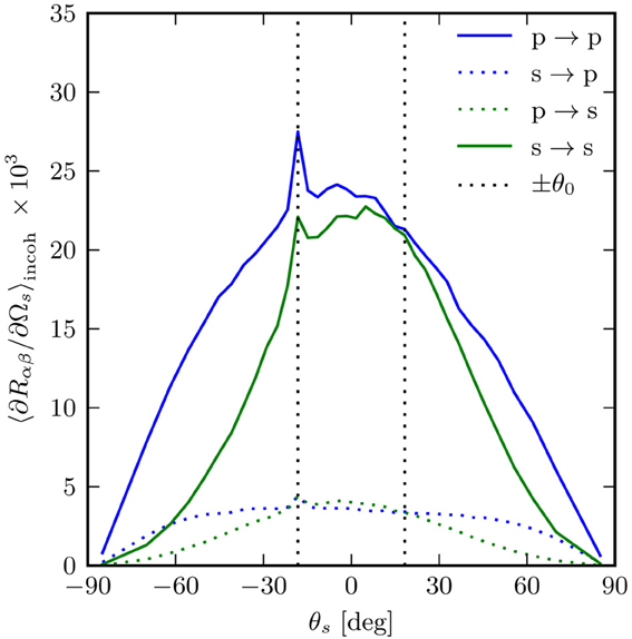
Figure 2. The incoherent component of the mean differential reflection coefficients (Equation 16) for the in-plane scattering from a rough silver surface as functions of scattering angle θ_s. The polar angle and wavelength (in vacuum) of the incident light were θ₀ = 18.2° and λ = 457.9nm, respectively, and the dielectric function of silver at this wavelength is ε₂(ω) = −7.5+0.24i. The surface power spectrum was Gaussian (Equation 3), with correlation lengths a₁ = a₂ = 0.25λ and the rms height was δ = 0.025λ. The surface covered an area L × L, where L = 25λ, and the surface was discretized on a grid of 319 × 319 points. The position of the specular peak (not present in the incoherent component) and the enhanced backscattering peak are indicated by the vertical dashed lines. A total of 14,200 surface realizations were used to calculate the mean DRCs.

FIGURE 3

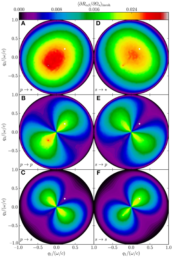
Figure 3. (A–F) Incoherent part of the mean differential reflection coefficient (Equation 16), showing the full angular distribution as a function of outgoing lateral wave vector. All parameters are the same as in Figure 2. The specular position is indicated by the white dots.

Figure 2 shows the in-plane scattering for this system. The enhanced backscattering peak, a multiple scattering phenomenon, is clearly visible, and is as expected strongest in p → p scattering, since p-polarized light has a stronger coupling to surface plasmon polaritons (Simonsen, 2010b). Figure 3 shows the full angular distribution of the mean DRC for the same system. In Figures 3A–C and D–F the incident light was p- and s-polarized, respectively. Figures 3C,F show scattering into s-polarization, Figures 3B,E show scattering into p-polarization and in Figures 3A,D the polarization of the scattered light was not recorded. In particular from Figure 3B, we observe that the enhancement features seen in Figure 2 at angular position θ_s = −θ₀, are indeed enhancements in a well-defined direction corresponding to that of retro-reflection, and not some intensity ridge structure about this direction [as has been seen for other scattering systems (Simonsen et al., 2010b)]. Moreover, the structures of the angular distribution of the intensity of the scattered light depicted in Figure 3 are consistent with what was found by recent studies by using other numerical methods (Simonsen et al., 2010a,b).

A test of energy conservation was performed by simulating the scattering of light from a non-absorbing silver surface [Im ε₂(ω) = 0] with otherwise the same parameters as those used to obtain the results of Figures 2, 3. For this scattering system we found | − 1| ≤ 0.0003, i.e., energy is conserved to within 0.03%, something that testifies to the accuracy of the approach and a satisfactory discretization.

As a further test, we studied the scattering from a set of (absorbing) silver surfaces with the same parameters used to obtain Figures 2, 3, except that the rms roughness δ was varied between 0 and 0.045λ, while the correlation lengths were held constant at a₁ = a₂ = 0.25λ ≡ a. For the purpose of comparison, we also performed simulations for a similar set of surfaces but assuming no absorption, i.e., we used ε₂(ω) = −7.5. The results of these tests are presented in Figure 4.

FIGURE 4

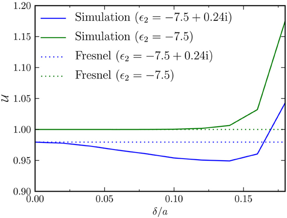
Figure 4. Ratio of reflected power to incident power, , as a function of ratio between rms roughness and correlation length, δ/a. Surface size and resolution were the same as for Figure 2, and the surface was randomly rough with a Gaussian power spectrum, correlation length was kept constant at a = a₁ = a₂ = 0.25λ, while the rms roughness δ was varied from 0.0 to 0.045λ. The Fresnel coefficients (horizontal dotted lines) have been included for comparison.

The RRE is only valid for surfaces of small slopes (Maradudin, 2007). We have found that at least for the parameters used in obtaining Figure 4, our code gives good results for an rms roughness to correlation-length ratio δ/a ≲ 0.12, as judged by energy conservation. For larger values of δ/a, the results look qualitatively much the same, but the ratio of reflected to incident power starts to become non-physical (increasing past 1), as seen in Figure 4. It is noted that decreasing the sampling interval Δq, with unchanged, did not change this conclusion in any significant way, indicating that the observed lack of energy conservation was not caused by poor resolution in discretizing the integral over q_‖.

The next set of calculations we performed was for a dielectric substrate characterized by ε₂ = 2.64. Otherwise, all roughness parameters were the same as for the silver surface used to produce Figures 2, 3. The mean differential reflection coefficient for light scattered incoherently by the rough dielectric surface is presented in Figure 5. By comparing these results to those presented in Figure 3, we notice that the dielectric reflects less than the silver (the figures show only the incoherent scattering, but the same holds for the coherent part), which is as expected. The ratio of reflected to incident power for these data was = 0.0467 for p-polarized light at an angle of incidence of θ₀ = 18.2°. Moreover, from Figure 5 we also notice the absence of the enhanced backscattering peak, which is also to be expected since this phenomenon (for a weakly rough surface) requires the excitation of surface guided modes (Simonsen, 2010b). Note that for a transparent substrate, it is not possible to verify the conservation of energy without also calculating the transmitted field. Therefore, energy conservation has not been tested for the dielectric substrate geometry.

FIGURE 5

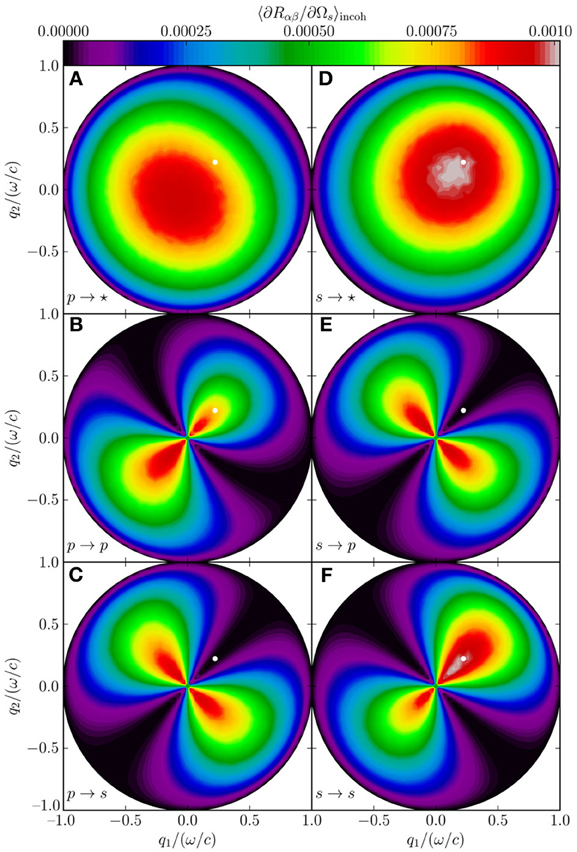
Figure 5. (A–F) The same as in Figure 3, except that ε₂ = 2.64, and the results are averaged over 21,800 randomly rough surfaces.

So far, we have exclusively considered surfaces with statistically isotropic roughness. For the results presented in Figure 6, we simulated the light scattering from a silver surface of the same parameters as those assumed in producing the results of Figures 2, 3, except that now the surface power spectrum was anisotropic, with correlation lengths a₁ = 0.25λ in the x₁ direction and a₂ = 0.75λ in the x₂ direction and an rms roughness of δ = 0.025λ. Figure 6 shows the incoherent part of the mean DRC averaged over 6800 surface realizations. In this case, there is more diffuse scattering along the x₁ direction than the x₂ direction, which is to be expected, since a shorter correlation length means the height of the surface changes more rapidly when moving along the surface in this direction. The interested reader is encouraged to consult Simonsen et al. (2011) for a more detailed study of light scattering from anisotropic surfaces.

FIGURE 6

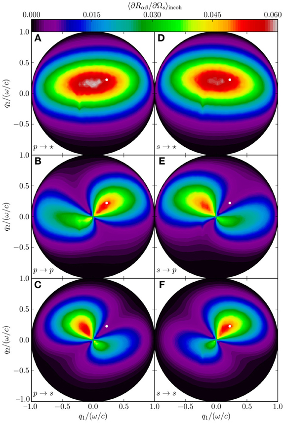
Figure 6. (A–F) The same as in Figure 3, except the correlation length of the Gaussian roughness, which is a₁ = 0.25λ in the x₁ direction and a₂ = 0.75λ in the x₂ direction, and the results are the average of an ensemble of 6800 surface realizations.

Finally, for the results presented in Figure 7, we have simulated the scattering of light from a surface of size 25λ × 25λ, discretized into 319 × 319 points, with ε₂(ω) = −16 + 1.088i, corresponding to silver at a wavelength λ = 632.8nm. The surface power spectrum was cylindrical (see Equation 4), with k₋ = 0.82ω/c, k₊ = 1.97ω/c and rms roughness δ = 0.025λ, and the angles of incidence were (θ₀, ϕ₀) = (1.6°, 45°). Figure 7 shows the in-plane, incoherent part of the mean differential reflection coefficient averaged over 7000 surface realizations.

FIGURE 7

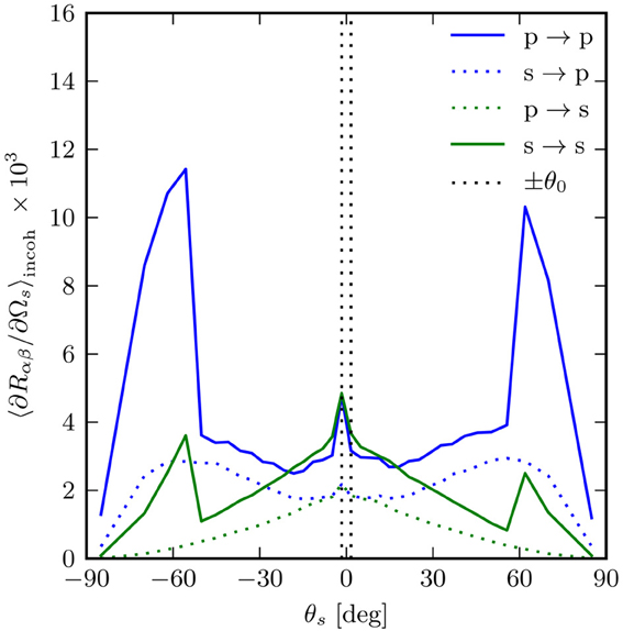
Figure 7. The incoherent component of the mean differential reflection coefficients (Equation 16) for the in-plane scattering from a rough silver surface as functions of scattering angle θ_s. The angles of incidence were θ₀ = 1.6° and ϕ₀ = 45°. The wavelength of the incident light was λ = 632.8nm for which the dielectric function of silver is ε₂(ω) = −16+1.088i. The surface power spectrum was of the cylindrical type (Equation 4), with k₋ = 0.82ω/c, k₊ = 1.97ω/c, and the rms roughness was δ = 0.025λ. A total of 7000 surface realizations were used to obtain the presented results.

From perturbation theory (Maradudin, 2007; Simonsen, 2010b), we know that for an incident wave of lateral wave vector k_‖ to be scattered via single scattering into a reflected wave of lateral wave vector q_‖, we must have g(q_‖ − k_‖) > 0, where g(k_‖) is the surface power spectrum (Equation 2). Since the power spectrum in this case is zero for |q_‖ − k_‖| < 0.82ω/c, we have no contribution from single scattering in the angular interval from θ_s = −53.5° to θ_s = 56.7° (for the angles of incidence assumed here). The enhanced backscattering peak, which is due to multiple scattering processes, is clearly visible in Figure 7 (at θ_s = −θ₀) partly because it is not masked by a strong single scattering contribution.

5.1. Comparison with Surface Integral Method

As a way to test our results, we have compared simulation data obtained by the method presented in this paper to results calculated by the surface integral method described by Simonsen et al. (2011). In both cases, we considered randomly rough silver surfaces at an incident wavelength of λ = 632.8nm, corresponding to a dielectric function of ε₂(ω) = −16 + 1.088i. The surface roughness was characterized by an isotropic Gaussian power spectrum, a correlation length of a = 0.25λ and rms roughness δ = 0.025λ. In the reduced Rayleigh simulations, we used a quadratic surface of edges L = 25λ, discretized to 319 × 319 points. In the surface integral simulations, the quadratic surface had edges L = 20λ, and was discretized on a grid of 160 × 160 points. Additionally, for the surface integral method an impedance boundary condition [see Simonsen et al. (2011) for details] and a finite size beam of full width 8 λ was used. The reason for the differences in parameters is the larger memory requirements of the surface integral method.

The results are presented in Figures 8 (p-polarized incident light) and 9 (s-polarized incident light), where the data from the reduced Rayleigh simulations are indicated by the solid lines, and the data for the surface integral method by the dashed lines. The results of Figures 8, 9 show that rather consistent results are obtained by the reduced Rayleigh method and the surface integral method at least for the scattering geometries studied here. Moreover, the total reflected energy obtained from the two methods were equal to three significant digits. However, we find that the surface integral method gives slightly less diffuse scattering than what is obtained by the reduced Rayleigh method. We speculate that this is caused by the more limited resolution used in the surface integral simulations.

FIGURE 8

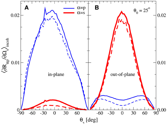
Figure 8. (A,B) Comparison of the incoherent component of the mean differential reflection coefficients for the in-plane and out-of-plane scattering of p-polarized waves from a rough silver surface. The results were obtained by two different numerical approaches: the solution of the reduced Rayleigh equation (solid lines), and by the use of the surface integral approach (Simonsen et al., 2011) (dashed lines). For the angle of incidence one assumed θ₀ = 25° and the wavelength of the incident light was λ = 632.8nm for which the dielectric function of silver is ε₂(ω) = −16 + 1.088i. The surface roughness was Gaussian, with a correlation length of a = 0.25λ and an rms roughness δ = 0.025λ. For the RRE simulations, a quadratic surface of edges L = 25λ, discretized to 319 × 319 points was used. In the surface integral simulations, the quadratic surface had edges L = 20λ, and 160 × 160 points.

FIGURE 9

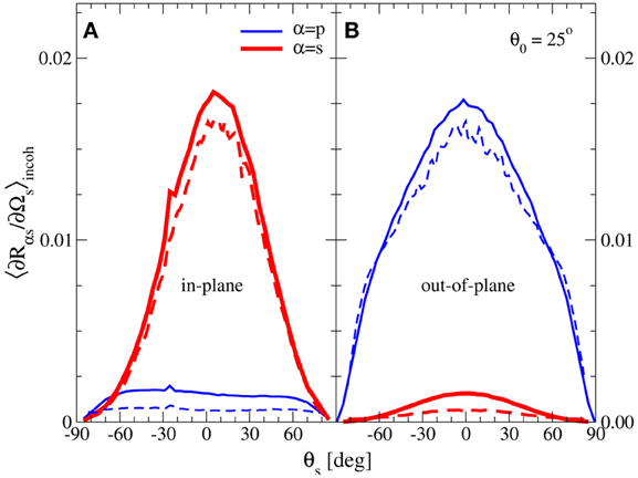
Figure 9. (A,B) The same as Figure 8, except the incident light was s polarized.

To increase the resolution in the surface integral simulations to a surface of 319 × 319 points would have required significantly more memory than the about 12 GB required to obtain the reduced Rayleigh simulation results presented here. Performing similar simulations by the surface integral method with an impedance boundary condition will require 308 GB of memory which is a 25 times increase compared to the requirements of the reduced Rayleigh method (Simonsen et al., 2011). Furthermore, if fully rigorous surface integral simulations should be performed, i.e., without imposing the impedance boundary conditions, the corresponding memory footprint of the simulations would be 1234 GB. These figures demonstrate some of the significant practical advantages that the RRE method has over the more general surface integral method.

5.2. Comparison to Experimental Data

As a further consistency check of our results, we have compared our simulation results to experimental scattering data from well characterized surfaces previously published by Navarrete Alcalá et al. (2009). The two surfaces in question were prepared on gold substrates. The first surface, referred to as sample 0061 by Navarrete Alcalá et al. (2009), had roughness characterized by a Gaussian power spectrum of correlation length a = 19μm and an rms roughness of δ = 0.5μm. The second surface, sample 7047, was characterized by Gaussian power spectrum with correlation length a = 9.5μm and an rms roughness of δ = 1.6μm. The wavelength of the incident light was λ = 10.6μm, for which the dielectric constant of gold is ε₂(ω) = −2489.77 + 2817.36i, and the polar angle of incidence was θ₀ = 30°.

In our simulations, we used the same roughness parameters as those used in the experiments by Navarrete Alcalá et al., and we considered quadratic surface realizations of edges L = 30λ, discretized to 319 × 319 points. However, in performing the simulations, we used an approximation where the substrate was treated as a perfect electric conductor. This approximation is expected to be valid as the skin depth of gold at the wavelength of the incident light is about 34nm (Navarrete Alcalá et al., 2009).

The advantage of assuming that the substrate is a perfect conductor is that the corresponding RREs will then not explicitly contain ε₂(ω) (Nordam et al., 2012a). If a large but finite value for ε₂(ω) is used, the series expansion used to calculate the integral I(γ|Q) (see Equations 14b and 20a) will be numerically unstable.

In Figures 10 (sample 0061) and 11 (sample 7047) we compare experimental scattering data to the corresponding simulation results obtained by the method just described. We observe from these figures generally good agreement for both polarizations of the incident light. The agreement between the measured and simulated data is best for s polarization. In the case of p polarization, there seems to be a slight shift of the simulated data compared to what was observed experimentally. It is speculated that this may be caused by a potential alignment problem in the experiment since the specular peak is not located at θ_s = θ₀ in the measurements corresponding to p polarization.

FIGURE 10

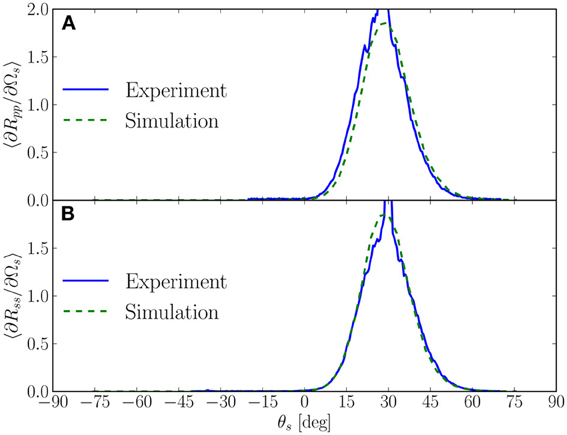
Figure 10. The mean differential reflection coefficient, showing in-plane scattering as function of the scattering angle θ_s. Experimental data obtained by Navarrete Alcalá et al. (2009) (sample 0061) for polar angle of incidence θ₀ = 30°, are shown by the blue solid lines, and our simulation results by the green dashed lines. The results shown are for (A) p to p scattering and, (B) s to s scattering. For the simulation results, only the incoherent component of the mean differential reflection coefficients are shown.

FIGURE 11

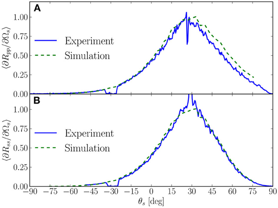
Figure 11. (A,B) The same as Figure 10, but now for sample 7047 from Navarrete Alcalá et al. (2009). It is noted that the slight shift of the simulations data relative the measured data for p to p scattering (A) is most likely caused by the angle of incidence used in the experiments being somewhat smaller than θ₀ = 30° which was assumed in the simulations.

6. Discussion

A challenge faced when performing a direct numerical solution of the RRE for the scattering of light from two-dimensional rough surfaces is the numerical complexity. In this section, we discuss some of these issues in detail.

6.1. Memory Requirements

Part of the challenge of a purely numerical solution of the RRE by the formalism introduced by this study, is that it requires a relatively large amount of memory. With approximately = (π/4)N²_q possible values for q_‖, the coefficient matrix of the linear equation system will contain approximately (2)² elements, where the factor 2 comes from the two outgoing polarizations. Hence, the memory required to hold the left hand side of the equation system will be approximately 4²η, where η is the number of bytes used to store one complex number.

If each element is a single precision complex number, which is what was used to obtain the results presented in this paper, then η = 8 bytes, and the matrix will require approximately 2π²N⁴_q bytes of memory for storage. For instance, with the choice N_x = 319, which was used in all the simulations presented in this paper, and that corresponds to N_q = 160 (Equation 23), the coefficient matrix will take up approximately 12 GB of memory.

Note that if we instead performed the q_‖ integration in Equation (14a) over a square domain of edge , the number of elements in the resulting coefficient matrix would be (2N²_q)² = (16/π²)(2)². Hence, by restricting the q_‖ integration present in the RRE to a circular domain of radius /2, the memory footprint of the simulation is approximately π²/16 ≈ 0.62 of what it would have been if a square integration domain of edge was used. For this reason, a circular integration domain has been used in obtaining the results presented in this paper. However, we have checked and found that using a square q_‖ integration domain of a similar size will not affect the results in any noticeable way. Indeed, if this was not the case, it would be a sign that was too small.

When determining the system size, we can freely choose the length of the edge of the square surface, L, and the number of sampling points along each direction, N_x. These parameters will then fix the resolution of the surface, Δx, the resolution in wave vector space, Δq, the number of resolved wave vectors, N_q, and the cutoff in the q_‖ integral, (see Equation 19, 24, 23, and 25). The combination of Δq and then determines the number of resolved wave vectors that actually fall inside the propagating region, |q_‖| < ω/c, which is identical to the number of data points used to produce, e.g., Figure 3.

As we are not free to choose all the parameters of the system, it is clear that some kind of compromise is necessary. The number of sampling points of the surface along each direction, N_x, and how it determines N_q via Equation (23), determines the amount of memory needed to hold the coefficient matrix, as well as the time required to solve the corresponding linear set of equations. Hence, the parameter N_x is likely limited by practical considerations, typically by available computer hardware or time. For a given value of N_x, it is possible to choose the edge of the square surface, L, to get good surface resolution, at the cost of poor resolution in wave vector space, or vice versa. Note also that changing L will change via Δq (see Equations 24 and 25). If is not large enough to include evanescent surface modes, like surface plasmon polaritons, multiple scattering will not be correctly included in the simulations, and the results can therefore not be trusted. The optimal compromise between values of N_x and L depends on the system under study.

6.2. Calculation Time

The simulations presented in this paper were performed on shared-memory machines with 24 GB of memory and two six-core 2.4 GHz AMD Opteron processors, running version 2.6.18 of the Linux operating system. The code was parallelized using the MPI library, and the setup of the linear set of equations ran on all 12 cores in the timing examples given. The linear equation solver used was a parallel, dense solver based on LU-decomposition (Press et al., 1992) (PCGESV from ScaLAPACK), which runs efficiently on all 12 cores. Setting up the equation system scaled almost perfectly to a large number of cores, while the solver scaled less well, due to the need for communication. Numerically solving the RRE for the scattering amplitudes associated with one realization of a rough surface, discretized onto a grid of 319 × 319 points, took approximately 17 min on the architecture described above, and required about 12 GB of memory. Out of this time, approximately 100 s was spent setting up the equation system, 950 s was spent solving it by LU decomposition, and typically around 1 s was spent on other tasks, including writing data to disk. Table 1 shows timing and memory details of the calculations, including other system sizes.

TABLE 1

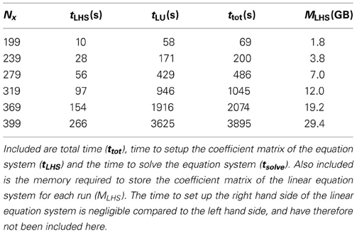
Table 1. Walltime spent to solve the RRE for various values of N_x on a shared-memory machine with two six-core 2.4 GHz AMD Opteron processors.

Based on the discussion in Section 6.1, we note that the use of a circular q_‖ integration domain also significantly reduces the time required to solve the resulting linear system of equations. When using a dense solver, the time to solve the systems scales as the cube of the number of unknowns. Thus we expect the CPU time to solve the matrix system for a circular integration domain of radius /2 to be about half (π³/2⁶) the time to solve the corresponding system using a square domain of edge .

The ratio of the time spent solving one equation system to the total simulation time per surface realization increases with increasing system size, as the time to set up the equation system is (N⁴_x), while the time to solve the linear system by LU decomposition scales as (N⁶_x). It is clear from Table 1 that for any surface of useful size the runtime is completely dominated by the time spent in solving the linear set of equations.

Since the time solving the equation system dominates the overall simulation time, we investigated if one could improve the performance of the simulations by using an iterative solver instead of a direct solver based on LU decomposition. For example, Simonsen et al. (2010b) recently reported good performance using BiCGStab (van der Vorst, 1992) on a dense matrix system of a similar size. In our preliminary investigations into using iterative solvers, we found that convergence with BiCGStab was slow and unreliable for our linear equation systems. However, it should be stressed that we did not use a preconditioning scheme, which could potentially yield significantly improved convergence. A detailed investigation of this issue is left for future work.

From Equation (14a) it follows that changing the angles of incidence and/or the polarization of the incident light changes only the right hand side of the equation system to be solved. Hence, an advantage of using LU decomposition (over iterative solvers) is that the additional time required to solve the system for several right hand sides is negligible, since the overall majority of time is spent factorizing the matrix. Conversely, the time spent using an iterative solver (like BiCGStab) will scale linearly with the number of right hand sides. For these reasons, we have chosen to use an LU-based solver.

6.3. GPU Implementation

Currently, performing simulations like those presented in this paper on a single desktop computer is prohibitively time consuming due to inadequate floating point performance. However, the increasing availability of powerful graphics processing units (GPUs) has the potential to provide computing power comparable to that of a powerful parallel machine, but at a fraction of the cost. As the most time-consuming step in our simulations is the LU decomposition of the system matrix (see Table 1), this is where efforts should be made to optimize the code. With this in mind, the simulation code was adapted to (optionally) employ version 1.0 of the MAGMA library (Agullo et al., 2011) for GPU-based LU decomposition. Performance was compared between a regular supercomputing service and a GPGPU (General Purpose GPU) testbed. On the regular service, the code was running on a single compute node containing two AMD 2.3 GHz 16-core processors and 32 GB of main memory. On the GPGPU testbed, the hardware consisted of a single Nvidia Fermi C2050 processor with 3 GB of dedicated memory and 32 GB of main system memory. For these two computer systems, the initial performance tests indicated that the LU decomposition took comparable time on the two architectures for a system of size N_q = 100 (the difference was less than 10%). The time using the GPGPU testbed included the transfer of the system matrix to and from the Fermi card and the decomposition of the matrix. Even though these results are preliminary, it demonstrates that there is a possibility of performing simulations like those reported in this study without having to resort to costly supercomputing resources. Instead, even with limited financial means, they may be performed on single desktop computers with a state-of-the-art GPU.

7. Conclusion

We have introduced a formalism for performing non-perturbative, purely numerical, solutions of the RRE for the reflection of light from two-dimensional penetrable rough surfaces, characterized by a complex dielectric function ε₂(ω). Implementation and performance issues of the proposed method, and various consistency checks of it, were presented and discussed.

As an example, we have used this formalism to carry out simulations of the scattering of p- or s-polarized light from two-dimensional randomly rough dielectric and metallic surfaces characterized by isotropic or anisotropic Gaussian and cylindrical power spectra. From the scattering amplitudes, obtained by solving the RRE, we calculate the mean differential reflection coefficients, and we calculate the full angular distribution of the scattered light, with polarization information. For the scattering of light from weakly rough metal surfaces, the mean differential reflection coefficient shows a well-defined peak in the retro-reflection direction (the enhanced backscattering phenomenon). From previous experimental and theoretical work, this is to be expected for such scattering systems. Moreover, the obtained angular distributions of the intensity of the scattered light show the symmetry properties found for strongly rough surfaces in recent studies using other simulation methods.

For the purpose of evaluating the accuracy of our simulation results, we used the conservation of energy for a corresponding non-absorbing scattering system. This is a required, but not sufficient, condition for the correctness of the numerical simulations. By this method, we found that within the validity of the RRE our code produces reliable results, at least for the parameters assumed in this study. In particular, for a rough non-absorbing metal surface of the parameters used in this study, energy was conserved to within 0.03%, or better. This testifies to the accuracy of the approach and a satisfactory discretization. Moreover, we also performed simulations of the scattered intensity for systems where the rms roughness of the surface was systematically increased from zero with the other parameters kept unchanged. It was found that energy conservation was well satisfied (for the parameters assumed) when the ratio of rms roughness (δ) to correlation length (a), satisfied δ/a ≲ 0.12.

We believe that the results of this paper provide an important addition to the collection of available methods for the numerical simulation of the scattering of light from rough surfaces. The developed approach can be applied to a wide range of scattering systems, including clean and multilayered scattering systems, that are relevant for numerous applications. The memory requirements, while not insignificant, are still smaller than for the surface integral method by about an order of magnitude. Hence, the current method can be applied to systems which were previously outside the reach of numerical simulations.

Conflict of Interest Statement

The authors declare that the research was conducted in the absence of any commercial or financial relationships that could be construed as a potential conflict of interest.

Acknowledgments

We would like to acknowledge the help of Dr. C. Johnson at the EPCC, University of Edinburgh, for help in parallelizing the code. We are also indebted to Dr. A. A. Maradudin for discussions on the topic of this paper, and Dr. E. Méendez and Dr. E. I. Chaikina, for making available the experimental data from Navarrete Alcalá et al. (2009). The work of Tor Nordam was mainly carried out with support from the Nordic Center of Excellence in Photovoltaics, funded by Nordic Energy Research (contract no. 06-Renew-C31). The work of Tor Nordam and Paul A. Letnes was partially carried out under the HPC-EUROPA2 project (project number: 228398) with support of the European Commission—Capacities Area—Research Infrastructures. The work also received support from NTNU by the allocation of computer time.

Footnotes

1. ^For the calculations used to generate the results presented in this paper, this would amount to evaluating I(γ|Q_‖) on the order of 10¹⁰ times.
2. ^Note that since the FFT always resolves the zero frequency, and the FFT of a purely real signal is symmetric about the zero frequency under complex conjugation, it is always possible to calculate an odd number of elements along each axis of the FFT

References

Agranovich, V. M., and Gartstein, Y. N. (2006). Spatial dispersion and negative refraction of light. Phys. Usp. 49, 1029–1944. doi: 10.1070/PU2006v049n10ABEH006067

CrossRef Full Text

Agullo, E., Augonnet, C., Dongarra, J., Faverge, M., Langou, J., Ltaief, H., et al. (2011). “LU factorization for accelerator-based systems,” in 2011 9th IEEE/ACS International Conference on Computer Systems and Applications (AICCSA) (Sharm El-Sheikh: IEEE), 217–224.

Bass, F. G., and Fuks, I. M. (1979). Wave Scattering from Statistically Rough Surfaces. Oxford: Pergamon.

Baumeier, B., Leskova, T. A., and Maradudin, A. A. (2009). Cloaking from surface plasmon polaritons by a circular array of point scatterers. Phys. Rev. Lett. 103:246803. doi: 10.1103/PhysRevLett.103.246803

Pubmed Abstract | Pubmed Full Text | CrossRef Full Text

Bonnet, M. (1999). Boundary Integral Equation Methods for Solids and Fluids. Chichester: Wiley.

Boyd, J. P. (2001). Chebychev and Fourier Spectral Methods. 2nd Edn. New York, NY: Dover.

Brown, G. C., Celli, V., Haller, M., and Marvin, A. (1984). Vector theory of light scattering from a rough surface: unitary and reciprocal expansions. Surf. Sci. 136, 381–397. doi: 10.1016/0039-6028(84)90619-8

CrossRef Full Text

Freilikher, V., Pustilnik, M., and Yurkevich, I. (1994). Wave scattering from a bounded medium with disorder. Phys. Lett. A 193, 467–470. doi: 10.1016/0375-9601(94)90541-X

CrossRef Full Text

Greffet, J.-J. (1988). Scattering of electromagnetic waves by rough dielectric surfaces. Phys. Rev. B 37, 6436–6441. doi: 10.1103/PhysRevB.37.6436

Pubmed Abstract | Pubmed Full Text | CrossRef Full Text

Gu, Z.-H., Dummer, R. S., Maradudin, A. A., McGurn, A. R., and Méendez, E. R. (1991). Enhanced transmission through rough-metal surfaces. Appl. Opt. 30, 4094–4102. doi: 10.1364/AO.30.004094

Pubmed Abstract | Pubmed Full Text | CrossRef Full Text

Hackbush, W. (1995). Integral Equations: Theory and Numerical Treatment. Basel: Birkhauser Verlag.

Harrington, R. F. (1993). Field Computation by Moment Methods. IEEE Press Series on Electromagnetic Wave Theory. New York, NY: Wiley-IEEE Press. doi: 10.1109/9780470544631

CrossRef Full Text

Jackson, J. D. (2007). Classical Electrodynamics. 3rd Edn. New York, NY: John Wiley and Sons.

Jin, J. (2002). The Finite Element Method in Electromagnetics. 2nd Edn. New York, NY: Wiley-IEEE Press.

Joannopoulos, J. D., Johnson, S. G., Winn, J. N., and Meade, R. D. (2008). Photonic Crystals: Molding the Flow of Light. 2nd Edn. Princeton, NJ: Princeton University Press.

Kampen, N. G. V. (2007). Stochastic Processes in Physics and Chemistry. 3rd Edn. Amsterdam: Elsevier.

Kern, A. M., and Martin, O. J. F. (2009). Surface integral formulation for 3d simulations of plasmonic and high permittivity nanostructures. J. Opt. Soc. Am. A 26, 732–740. doi: 10.1364/JOSAA.26.000732

Pubmed Abstract | Pubmed Full Text | CrossRef Full Text

Leskova, T. A. (2010). The reduced Rayleigh equation for reflection of light from two-dimensional randomly rough films deposited on flat substrates. Unpublished.

Madrazo, A., and Maradudin, A. A. (1997). Numerical solutions of the reduced Rayleigh equation for the scattering of electromagnetic waves from rough dielectric films on perfectly conducting substrates. Opt. Commun. 134, 251–263. doi: 10.1016/S0030-4018(96)00402-6

Pubmed Abstract | Pubmed Full Text | CrossRef Full Text

Mainguy, S., and Greffet, J.-J. (1998). A numerical evaluation of Rayleigh's theory applied to scattering by randomly rough dielectric surfaces. Waves Random Media 8, 79–101. doi: 10.1080/13616679809409831

CrossRef Full Text

Mandelstam, L. (1913). Über die rauhigkeit freier flüssigkeitsober-flächen. Ann. Phys. (Leipzig) 346, 609–624. doi: 10.1002/andp.19133460808

CrossRef Full Text

Maradudin, A. A. (ed.). (2007). Light Scattering and Nanoscale Surface Roughness. New York, NY: Springer-Verlag. doi: 10.1007/978-0-387-35659-4

CrossRef Full Text

Maradudin, A. A. (ed.). (2011). Structured Surfaces as Optical Metamaterials. New York, NY: Cambridge University Press. doi: 10.1017/CBO9780511921261

CrossRef Full Text

Maradudin, A. A. (2012). The reduced Rayleigh equation for transmission of light trough a two-dimensional randomly rough surface. Unpublished.

Maradudin, A. A., Méendez, E. R., and Leskova, T. A. (2008). Designer Surfaces. New York, NY: Elsevier Science.

Maradudin, A. A., Michel, T., McGurn, A. R., and Méndez, E. R. (1990). Enhanced backscattering of light from a random grating. Ann. Phys. (NY) 203, 255–307. doi: 10.1016/0003-4916(90)90172-K

Pubmed Abstract | Pubmed Full Text | CrossRef Full Text

McGurn, A. R., and Maradudin, A. A. (1996). Perturbation theory results for the diffuse scattering of light from two-dimensional randomly rough metal surfaces. Wave Random Media 6, 251–267. doi: 10.1088/0959-7174/6/3/006

CrossRef Full Text

McGurn, A. R., Maradudin, A. A., and Celli, V. (1985). Localization effects in the scattering of light from a randomly rough grating. Phys. Rev. B 31, 4866–4871. doi: 10.1103/PhysRevB.31.4866

Pubmed Abstract | Pubmed Full Text | CrossRef Full Text

Méendez, E., and O'Donnell, K. (1987). Observation of depolarization and backscattering enhancement in light scattering from Gaussian random surfaces. Opt. Commun. 61, 91–95. doi: 10.1016/0030-4018(87)90225-2

CrossRef Full Text

Méndez, E. R., García-Guerrero, E. E., Leskova, T. A., Maradudin, A. A., Muñoz-Lóopez, J., and Simonsen, I. (2002). Design of one-dimensional random surfaces with specified scattering properties. Appl. Phys. Lett. 81, 798–800. doi: 10.1063/1.1495900

Pubmed Abstract | Pubmed Full Text | CrossRef Full Text

Millar, R. F. (1969). On the Rayleigh assumption in scattering by a periodic surface. Math. Proc. Camb. 65, 773–791. doi: 10.1017/S0305004100003613

CrossRef Full Text

Millar, R. F. (1971). On the Rayleigh assumption in scattering by a periodic surface. II. Math. Proc. Camb. 69, 217–225. doi: 10.1017/S0305004100046570

CrossRef Full Text

Navarrete Alcalá, A. G., Chaikina, E. I., Méndez, E. R., Leskova, T. A., and Maradudin, A. A. (2009). Specular and diffuse scattering of light from two-dimensional randomly rough metal surfaces: experimental and theoretical results. Wave Random Media 19, 600–636. doi: 10.1080/17455030903033208

CrossRef Full Text

Nieto-Vesperinas, M. (2006). Scattering and Diffraction in Physical Optics. 2nd Edn. Singapore: World Scientific Publishing Company. doi: 10.1142/5833

CrossRef Full Text

Nordam, T., Letnes, P. A., Simonsen, I., and Maradudin, A. A. (2012a). Numerical solutions of the Rayleigh equations for the scattering of light from a two-dimensional randomly rough perfectly conducting surface. Unpublished.

Nordam, T., Letnes, P. A., Simonsen, I., and Maradudin, A. A. (2012b). Satellite peaks in the scattering of light from the two-dimensional randomly rough surface of a dielectric film on a planar metal surface. Opt. Exp. 20, 11336–11350. doi: 10.1364/OE.20.011336

Pubmed Abstract | Pubmed Full Text | CrossRef Full Text

Ogilvy, J. A. (1991). Theory of Wave Scattering from Random Rough Surfaces. Bristol: IOP Publishing.

Pendry, J. B., Martín-Moreno, L., and Garcia-Vidal, F. J. (2004). Mimicking surface plasmons with structured surfaces. Science 305, 847–848. doi: 10.1126/science.1098999

Pubmed Abstract | Pubmed Full Text | CrossRef Full Text

Pendry, J. B., Schurig, D., and Smith, D. R. (2006). Controlling electromagnetic fields. Science 312, 1780–1782. doi: 10.1126/science.1125907

Pubmed Abstract | Pubmed Full Text | CrossRef Full Text

Press, W. H., Teukolsky, S. A., Vetterling, W. T., and Flannery, B. P. (1992). Numerical Recipes in Fortran. The Art of Scientific Computing. 2nd Edn. Cambridge: Cambridge University Press.

Rayleigh, L. (1896). The Theory of Sound. 2nd Edn, Vol. 2. London: MacMillan, 89, 297–311.

Rayleigh, L. (1907). On the dynamical theory of gratings. Proc. R. Soc. Lon. Ser. A 79, 399–416. doi: 10.1098/rspa.1907.0051

CrossRef Full Text

Schurig, D., Mock, J. J., Justice, B. J., Cummer, S. A., Pendry, J. B., Starr, A. F., et al. (2006). Metamaterial electromagnetic cloak at microwave frequencies. Science 314, 977–980. doi: 10.1126/science.1133628

Pubmed Abstract | Pubmed Full Text | CrossRef Full Text

Simonsen, I. (2010a). Enhanced back and forward scattering in the reflection of light from weakly rough random metal surfaces. Phys. Status Solidi B 247, 2075–2083. doi: 10.1002/pssb.200983938

CrossRef Full Text

Simonsen, I. (2010b). Optics of surface disordered systems: a random walk through rough surface scattering phenomena. Eur. Phys. J. Spec. Top. 181, 1–103. doi: 10.1140/epjst/e2010-01221-4

CrossRef Full Text

Simonsen, I., Kryvi, J. B., Maradudin, A. A., and Leskova, T. A. (2011). Light scattering from anisotropic, randomly rough, perfectly conducting surfaces. Comp. Phys. Commun. 182, 1904–1908. doi: 10.1016/j.cpc.2011.01.010

CrossRef Full Text

Simonsen, I., and Maradudin, A. A. (1999). Numerical simulation of electromagnetic wave scattering from planar dielectric films deposited on rough perfectly conducting substrates. Opt. Commun. 162, 99–111. doi: 10.1016/S0030-4018(99)00036-X

CrossRef Full Text

Simonsen, I., Maradudin, A. A., and Leskova, T. A. (2010a). The scattering of electromagnetic waves from two-dimensional randomly rough penetrable surfaces. Phys. Rev. Lett. 104:223904. doi: 10.1103/PhysRevLett.104.223904

Pubmed Abstract | Pubmed Full Text | CrossRef Full Text

Simonsen, I., Maradudin, A. A., and Leskova, T. A. (2010b). Scattering of electromagnetic waves from two-dimensional randomly rough perfectly conducting surfaces: the full angular intensity distribution. Phys. Rev. A 81:013806. doi: 10.1103/PhysRevA.81.013806

Pubmed Abstract | Pubmed Full Text | CrossRef Full Text

Soubret, A., Berginc, G., and Bourrely, C. (2001a). Application of reduced Rayleigh equations to electromagnetic wave scattering by two-dimensional randomly rough surfaces. Phys. Rev. B 63:245411. doi: 10.1103/PhysRevB.63.245411

CrossRef Full Text

Soubret, A., Berginc, G., and Bourrely, C. (2001b). Backscattering enhancement of an electromagnetic wave scattered by two-dimensional rough layers. J. Opt. Soc. Am. A 18, 2778–2788. doi: 10.1364/JOSAA.18.002778

Pubmed Abstract | Pubmed Full Text | CrossRef Full Text

Stratton, J. A. (2007). Electromagnetic Theory. IEEE Press Series on Electromagnetic Wave Theory. New York, NY: Wiley-IEEE Press.

Taflove, A., and Hagness, S. C. (2005). Computational Electrodynamics: The Finite-Difference Time-Domain Method. 3rd Edn. Norwood, MA: Artech House.

Tishchenko, A. V. (2009). Numerical demonstration of the validity of the Rayleigh hypothesis. Opt. Exp. 17, 17102–17117. doi: 10.1364/OE.17.017102

Pubmed Abstract | Pubmed Full Text | CrossRef Full Text

van der Vorst, H. A. (1992). Bi-CGSTAB: a fast and smoothly converging variant of Bi-CG for the solution of nonsymmetric linear systems. SIAM J. Sci. Stat. Comp. 13, 631–644. doi: 10.1137/0913035

CrossRef Full Text

Volakis, J. L., Chatterjee, A., and Kempel, L. C. (2001). Finite Element Method Electromagnetics: Antennas, Microwave Circuits, and Scattering Applications. New York, NY: IEEE Press.

Voronovich, A. G. (1999). Wave Scattering from Rough Surfaces. 2nd Edn. Berlin: Springer Verlag. doi: 10.1007/978-3-642-59936-1

CrossRef Full Text

West, C. S., and O'Donnell, K. A. (1995). Observations of backscattering enhancement from polaritons on a rough metal surface. J. Opt. Soc. Am. A 12, 390–397. doi: 10.1364/JOSAA.12.000390

Pubmed Abstract | Pubmed Full Text | CrossRef Full Text

Zayats, A. V., Smolyaninov, I. I., and Maradudin, A. A. (2005). Nano-optics of surface plasmon polaritons. Phys. Rep. 408, 131–314. doi: 10.1016/j.physrep.2004.11.001

CrossRef Full Text