Fracture networks in sea ice

1. Introduction

Fracturing and refreezing of sea ice in the Kara Sea is a complex process, depending on temperature, wind, currents, freshwater influx from two large rivers, salinity and even the Coriolis force. The system has earlier been studied by Korsnes et al. [1], who found a scale-free area distribution of ice floes.

In this paper, we focus on the network of fractures in sea ice, how the fractures are created, and how they relate to each other. The aim of the present study is to acquire a general understanding of such fracturing.

Sea ice fracture networks are easily accessible, and the processes occur on a time scale which is good for studying the dynamics. Understanding sea–ice fracturing may help to understand other two-dimensional fracture systems. Fractures in sea ice are also an important factor in sea ice decrease during spring and summer, as ice that breaks up creates open areas which in turn absorbs more heat, speeding up the melting process [2]. The coverage of the ice cap is in turn a considerable factor in the Earths climate [3].

The Kara Sea is chosen for this study mainly for its complex dynamics in the coldest winter months, when areas are fractured and refrozen multiple times, so the fracturing process can be observed repeatedly. The degree of refreezing will depend on weather conditions and ice drift.

The presented data is based on the work done by Korsnes et al. [1], where synthetic aperture radar (SAR) images were used to find the size distribution of ice floes in an area in the Kara sea between January 1st, and March 29th 1994. At this time of year, sea ice covers the entire area.

During the last decade, modern network theory [4–6] has given important knowledge of how networks are structured, and how the structure emerges from network growth. Knowledge of social networks of individuals [7, 8], can be used to better understand how individuals interact. In the same way, the structure of the Internet on router level [9] is a product of how routers communicate, and properties of the connections between them. Metabolic networks shows how different metabolites react to each other [10], and together contribute to the complex behavior of cells.

In network theory, networks are represented by nodes and links, where the links may represent social, chemical, or physical interactions between the nodes. An important achievement of modern network theory has been within the understanding of how such networks grow from simple structures into complex networks, and how the growth process influences the final network [11].

The focus of the present work is to understand how a fracture in a severely fractured material relates to surrounding fractures. Fractures in homogeneous materials are well known [12], but when multiple fractures are already present, the material is no longer homogeneous. New fractures are in varying degree limited by existing fractures, meaning that the interaction between fractures become important.

In two-dimensional fracture networks, one may study the fracture network itself in the framework of modern network theory [13, 14]. However, this become problematic for three-dimensional fracture networks where the fractures are intersecting sheets. In order to describe fracture systems in the same way irrespectively of being two or three-dimensional, a different equivalent network must be constructed.

The dual network has exactly the properties that makes it possible to study two and three-dimensional fracture systems on the same footing. Let each fracture be a node and each intersection between fractures be a link between their respective nodes.

The dual network of fractures in rocks was studied in Andresen et al. [15]. Earlier, the dual network has been used to study the complexity of cities [16, 17]. These authors demonstrate that the complexity of a city is linked to the dual network constructed from its streets. They link the complexity to the number of times on the average a stranger will have to ask for directions to get from one point to another—and this number is associated to the number of intersections between streets one has to pass, which is the number of links on the dual lattice. Hence, complexity is directly linked to the standard distance measure on the dual network.

The complexity of a fracture network will influence its transport properties. This is in particular relevant for fractures in rock fractures in which transport of hydrocarbons, water and pollutants are important practical problems.

The present paper, however, focuses on the fracture–fracture interactions, and the object of our study is the network of fractures in sea ice on a geographical scale within the context of modern network theory.

Whereas other work has focused on the geometrical properties of fracture networks of sea ice, in particular in connection with fractal scaling properties [18] our study is concerned with topological properties. Hence, they complement each other.

The present work suggests a model based on the dual network view on fractures. The model is similar to the discrete fracture network (DFN) model presented by Darcel et al. [19], but it seems better to reproduce correlations between intersecting fractures, as investigated by Andresen et al. [15] for the DFN model. The model is based on the observation that fractures in sea ice often end when hitting existing fractures.

We find in the following differences between the sea ice networks considered here and the rock outcrop fractures studied by Andresen et al. [15]. The sea ice is on the scale of the length of the cracks, two-dimensional. The outcrop fractures represent on the other hand a two-dimensional cut through a set of three-dimensional sheetlike fractures in the rock. Hence, the two fracture systems are fundamentally different.

In the next section we describe the work flow from satellite images of fractured sea ice to the constructed dual lattice. In section 3, we analyze the topological data that ensue from the dual lattices constructed from the satellite images. Based on these data, we introduce a model for growth of fractures in ice which compares well with the data. We sum up our results in the last section.

2. From Fractures to Network

Our analysis is based on Synthetic Aperture Radar (SAR) images, as shown in Figure 1. The SAR images were taken by the ESA ERS-1 satellite in three-day intervals between January 1st and March 30th 1994. It is difficult to see leads on radar images, so to find the fracture network, Korsnes et al. [1] used an algorithm that recognizes areas of texture between two images, and finds areas which have been rigid in the time span between the images. Figure 1 shows how rigid areas are created from two successive SAR images. The rigid areas have common translation and rotation between the images, and are considered ice floes. From this we find the fractures by using a skeleton algorithm [20], and then decide which fractures continue through each intersection, by manually applying the decision rules listed below. In addition to the SAR images, we analyze two optical images taken over the East Siberian sea in early June 2000 and 2006, shown in Figure 2. It should be noted that the procedure we use for identifying the cracks limits us to only detecting active cracks.

FIGURE 1

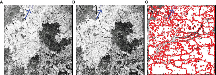
Figure 1. Panels (A,B) show two successive SAR radar images taken over the Kara sea on January 28th and 31st 1994. Panel (C) shows the identifies ice floes using the method described in Korsens et al. [1].

FIGURE 2

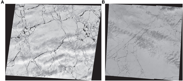
Figure 2. Optical images of fracture networks, taken over the East Siberian sea. (A) Date: June 7th 2000. (B) Date: June 5th 2006. Images courtesy of U.S.G.S [21].

2.1. Constructing the Dual Network

Figure 3 shows how the dual network is created, where each fracture is a node, and crossing or meeting fractures are linked together. The main challenge in this process is determining what is a fracture, in a large system, it is not always obvious which of the fractures that goes into an intersection that comes out on the other side. We use the following rules in the decision process:

1. If the intersection has three meeting leads, the most straight combination is typically the one that continues. The last one then stops.
2. If the intersection has more than three meeting leads, first look for the primary lead. That is the lead that came first, and which spans a larger part of the network than the rest. We identified the primary lead by having the same opening on both sides of the junction and not changing direction.
3. After the primary lead has been recognized, consider, by looking at direction, width, and the shape of the ice floes whether more of the leads continue.

FIGURE 3

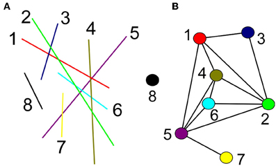
Figure 3. Example of creation of the dual network from a system of fractures. The fractures are followed through intersections, and define nodes in the dual network, nodes made by ridges that meet or cross each other get a link. (A) A small system of fractures and its dual network (B). The color and numbering of the node in (B) corresponds to the color and the numbering of the fracture in (A).

Figure 4 shows an example of how the dual network is created from SAR images.

FIGURE 4

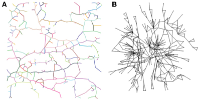
Figure 4. (A) Recognized fractures from Figure 1C. (B) Dual network of the system of fractures in (A), plotted with a force-directed algorithm [22] using the software tool Tulip 4.4.0. In the dual network, the fractures are interpreted as nodes, and links are made between intersecting fractures.

3. Analysis

3.1. Basic Network Properties

Clustering is a measure of connectivity on a local scale. The local clustering coefficient, C_i, is defined as the number of links between the nearest neighbors of a node, divided by the number of potential links between them. The clustering coefficient for the entire network, C, is the average of the local clustering coefficients [6]

$\begin{array}{cc}C=\frac{1}{N}{\displaystyle \sum _{i=1}^N{C}_i}=\frac{1}{N}{\displaystyle \sum _{i=1}^N\frac{2E_{nn,i}}{k_i(k_i-1)}},& \left(1\right)\end{array}$

where N is the total number of nodes in the network, k_i is the degree of node i, and E_nn is the number of links between the nearest neighbors of a node. The clustering coefficient can take values on the interval 0 ≤ C ≤ 1.

For comparison, we construct rewired and random networks, as explained below, with the same number of nodes and links as the found networks. In the local rewiring algorithm [23], links are rewired the following way: two links A → B and C → D are picked at random, and rewired to connect A → C and B → D. If the links A → C or B → D already exists, no changes are made, i.e., A → B and C → D are still connected. To create a rewired network, the local rewiring algorithm is run until network properties converge. During rewiring, the degree distribution stays unchanged. Random networks are made by placing the given number of links randomly between the given number of nodes.

Efficiency is a measure of global connectivity. The efficiency is defined by Boccaletti et al. [6]

$\begin{array}{cc}E=\frac{1}{N(N-1)}{\displaystyle \sum _{i,j\in N,i\ne j}\frac{1}{d_{ij}}},& \left(2\right)\end{array}$

where d_{i, j} is the minimal number of links used to traverse between nodes i and j.

In Table 1 values for clustering coefficients and efficiency for the different images are given. Table 2 shows average values for clustering coefficients and efficiency for networks created from SAR images, optical images, rock fractures [15] and the fracture network model explained later. The networks are characterized by a high clustering coefficient, and high efficiency. Both clustering and efficiency is higher than in the rock fracture networks investigated by Andresen et al. [15]. The high values found for both clustering and efficiency, gives the ridge networks properties of Small-World networks [24], where the characteristic distance between two nodes in the network is small compared to network size, while the network remains regular at a local level. Examples of Small-World networks range from social networks [7] to the Internet [9]. In Small-World networks, however, the characteristic path length scales at most as log(N), where N is the total number of nodes. Due to the small size of the investigated networks, this property is not checked here.

TABLE 1

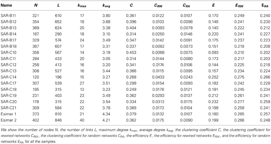
Table 1. Network properties for different samples of SAR and optical (Esimer) images.

TABLE 2

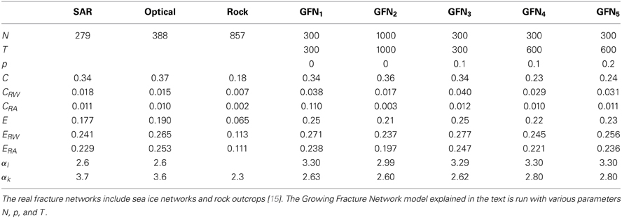
Table 2. Comparison of average network properties between fracture networks and models.

3.2. Scaling and Growth

The node degree distribution f(k), where the degree k is the number links from a node, is a central network property. The cumulative distribution function, F(k), is the probability that a node has degree lower than or equal to k. Figure 5 shows the cumulative degree distribution, as well as the cumulative distribution of fracture lengths, F(l). Both distributions are consistent with scale-freeness, with average slopes α_k and α_l shown in Table 2.

FIGURE 5

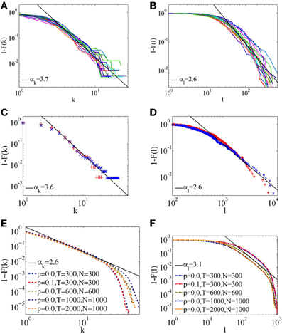
Figure 5. (A,C,E) Cumulative degree distribution for networks created from SAR images, optical images and GFN model respectively. (B,D,F) Cumulative length distribution for networks created from SAR images, optical images and GFN model, respectively.

To investigate the frequency of different degree–degree combinations, Maslov and Sneppen [23] introduced the correlation matrix

$\begin{array}{cc}C(k_1,k_2)=\frac{P(k_1,k_2)}{P_r(k_1,k_2)},& \left(3\right)\end{array}$

where P(k₁, k₂) is the probability that a node of degree k₁ is linked to a node of degree k₂. P_r(k₁, k₂) is the same for the average of rewired versions of the network. Each rewired network was made by a local rewiring algorithm [23] that ran until convergence of the clustering coefficient.

C(k₁, k₂) is symmetric, since the links in the dual network are undirected. To test the statistical significance of the correlation matrix Maslov and Sneppen [23] also introduced the significant correlation matrix

$\begin{array}{cc}Z(k_1,k_2)=\frac{P(k_1,k_2)-P_r(k_1,k_2)}{{\sigma }_r(k_1,k_2)},& \left(4\right)\end{array}$

where σ_r(k₁, k₂) is the standard deviation of P_r(k₁, k₂) for an ensemble of 1000 rewired networks. Z(k₁, k₂) can be both positive and negative. Z(k₁, k₂) ~ 0 indicates no significant correlation and |Z(k₁, k₂)| >> 0 indicates statistically robust results.

Figure 6 shows correlation and significant correlation profiles for networks created from SAR images, optical images, and from an instance of the fracture network model explained in the next section. The networks have strong correlations in the degree of neighboring nodes. That is, we see a strong tendency for nodes of high connectivity to connect to nodes of low connectivity and vice versa. Networks with this property are called disassortative. The strong correlations support the view that new fractures depend heavily on the existing network, and that the growth process is similar to that of the preferential growth mechanism [11].

FIGURE 6

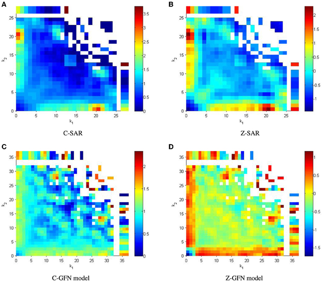
Figure 6. Correlation profiles C (k₁, k₂) and significant correlation profiles Z (k₁, k₂) showing. Results are smoothed. The white areas are degree–degree combinations that never were realized. (A,B) Average for the 16 SAR images from the Kara sea. (C,D) Average for 20 samples of the Growing Fracture Network model, with parameters N = 300 and p = 0.1, run for 1000 time steps. (A) C-SAR, (B) Z-SAR, (C) C-GFN model, (D) Z-GFN model.

Many real-world networks are created from a growth process that includes preferential growth [4, 11], in which new nodes are more likely to couple to existing nodes of high degree. Preferential growth leads to a scale-free degree distribution, and networks where a few major hubs maintain a high global efficiency.

In our case it is more natural to link preference for new nodes to the length of existing fractures, so that new fractures emerge from existing fractures with a probability proportional to the length of the existing fractures. In this model, the scale-free nature of the networks are not a consequence of preferential growth as in many other scale-free networks, but rather a consequence of geometrical properties.

If a square is split in four pieces, and then each piece is split again, indefinitely, the length distribution for the lines used to split the squares must be scale-free. This geometrical property is what gives the scale-free length distribution, not preferential growth itself.

Figure 7 shows fracture length as a function of degree for one of the investigated samples. All samples give similar results, showing that length and degree are strongly correlated, but that the points do not fall neatly on a line, as they would in a regular grid. This correlation is intuitively easy to understand by noting that longer cracks meet more cracks than shorter cracks. Hence, the corresponding node in the dual network has higher connectivity. Some areas of the fracture system are much more fractured than others, giving some long fractures with few intersections, and some short fractures with many intersections.

FIGURE 7

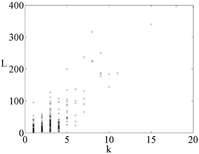
Figure 7. Fracture length l, plotted as a function of node degree, k, for a sample network made from a SAR image.

3.3. Growing Fracture Network Model

A proper analysis of the rheology of sea ice has been given by Girard et al. [25]. However, we propose here a fracture model that retains some of the qualitative features seen the competition between fracturing and refreezing of sea ice:

1. Start with one initial straight fracture spanning from one edge to the opposite edge. The direction of the initial fracture is arbitrary.
2. Choose one of the existing fractures with a probability proportional to the length of this fracture.
3. Pick a random point on the chosen fracture.
4. Choose an angle with which a new fracture will propagate from the existing fracture. This angle can be drawn from a distribution, to favor certain angles.
5. Propagate a new fracture in the found direction, and each time it hits an existing fracture, continue propagation with a probability p.
6. If the number of fractures is larger than a number N, remove a fracture. Which fracture to choose is inversely proportional to fracture length.
7. Iterate points 2–6.

Point 6 in the model, is intended as a very simple Poisson model for refreezing. It is very crude, as it does not allow for partial refreezing of leads, and should therefore only be taken as a process that messes up the fracture system. Figure 8 shows the fracture network model with p = 0.1, and N = 300 at six different time steps.

FIGURE 8

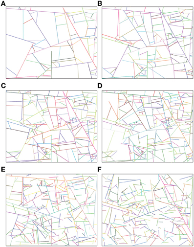
Figure 8. Images taken of the growing fracture network model at different times. For all images, the continuation parameter p is set to 0.1. (A) Image taken after 100 time steps. (B) Image taken after 200 time steps. (C) Image taken after 300 time steps, after 300 time steps, the refreezing process keeps the number of fractures at 300. (D) Image taken after 400 time steps. (E) Image taken after 1000 time steps. (F) Image taken after 3000 time steps.

A popular model for fractures is the discrete fracture network model (DFN) [19], which is based heavily on the fractal nature of fracture systems. In the DFN, the system is divided into smaller parts, where each part has a different density of fractures. The DFN captures the scale-free degree distribution of fractures, but the correlation profile is assortative [15], as opposed to the networks it aims to model. In an assortative network, nodes of similar connectivity tend to be connected to each other. The fracture network model proposed here, is intended to mimic the growth process of two-dimensional fracture networks, giving a much more correct correlation profile.

Some basic network properties of the model are listed in Table 2, showing that clustering and efficiency of the model are comparable to the sea–ice fracture networks. Both the length and degree distributions for the model are consistent with scale-freeness for the range of scales where edge effects are negligible, see Figure 5. The slope of the length distribution, α_l, is comparable to that of the sea–ice fracture networks, while the slope of the degree distribution, α_k, is considerably smaller than in the sea–ice fracture networks. By comparing images of the model (Figure 8) with the sea–ice images (Figure 2), we see that the model is considerably more homogeneous than the sea–ice networks, which may explain the difference in the degree distributions. For the model, α_l and α_k are much more similar than in the sea–ice networks, which supports this view, as in a completely homogeneous network, the two distributions would be equal. Figure 6 shows the degree–degree correlation profile of some sea–ice networks and an instance of the model, displaying the disassortative behavior of the model, which mimics the sea–ice networks very well. This behavior is the main feature of the model, which supports the correctness of the underlying mechanism.

4. Conclusions

We have studied how sea–ice fractures depend on each other by constructing the dual network where fractures are represented by nodes and intersections are links. The data are based on satellite images. We measure the different parameters that characterize the topology of networks.

Fractures in sea ice can propagate hundreds of kilometers if they remain uninterrupted, however, if a single existing fracture comes in the way, that may suffice to terminate the propagation. This basic observation illustrates the difference between fracturing in a homogeneous material, and fracturing in a fractured material. Thus the fractures interact very strongly, and early fractures more easily grow long.

The sea ice fracture network in the Kara Sea has been shown to have a scale-free distribution of fracture lengths. The dual network is also a scale-free network, with a scale-free degree distribution. The scale-free structure comes from a simple geometric relation, namely that as more fractures appear, there is less and less space for new fractures. This leads to a scale-free length distribution, and since the degree of a node is strongly correlated with fracture lengths, the degree distribution is also scale-free. The complex behavior of the ice, including refreezing and splitting of leads due to relative movements, tend to destroy the leads with many intersections, making the degree distribution steeper than one would otherwise expect.

Furthermore, the structure of the dual network is such that the degree–degree correlations are disassortative, meaning that nodes of a high degree tend to connect to nodes of low degree and vice versa. This structure supports the idea that long fractures are created early, while smaller fractures branch off from the longer ones at later stages. The branching ensures the network is connected, and that fractures relate strongly with each other. New fractures typically start and end at existing fractures. The growth results in a network with a high clustering coefficient, and high efficiency. The characteristic path length should, as a consequence of the growth process, grow as the logarithm of the number of fractures, classifying the network as a small-world network.

The Growing Fracture Network model differs from existing models [15, 19] mainly in the disassortative behavior of the correlation profile. Refreezing is included in the model as a Poisson refreezing process. The model reproduces fracture networks with realistic clustering, efficiency, and distribution of fracture lengths. It also reproduces the observed disassortative degree–degree correlation profiles. The degree distribution of the model, however, does not decay as quickly as in the present observed sea–ice fracture networks, indicating that the model creates overly homogeneous networks. It seems therefore not to capture all of the complexity in the Kara Sea system. This may, in part, be attributed to a crude model for refreezing.

Further investigation of the present fracture network model may contribute to better knowledge of formation of the networks.

Conflict of Interest Statement

The authors declare that the research was conducted in the absence of any commercial or financial relationships that could be construed as a potential conflict of interest.

Acknowledgments

Sigmund Mongstad Hope and Alex Hansen thank the Norwegian Research Council for funding through the ClIMIT program (grant no. 199970) and the RENERGI program (grant no. 217413/E20).

References

1. Korsnes R, Souza SR, Donangelo R, Hansen A, Paczuski M, Sneppen K. Scaling in fracture and refreezing of sea ice. Physica A. (2004) 331:291. doi: 10.1016/S0378-4371(03)00627-7

CrossRef Full Text

2. Andreas EL, Murphy B. Bulk transfer coefficients for heat and momentum over Leads and Polynyas. J Phys Oceanogr. (1986) 16:1875. doi: 10.1175/1520-0485(1986)016<1875:BTCFHA>2.0.CO;2

CrossRef Full Text

3. Clark PU, Alley RB, Pollard D. Northern hemisphere ice-sheet influences on global climate change. Science (1999) 286:1104. doi: 10.1126/science.286.5442.1104

CrossRef Full Text

4. Albert R, Barabási AL. Statistical mechanics of complex networks. Rev Mod Phys. (2002) 74:47. doi: 10.1103/RevModPhys.74.47

Pubmed Abstract | Pubmed Full Text | CrossRef Full Text

5. Newman MEJ. The structure and function of complex networks. SIAM Rev. (2003) 45:167. doi: 10.1137/S003614450342480

CrossRef Full Text

6. Boccaletti S, Latora V, Moreno Y, Chavez M, Hwang D-U. Complex networks: structure and dynamics. Phys Rep. (2006) 424:175. doi: 10.1016/j.physrep.2005.10.009

CrossRef Full Text

7. Milgram S. The small world problem. Psych Today (1967) 1:61.

8. Wasserman S, Faust K. Soc Netw Anal. Cambridge, MA: Cambridge University Press (1994). doi: 10.1017/CBO9780511815478

CrossRef Full Text

9. Yook S, Jeong H, Barabási A-L. Modeling the Internet's large-scale topology. Proc Natl Acad Sci USA. (2002) 99:13382. doi: 10.1073/pnas.172501399

Pubmed Abstract | Pubmed Full Text | CrossRef Full Text

10. Jeong H, Tombor B, Albert R, Oltvai ZN, Barabási A-L. The large-scale organization of metabolic networks. Nature (2000) 407:651. doi: 10.1038/35036627

Pubmed Abstract | Pubmed Full Text | CrossRef Full Text

11. Barabási A-L, Albert R. Emergence of scaling in random networks. Science (1999) 286:509. doi: 10.1126/science.286.5439.509

Pubmed Abstract | Pubmed Full Text | CrossRef Full Text

12. Thomson, RM. Physics of fracture. J Phys Chem Solids (1987) 48:965. doi: 10.1016/0022-3697(87)90114-4

CrossRef Full Text

13. Valentini L, Perugini D, Poli G. Physica A (2007) 377:323. doi: 10.1016/j.physa.2006.11.025

CrossRef Full Text

14. Valentini L, Perugini D, Poli G. The ‘small-world’ nature of fracture/conduit networks: possible implications for disequilibrium transport of magmas beneath mid-ocean ridges. J Volcanol Geotherm Res. (2007) 159:355. doi: 10.1016/j.jvolgeores.2006.08.002

CrossRef Full Text

15. Andresen CA, Le Goc R, Davy P, Hansen A, Hope SM. Topology of fracture networks. Front Phys. (2013) 1:7. doi: 10.3389/fphy.2013.00007

CrossRef Full Text

16. Rosvall M, Trusina A, Minnhagen P, Sneppen K. Networks and cities: an information perspective. Phys Rev Lett. (2005) 94:028701. doi: 10.1103/PhysRevLett.94.028701

Pubmed Abstract | Pubmed Full Text | CrossRef Full Text

17. Porta S, Crucitti P, Latora V. The network analysis of urban streets: a dual approach. Physica A (2006) 369:853. doi: 10.1016/j.physa.2005.12.063

CrossRef Full Text

18. Weiss J, Marsan, D. Scale properties of sea ice deformation and fracture. C R Acad Physique. (2004) 5:735–51. doi: 10.1016/j.crhy.2004.09.005

CrossRef Full Text

19. Darcel C, Bour O, Davy P, de Dreuzy JR. Connectivity properties of two-dimensional fracture networks with stochastic fractal correlation. Water Res. (2003) 39:1272. doi: 10.1029/2002WR001628

CrossRef Full Text

20. Van Dyne M, Tsatsoulis C. Extraction and analysis of sea ice leads from SAR images. In: Geoscience and Remote Sensing Symposium, 1993. IGARSS '93. Better Understanding of the Earth Environment; 1993 Aug 18–21; Tokyo (1993). p. 629–31.

21. U. S. Geological Survey. Global Fiducials Library, East Siberian Sea Preview Gallery (1999–2008). Available online at: http://gfl.usgs.gov/gallery/esiber_pub_gallery.shtml# (2010).

22. Frick A, Ludwig A, Mehldau, H. A fast adaptive layout algorithm for undirected graphs. In: Tamassia R, Tollis IG, editors. Graph Drawing. Springer Lecture Notes in Computer Science Vol. 894. Berlin: Springer (1995). p. 388.

23. Maslov S, Sneppen K. Specificity and stability in topology of protein networks. Science (2002) 296:910. doi: 10.1126/science.1065103

Pubmed Abstract | Pubmed Full Text | CrossRef Full Text

24. Watts DJ, Strogatz SH. Collective dynamics of ‘small-world’ networks. Nature (1998) 393:440. doi: 10.1038/30918

Pubmed Abstract | Pubmed Full Text | CrossRef Full Text

25. Girard L, Bouillon S, Weiss J, Amitrano D, Fichefet T, Legat V. A new modelling framework for sea ice mechanics based on elasto-brittle rheology. Ann Glaciol. (2011) 52:123–32. doi: 10.3189/172756411795931499

CrossRef Full Text