Moment-Preserving Theory of Vibrational Dynamics of Topologically Disordered Systems

1. Introduction

The vibrational properties of disordered solids at high frequencies, in the THz range, have been subject to great attention both from the experimental [2] and from the theoretical side [3] mainly because of the anomalies observed in the specific heat and in the thermal conductivity of glasses [4, 5]. The origin of an excess of the vibrational density of states (DOS) with respect to the Debye prediction in the THz region (an excess that is often referred to as “boson peak”) is thought to be the common origin of both anomalies. Also of interest, and at the origin of a lively debate [6–10], is the anomalous sound attenuation and the presence of a non-linear sound dispersion observed in the same frequency regime.

There is, nowadays, agreement on the fact that both the boson peak and the frequency dependence of the sound attenuation are the dynamical manifestation of the underlying topological (structural) disorder and that these features are not related to anharmonic interactions, to hopping processes or to other exotic phenomena like van-Hove singularities [11, 12]. The rich phenomenology observed in the dynamics of glasses in the THz frequency region can all be considered of harmonic origin [13, 14]. What is still missing is a deep understanding of the mechanisms that correlate the specificity of the topological disorder with the details of the observed dynamical anomalies.

In this respect, it becomes evident how important is the development of models of topological disorder with tunable properties.

The model approaches present in the literature for the influence of the disorder on the harmonic vibrational spectrum of solids can be grouped into models with waves in a spatially inhomogeneous media and mass-spring models. The wave approaches can again be grouped into a discription in terms of defect models [15–21] and fluctuating-elasticity approaches [9, 22–26].

In the defect models additional irregularities like atoms with heavy masses [15–17] or quasi-local harmonic oscillators [18–21], which couple to the Debye phonons, are introduced. The defect and coupling parameters are subject to a random distribution. In the fluctuating elasticity approach [9, 22–25, 27, 28] it is assumed that the elastic constants, (in particular the shear modulus) fluctuate around a mean value at different locations in space in a spatially correlated or uncorrelated fashion. Within this latter framework the disorder can be shown to lead to the anomalous increase of the DOS (and hence specific heat) with respect to the Debye prediction and to a contribution to the sound attenuation. It has been pointed out [27, 28] that in principle the defect description can be subsumed under the fluctuating-elasticity approach via a coarse-graining procedure.

In the disordered mass-spring models (which we shall address in the present contribution) one considers a set of mass points (mass M), which are fixed in space according to a given distribution and are connected by harmonic springs with spring constants K_ij. The equation of motion for the (scalar) displacements u_i from the rest positions is

$\begin{array}{ll}M\frac{d^2}{d{t}^2}{u}_i(t)=-{\displaystyle \sum _{j\ne i}}{K}_{ij}[u_i(t)-u_j(t)]& (1)\end{array}$

The disorder may be introduced by assuming a distribution of the K_ij on an otherwise ordered lattice (force-constant disorder) or placing the sites r_i randomly in space and then making the force constant depend on the site separations r_ij = |r_i − r_j|, i.e., K_ij = K(r_ij) (topological disorder).

There is an extended literature on such disordered mass-spring models [1, 29–42], which is due to the fact that they are considered to be relevant to the high-frequency vibrational dynamics of amorphous solids and liquids. They exhibit a wealth of anomalous phenomena including a boson peak [29, 32, 34–36, 38, 39, 41] and localization [33, 35, 42]. There is another point, which makes the investigation of models, which obey (Equation 1), interesting. If one replaces the double time derivative by a single one (and takes M = 1), one obtains the equation of motion of a random walker in a disordered system. The u_i(t) then take the meaning of the probability to find the walker at site i. It has been pointed out [1, 32, 43] that all anomalous features observed in the vibrational system (Equation 1) are also observed in the random-walk system: For example Rayleigh scattering in the vibrational system corresponds to an algebraic long-time tail in the velocity autocorrelation function in the random-walk system [1]. The boson peak corresponds to the onset of a strong frequency dependence of the conductivity in the random-walk system [32, 43].

The so-called Euclidean-Random-Matrix (ERM) approach introduced by Grigera et al. [39] is a systematic analytic approach to calculate the averaged vibrational spectrum and dynamical structure factor of systems govened by Equation (1). This is achieved by a high-frequency and high-density expansion, which is organized with the help of a diagram technique [1, 39, 40]

The ERM formalism allows for formulating self-consistent effective-medium approximations for the averaged Green's function corresponding to Equation (1). Such effective-medium approximations (“self-consistent ERM (SCERM) approximations,” which include the Rayleigh-scattering property¹ have been introduced by Ganter and Schirmacher [1].

In view of the fact that the ERM formalism enables to directly link the structure of a disordered solid to its vibrational spectrum it is desirable to establish a connection between this theory and the phenomenological heterogeneous elasticity theory. This, among others, will be done in the present paper. We start our investigation of the ERM mass-and spring model by showing that the self-consistent ERM approximations preserve the first two nontrivial moments (1st and 2nd) of the averaged level density. We then establish a link between the SCERM approximations and the self-consistent Born approximation (SCBA) of the heterogeneous elasticity theory. By means of this correspondence we devise a simplified SCERM theory (ERM-SCBA), which allows for solving the equations by a few iterations instead solving a set of integral equations.

In the second part of the paper we calculate numerically and in ERM-SCBA the level density and the first two nontrivial moments for a model with a Gaussian r dependence of the force constants. The moment calculations are done both for an infinite and a finite system. For the latter we find a strong N dependence of the moments, which is relevant for simulations in which only finite systems can be dealt with.

2. Formalism

2.1. Mass-Spring Model

We consider a mass-spring model with N mass points distributed at random in a volume V = L³ = N/ρ. We shall also consider the limit N → ∞ with fixed density ρ.

Equation (1) can be re-written as

$\begin{array}{ll}\frac{d^2}{d{t}^2}{u}_i=-{\displaystyle \sum _j}{D}_{ij}{u}_j& (2)\end{array}$

with the dynamical matrix D, having off-diagonal elements D_ij = −K(r_ij)/M and diagonal elements $D_{ii}=-\sum _{i\ne j}{D}_{ij}=\sum _{i\ne j}K(r_{ij})/M$. D has N eigenvalues ${\lambda }_p={\omega }_p^2$, where ω_p are the eigenfrequencies.

2.2. Density of States and Spectral Moments

The density of states g(ω) and the density of eigenvalues (“levels”) ρ(λ) are given by

$\begin{array}{l}\rho (\lambda )=\frac{1}{2}\omega g(\omega )=\frac{1}{N}\langle {\displaystyle \sum _p\delta }(\lambda -{\lambda }_p)\rangle \\ =\langle \frac{1}{N\pi }{I}m\{\text{tr}{[s𝟙+D]}^{-1}\}\rangle & (3)\end{array}$

where s = −ω² − iϵ, 𝟙 is the unit matrix and 〈… 〉 denotes a configurational average. Again λ = ω² denotes the eigenvalues of the dynamical matrix. Due to the sum rule $\sum _i{D}_{ij}=0$ (translation invariance) the dynamical matrix has always a “trivial” eigenvalue λ = 0 and, more important, there exists always an interval 0 < λ < λ*, in which a Debye law is valid, i.e., g(ω) ∝ ω² ↔ ρ(λ) ∝ λ^1/2.

In the present paper we thoughout assume a random distribution of points with density $P(r_1\dots r_i\dots r_N)=V^{-N}$. The n-th spectral moment of the level density is defined as

$\begin{array}{ll}{M}^{(n)}={\displaystyle \int }d\lambda {\lambda }^n\rho (\lambda ).& (4)\end{array}$

With the present definition of ρ(λ), the zeroth moment turns out to be equal to one, therefore the moments are automatically “normalized”. Let's also define the “central” moments:

$\begin{array}{ll}{M}_c^{(n)}={\displaystyle \int }d\lambda {(\lambda -\bar{\lambda })}^n\rho (\lambda )& (5)\end{array}$

with $\bar{\lambda }\doteq M^{(1)}$.

As stated above, the dynamical matrix has always the “trivial” eigenvalue, λ = 0. This has a non-negligible effect on the higher moments (specifically, it effects $M_c^{(n)}$). Therefore, we define a “non trivial” density of states, $\widehat{\rho }(\lambda )$, where the vanishing eigenvalue is excluded from the sum:

$\begin{array}{ll}\widehat{\rho }(\lambda )=\frac{1}{N-1}{\displaystyle \sum _{p|{\lambda }_p\ne 0}}\delta (\lambda -{\lambda }_p)& (6)\end{array}$

Let's call ${\widehat{M}}^{(n)}$ and ${\widehat{M}}_c^{(n)}$ the corresponding moments.

As far as the “hat” moments, we note that all the moments with n > 0 are unaffected (add or subtract ${\lambda }_p^n$, with λ_p = 0), but the normalization ((N − 1) instead of N) is different. The “hat” moments are thus obtained by multiplying the “non-hat” ones with N/(N − 1).

The moments M⁽ⁿ⁾ can be directly related to the dynamical matrix via:

$\begin{array}{ll}{M}^{(n)}={\displaystyle \int }d\lambda {\lambda }^n\rho (\lambda )=\frac{1}{N}\langle {\displaystyle \sum _p}{\lambda }_p^n\rangle =\frac{1}{N}\langle tr\{{\text{D}}^n\}\rangle & (7)\end{array}$

We represent the moments in terms of the dimensionless function f(r) defined as K(r_ij) = K₀f(r_ij/σ) = K₀f_ij, where σ is the characteristic decay length and their average

$\begin{array}{ll}\langle f^n\rangle =\frac{1}{N(N-1)}\langle {\displaystyle \sum _{i\ne j}{f}_{ij}^n}\rangle =\frac{1}{V}{\displaystyle {\int }_V{d}^3}rf{(r/\sigma )}^n& (8)\end{array}$

The results for the moments (see Appendix) are

$\begin{array}{ll}{M}^{(1)}=\frac{K_0}{M}(N-1)\langle f\rangle & (9)\end{array}$

$\begin{array}{cc}\begin{array}{l}{M}^{(2)}={\left(\frac{K_0}{M}\right)}^2\left[2N\langle f^2\rangle +N^2{\langle f\rangle }^2\right]\\ M_c^{(2)}={\left(\frac{K_0}{M}\right)}^{2}N\left[2\langle f^2\rangle -{\langle f\rangle }^2\right]\\ {\widehat{M}}^{(2)}={\left(\frac{K_0}{M}\right)}^2\left[2N\langle f^2\rangle +N^2{\langle f\rangle }^2\right]\\ {\widehat{M}}_c^{(2)}={\left(\frac{K_0}{M}\right)}^{2}2N\left[\langle f^2\rangle -{\langle f\rangle }^2\right]\end{array}& (10)\end{array}$

In the N → ∞ limit it is useful to define the dimensionless constants and $\Gamma =\frac{1}{\rho {\sigma }^3}$, $f_0=\int d^{3}rf(r)$, and $f_0^{(2)}=\int d^{3}rf{(r)}^2$, where the integral is over the entire space.

In this limit the ${\widehat{M}}^{(2)}$ moments become equal to the ones without hat and we have

$\begin{array}{lll}{M}_{\infty }^{(1)}& =& \frac{K_0{f}_0}{M\Gamma }\\ M_{\infty }^{(2)}& =& 2\frac{K_0{f}_0^{(2)}}{M\Gamma }+{\left[M_{\infty }^{(1)}\right]}^2\\ M_{c,\infty }^{(2)}& =& 2\frac{K_0{f}_0^{(2)}}{M\Gamma }& (11)\end{array}$

2.3. Euclidean Random Matrix (ERM) Formalism

To make contact to the ERM formalism [1, 39, 40] we consider the Fourier transformed force constants

$\begin{array}{ll}t(q)\doteq \frac{\rho }{M}\tilde{K}(q)=\frac{K_0{f}_0}{M\Gamma }\tilde{f}(\sigma q)=t_0\tilde{f}(\sigma q)& (12)\end{array}$

with

$\begin{array}{ll}\tilde{f}(k)=\tilde{f}(k)=\frac{1}{f_0}{\displaystyle \int }{d}^{3}r{e}^{i\text{kr}}f(r)& (13)\end{array}$

so that $\tilde{f}(k=0)=1$ and $t_0=t(k=0)=M_{\infty }^{(1)}$.

The quantity of interest is the q dependent averaged Green's function

$\begin{array}{l}G(\text{q},s)=\langle \frac{1}{N}{\displaystyle \sum _{\ell m}}{e}^{i\text{q}(r_{\ell }-r_m)}{\left[s𝟙+\text{D}\right]}_{\ell m}^{-1}\rangle \\ =\frac{1}{s+t_0-t(q)-\Sigma (\text{q},s)}& (14)\end{array}$

where Σ(q, s) is the self-energy function and, as before, s = −λ − ϵ = −ω² − ϵ. The level density is obtained from the Green's function via

$\begin{array}{ll}\rho (\lambda )=\frac{1}{\pi }Im\{G_{\infty }(s)\}& (15)\end{array}$

with $G_{\infty }(s)={\displaystyle \underset{\left|\text{q}\right|\to \infty }{lim}}G(\text{q},s)$.

The self energy can (and has been [1, 39, 40]) calculated with increasing powers of the inverse density ρ. The lowest-order result is Σ⁽⁰⁾(q, s) = 0, so that in the high-density limit

$\begin{array}{ll}{G}^{(0)}(q,s)=\frac{1}{s+t_0-t(k)}& (16)\end{array}$

One can make contact between this high-density limit and the traditional liquid-phonon theory of Hubbard and Beeby [44] by identifying the “liquid dispersion” with $\Omega =\sqrt{t_0-t(k)}$ and the Einstein frequency with ${\Omega }_E=\sqrt{t_0}$.

The lowest-order nontrivial contribution to the self energy is [1, 39, 40]

$\begin{array}{ll}{\Sigma }^{(1)}(\text{q},s)={\displaystyle \sum _{\text{p}}}[t(\text{p}-\text{q})-t(\text{p}){]}^2{G}^{(0)}(\text{p},s)& (17)\end{array}$

Here ${\sum }_{\text{p}}$ denotes $\frac{1}{\rho {(2\pi )}^3}\int d^3\text{p}$.

It has been suggested [39, 40] that one might obtain a suitable self-consistent (i.e., non-perturbative) approximation by replacing G₀(p, s) in Equation (17) by the full Green's function G(p, s). However, as shown by Ganter and Schirmacher [1], this self-consistent scheme violates the requirement that the sound attenuation coefficient $\Gamma (\omega )\propto \underset{\left|\text{q}\right|\to 0}{\lim }\omega Im\{\Sigma (\text{q},s)\}/q^2$ should vary ∝ω⁴ (Rayleigh scattering). A self-consistent scheme, which preserves this property has been proposed [1] by introducing auxiliary quantities g(q, s) and σ(q, s).

Within the self-consistent ERM (SCERM) approximation the self energy is given by

$\begin{array}{ll}\Sigma (\text{q},s)={\displaystyle \sum _{\text{p}}}[t(\text{q}-\text{p})-t(p){]}^{2}g(p,s)& (18)\end{array}$

This relation between Σ(q, s) and the auxiliary quantities g(q, s) and σ(q, s) has been called “cactus-1-approximation” in Ganter and Schirmacher [1]. A more complicated relation (“cactus-2”) suggested also by Ganter and Schirmacher [1] shall not be considered here.

The auxiliary quantities σ(q, s) and g(q, s) obey the self-consistent set of equations

$\begin{array}{ll}g(q,s)=[s+t_0-t(q)-\sigma (q,s){]}^{-1}& (19)\end{array}$

$\begin{array}{l}\sigma (q,s)={\displaystyle \sum _p\left[t(q-\text{}p)-t(p)\right]}\left[t(q\text{}-\text{}p)-t(q)\right]g(p,s)\end{array}$

2.3.1. The Spectral Moments in the ERM Formalism

In order to relate the SCERM scheme outlined in the previous paragraph to the spectral moments, we perform a high frequency expansion of the Green's function. We take advantage of the Hilbert-Stieltjes transformation relating G(q, s) to its imaginary part:

$\begin{array}{ll}G(\text{q},s)=\frac{1}{\pi }{\displaystyle \int }\frac{G^{″}(\text{q},\lambda )}{s-\lambda }d\lambda & (20)\end{array}$

Performing the |q| → ∞ limit as prescribed in Equation (15), we obtain

$\begin{array}{l}{G}_{\infty }(s)={\displaystyle \int }\frac{\rho \left(\lambda \right)}{s-\lambda }d\lambda \\ =\frac{1}{s}{\displaystyle \sum _{n=0}^{\infty }}{\left(-\right)}^n{\displaystyle \int }(\frac{\lambda }{s}{)}^n\rho (\lambda )d\lambda \\ =\frac{1}{s}{M}^{(0)}-\frac{1}{s^2}{M}^{(1)}+\frac{1}{s^3}{M}^{(2)}-\dots & (21)\end{array}$

In the |q| → ∞ limit the Green's function of Equation (14) becomes (taking into account ${\displaystyle \underset{\left|\text{q}\right|\to \infty }{lim}}t(k)\to 0$)

$\begin{array}{l}{G}_{\infty }(s)=[s+t_0-{\Sigma }_{\infty }(s){]}^{-1}\\ =\frac{1}{s}-\frac{1}{s^2}[t_0-{\Sigma }_{\infty }(s)]+\frac{1}{s^3}[t_0-{\Sigma }_{\infty }(s){]}^2-\dots & (22)\end{array}$

In order to expand the self energy it is advisable to reformulate Equation (19), using the identy,

$\begin{array}{ll}{\displaystyle \sum _{\text{p}}}{h}_1(\text{q}-\text{p})h_2(\text{p})=-{\displaystyle \sum _{\text{p}}}{h}_2(\text{q}-\text{p})h_1(\text{p})& (23)\end{array}$

as

$\begin{array}{ll}\Sigma (\text{q},s)={\displaystyle \sum _{\text{p}}}[t(p)-t(\text{q}-\text{p})]t(p)[g(p,s)+g(\text{q}-\text{p},s)]& (24)\end{array}$

The |q| → ∞ limit is then

$\begin{array}{ll}{\Sigma }_{\infty }(s)={\displaystyle \sum _{\text{p}}}{t}^2(p)[g(p,s)+g_{\infty }(s)]& (25)\end{array}$

We are interested in the first two nontrivial moments, therefore we need the expansion in 1/s up to the cubic, 1/s³, term. By inspecting Equation (22), we note that it is sufficient to expand Σ_∞(s) up to 1/s to have G_∞(s) correct up to 1/s³. In Equation (25) the leading contribution is given by the high-frequency limit g(p, s) → 1/s. The leading result for Σ_∞(s) is then

$\begin{array}{ll}{\Sigma }_{\infty }(s)=\frac{2}{s}{\displaystyle \sum _{\text{p}}}{t}^2(p)+O(\frac{1}{s^2})& (26)\end{array}$

Inserting this equation into Equation (22):

$\begin{array}{ll}{G}_{\infty }(s)=\frac{1}{s}-\frac{1}{s^2}{t}_o+\frac{1}{s^3}\left[t_o^2+2{\displaystyle \sum _p{t}^2(p)}\right]-\dots & (27)\end{array}$

By comparing this equation with Equation (21) we have:

$\begin{array}{l}{M}^{(0)}=1\hfill \\ M^{(1)}=t_0\hfill \\ M^{(2)}=t_0^2+2{\displaystyle \sum _p{t}^2(p)}=t_0^2[1+2{\displaystyle \sum _p{\tilde{f}}^2(\sigma p)}]\hfill & (28)\end{array}$

Using the Parseval theorem one can easily show

$\begin{array}{ll}{\displaystyle \sum _p{t}^2(p)}=\frac{K_0{f}_0^{(2)}}{M\Gamma }=\frac{1}{2}{M}_{c,\infty }^{(2)}& (29)\end{array}$

so that the results Equations (11) and (28) are the same.

This means that the SCERM approximation not only preserves the Rayleigh scattering property, as emphasized in Ganter and Schirmacher [1] but also preserves the first three spectral moments. Because we used only the property ${\displaystyle \underset{\left|s\right|\to \infty }{lim}}g(\text{q},s)=1/s$, any theory for calculating the “internal” Green's function will have this property. The nontrivial task is to come up with such a theory. In the next but one paragraph we show that one can establish a link between the self-consistent ERM approximations [1] and the self-consistent Born approximation of the heterogeneous elasticity theory [9, 22–25]. By this correspondence we shall find a simplified theory for calculating the DOS.

2.3.2. The DOS in the SCERM Formalism

For calculating the level density we need the large-wavenumber limit of the self energy Σ_∞(s), Equation (25). In these expressions appears the large-wavenumber limit of the auxiliary quantities ${\sigma }_{\infty }={\displaystyle \underset{q\to \infty }{lim}}\sigma (q,s)$ and $g_{\infty }={\displaystyle \underset{q\to \infty }{lim}}g(q,s)$. In order to calculate these quantities we take the large wavenumber limit in the self-consistent equations (Equation 19) applying again the convolution identity (Equation 23) to obtain

$\begin{array}{ll}{\sigma }_{\infty }={\displaystyle \sum _p}t{(p)}^2{g}_{\infty }& (30)\end{array}$

$\begin{array}{ll}{g}_{\infty }=\frac{1}{s+t_0-{\sigma }_{\infty }}=\frac{1}{s+t_0-{\displaystyle {\sum }_{p}t{(p)}^2{g}_{\infty }}}& (31)\end{array}$

Equations (30) and (31) lead to a quadratic equation for g_∞ with the solution (“Hubbard Green's function” [15])

$\begin{array}{ll}{g}_{\infty }(s)\doteq g_{HE}(s)=\frac{2}{s+t_0+\sqrt{{\left[s+t_0\right]}^2-4{\displaystyle {\sum }_p}t{(p)}^2}}& (32)\end{array}$

Its imaginary part is a half-ellipse (HE), centered around t₀ with half width $2\sqrt{\sum _p{t}^2(p)}=\sqrt{2M_{c,\infty }^{(2)}}$.

Combining now Equations (25) and (30) we have

$\begin{array}{ll}{\Sigma }_{\infty }(s)={\Sigma }_{\infty }^{(1)}(s)+{\sigma }_{\infty }(s)& (33)\end{array}$

with

$\begin{array}{ll}{\Sigma }_{\infty }^{(1)}(s)={\displaystyle \sum _p}t{(p)}^{2}g(p,s)& (34)\end{array}$

Combining this with the expression (Equation 22) for G_∞(s) we get

$\begin{array}{ll}{G}_{\infty }\left(s\right)=g_{\infty }(s-{\Sigma }_{\infty }^{(1)}\left(s\right))=g_{HE}(s-{\Sigma }_{\infty }^{(1)}(s))& (35)\end{array}$

For the level density we then obtain

$\begin{array}{ll}\rho (\lambda )=\frac{1}{\pi }{I}m\left\{g_{HE}\left(s-{\Sigma }_{\infty }^{(1)}(s)\right)\right\}& (36)\end{array}$

with g_HE(s) given by Equation (32) and ${\Sigma }_{\infty }^{(1)}(s)$ according to Equation (34).

2.3.3. Relation to Heterogeneous-Elasticity Theory and New Self-Consistent ERM Theory

If we consider the self-consistency Equation (19) we realize that the main contributions to the integrals over wavevectors are restricted to |q| < 1/σ. This means that one does not make a big error, if one makes an expansion with respect to the parameter |q|σ, i.e., a hydrodynamic expansion. For t(q) we can write

$\begin{array}{ll}t(q)=t_0-q^2{c}_0^2& (37)\end{array}$

where

$\begin{array}{ll}{c}_0^2=-\frac{1}{2}\frac{{\partial }^2}{\partial q^2}t(q){|}_{q=0}& (38)\end{array}$

is the unrenormalized sound velocity. We now define a hydrodynamic self energy

$\begin{array}{ll}{\sigma }_1(s)={\displaystyle \underset{q\to 0}{lim}}\frac{1}{q^2}\sigma (q,s)& (39)\end{array}$

so that the auxiliary Green's function becomes

$\begin{array}{ll}g(\text{q},s)=\frac{1}{s+q^2(c_0^2-{\sigma }_1(s))}& (40)\end{array}$

In order to perform the limit of Equation (39) we use the Taylor Formula

$\begin{array}{l}t(q-p)-t(p)=t^{\prime }(p)\frac{qp}{p}\\ +\frac{1}{2}[t\prime \prime (p)p-t\prime (p)]\frac{{(qp)}^2}{p^3}+\frac{1}{2}t\prime (p)\frac{k^2}{p}& (41)\end{array}$

where t′(q) and t″(q) are the derivatives with respect to q = |q|. Realizing that only even powers of qp contribute to the p integral in Equation (19) we obtain the following self-consistent equation for σ(q, s)

$\begin{array}{ll}\sigma (q,s)=\frac{1}{q}{t}^{\prime }(q){\displaystyle \sum _p\frac{1}{p}}{t}^{\prime }(p)\left[{(\text{qp})}^2+\frac{1}{4}{q}^2{p}^2\right]g(\text{q},s)& (42)\end{array}$

Taking into account the angle average $\langle {(\text{q}\text{p})}^2\rangle =\frac{1}{3}{q}^2{p}^2$ and replacing t′(q)/q by its low-q limit $-2c_0^2$ we get

$\begin{array}{ll}{\sigma }_1(s)=\frac{7}{6}{c}_0^2{\displaystyle \sum _p}{p}^2[-t^{\prime }(p)/p]g(p,s)& (43)\end{array}$

Introducing the dimensionless wavenumber $\tilde{p}=\sigma p$ and the dimensionles self energy ${\tilde{\sigma }}_1(s)={\sigma }_1(s)/c_0^2$ we obtain

$\begin{array}{ll}{\tilde{\sigma }}_1(s)=\gamma \frac{1}{I_0}{\displaystyle {\int }_0^{\infty }d}\tilde{p}{\tilde{p}}^4\left[\text{}-\text{}{\tilde{f}}^{\prime }(\tilde{p})/\tilde{p}\right]\frac{1}{s{\sigma }^2/c_0^2+{\tilde{p}}^2\left[1-{\tilde{\sigma }}_1(s)\right]}& (44)\end{array}$

with the disorder parameter

$\begin{array}{ll}\gamma =\frac{7}{6{\pi }^2}{I}_0\frac{t_0{\sigma }^2}{c_0^2}\Gamma & (45)\end{array}$

and the normalization constant

$\begin{array}{ll}{I}_0={\displaystyle {\int }_0^{\infty }}d\tilde{p}{\tilde{p}}^2[-{\tilde{f}}^{\prime }(\tilde{p})/\tilde{p}]& (46)\end{array}$

We mention that the prefactors of Γ in Equation (45) are model dependent constants, which do not depend on any physical parameter. For the Gaussian force constants $t_0{\sigma }^2/c_0^2=2$ and $I_0=\sqrt{\pi }/2$.

Equation (45) is mathematical identical with the version of the SCBA for correlated fluctuating elastic constants [24, 25]. One has to make the replacements C(q) ↔ [−f′(q)/q], where C(q) is the Fourier-transformed correlation function of the elastic moduli, divided by their variance. The disorder parameter γ ∝ Γ = 1/ρσ³ is proportional to the relative variation of the fluctuating elastic modulus of a mass-spring model, evaluated by a coarse-graining procedure, as shown by Ganter and Schirmacher [1]. Because both for a Gaussian as for an exponential $\tilde{f}(\tilde{p})$ the integral in Equation (44) can be done analytically, the solution of this equation is a matter of a few iterations and is much easier and quicker than solving the integral Equation (19).

Taking these considerations into account we now propose the following simplified SCERM scheme, which we call ERM-SCBA: In this approximation we use in formula (Equation 34) for ${\Sigma }_{\infty }^{(1)}(s)$ the hydrodynamic g(q, s) of Equation (40) i.e.,

$\begin{array}{ll}{\Sigma }^{(1)}(s)={\displaystyle \sum _p}t{(p)}^2\frac{1}{s+q^2{(c}_0^2-{\sigma }_1(s))}& (47)\end{array}$

with the SCBA self energy σ₁(s) given by the SCBA Equation (43)

$\begin{array}{ll}{\sigma }_1(s)=\frac{7}{6}{c}_0^2{\displaystyle \sum _p}{p}^2[-t^{\prime }(p)/p]\frac{1}{s+q^2(c_0^2-{\sigma }_1(s))}& (48)\end{array}$

This new self-consistent scheme for calculating approximately the spectrum of a disordered mass-spring model is the most important result of the present paper.

We emphasize that this approximation still meets the requirements of

(i) Preserving the lowest two nontrivial moments,

(ii) Giving a Debye DOS for λ < λ*,

(iii) Leading to Rayleigh scattering in the same frequency range.

We shall investigate the accuracy of this approximation in the next chapter.

3. The Gaussian Force Constants

In this section we report the results for the case of the Gaussian shape for the force constants $K(r)=K_0{e}^{-\frac{1}{2}{(r/\sigma )}^2}$, so that we have f(r) = e^−r2/2, $f_0={(2\pi )}^{3/2}$ and $f_0^{(2)}={\pi }^{3/2}$. For the “vertex function” in Equation (44) we have

$\begin{array}{ll}-\frac{1}{\tilde{q}}\widetilde{f^{\prime }}(\tilde{q})=\tilde{f}(\tilde{q}).& (49)\end{array}$

3.1. Numerical Simulation

In order to compare the analytical expression for the spectral moments summarized in the next paragraph, and, more important, to test the level of accuracy of the different theoretical approximation for the DOS spectral shape, we run a numerical simulation of the dynamics in the specific case of Gaussian shape for K(r_ij). For different values of the couple of parameters (N, Γ) we randomly chose N points (${\bar{r}}_i$) distributed in a box of size L = 1, set up the dynamical matrix with K₀=1 and M = 1, diagonalized this matrix using the Jacobi diagonalization algorithm [45], and set up the DOS as histogram of the obtained eigenvalues by repeating ≈1,000 times the random points choosing. The so obtained spectra are compared (see later) with the results of the theoretical approximations, and their spectral moments are derived by numerical integrations.

3.2. Results for the Level Density

Let us collect the equations we need for calculating the ERM-SCBA density of levels for the Gaussian model:

$\begin{array}{ll}\rho (\tilde{\lambda })=\frac{1}{\pi }{I}m\left\{{\tilde{g}}_{HE}(\tilde{s}-{\tilde{\Sigma }}^{(1})(\tilde{s}))\right\}& (50\text{a})\end{array}$

$\begin{array}{l}{\tilde{g}}_{HE}(\tilde{s})=t_0{g}_{HE}(\tilde{s})\hfill \\ =\frac{2}{\tilde{s}+1+\sqrt{{[\tilde{s}+1]}^2-4{\displaystyle {\sum }_{p}t{(p)}^2/t_0^2}}}\hfill & (50\text{b})\end{array}$

$\begin{array}{l}{\tilde{\Sigma }}^{(1)}(\tilde{s})={\Sigma }^{(1})/t_0\\ =\frac{1}{2{\pi }^{3/2}}\frac{\Gamma }{1-{\tilde{\sigma }}_1(\tilde{s})}{I}_2\left(\sqrt{-2\tilde{s}/[1-{\tilde{\sigma }}_1]}\right)& (50\text{c})\end{array}$

$\begin{array}{ll}{\tilde{\sigma }}_1(\tilde{s})=\frac{\gamma }{1-{\tilde{\sigma }}_1(\tilde{s})}{I}_4\left(\sqrt{-\tilde{s}([1-{\tilde{\sigma }}_1]}\right)& (50\text{d})\end{array}$

with

$\begin{array}{ll}{I}_n(z)=\frac{2}{\sqrt{\pi }}{\displaystyle {\int }_0^{\infty }}dx\frac{x^n{e}^{-x^2}}{x^2-z^2}·& (50\text{e})\end{array}$

We have

$\begin{array}{ll}{I}_4(z)=1+z^2{I}_2(z)& (50\text{f})\end{array}$

and

$\begin{array}{ll}{I}_2(z)=1+\sqrt{\pi }izw(z)& (50\text{g})\end{array}$

$\tilde{\lambda }=\lambda /t_0$ and $\tilde{s}=s/t_0$ are the dimensionless frequency variables and w(z) = e^−z2erfc(−iz) is the Faddeeva function [46]. It is clear that Equation (50d) is the one, which has to be iterated.

In Figure 1 we compare the level density of the numerical diagonalization for Γ = 1 with the result of the SCERM calculation of Ganter and Schirmacher [1] and our ERM-SCBA calculation for Γ = 1. We include also the level density corresponding to the half-elliptic DOS. It is seen that both self-consistent approximations give a fair description of the numerical DOS. The ERM-SCBA gives even a more symmetrical result for the “Einstein peak” around t₀, compared with the SCERM result. It smoothly interpolates from the “hydrodynamic” DOS to the half-elliptic Einstein peak.

FIGURE 1

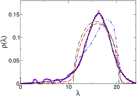
Figure 1. Comparison between the numerically calculated level density (N = 800) for Γ = 1 (red connected symbols) with the SCERM result of Ganter and Schirmacher [1] (blue dash-double dots), our ERM-SCBA result (red dashes) and the half-elliptic DOS (green dash-dots).

In Figure 2 we compare the level density of the numerical simulation with the ERM-SCBA for different values of Γ. The decreasing accuracy of the theoretical results with degreasing Γ might be due to the appearance of finite-size effects (see next paragraph).

FIGURE 2

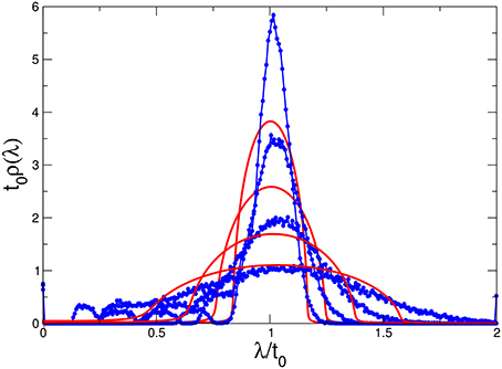
Figure 2. Comparison between the numerically calculated level density (N = 200, blue connected symbols) with the results of ERM-SCBA (red lines) for Γ = 0.3, 0.65, 1.5, and 3.5 (from top to bottom).

We conclude that the ERM-SCBA introduced by us is a handy tool to calculate almost analytically the DOS of a spring-mass model. While the ERM-SCBA is not as accurate as the SCERM theory, it is much easier tractable, because here we have to solve only the SCBA Equation (50c), which requires a few numerical iterations, whereas for the SCERM theory one has to solve the set of three-dimensional integral Equation (19).

3.3. Results for the Moments

3.3.1. The Average 〈f〉 and 〈f²〉 in the Gaussian Case

We are now calculating the averages 〈f〉 and 〈f²〉 needed for the moments. We do this calculation for a finite volume V as present in our numerical calculation.

$\begin{array}{l}\langle f\rangle =\frac{1}{V}{\displaystyle \int d^3}r\exp (-{\overline{r}}^2/2{\sigma }^2)\\ ={\left[\frac{1}{L}{\displaystyle {\int }_{-L/2}^{L/2}d}x\exp (-x^2/2{\sigma }^2)\right]}^3={\left[\sqrt{2\pi }\frac{\sigma }{L}\text{erf}(\frac{\sqrt{2}L}{4\sigma })\right]}^3& (51)\end{array}$

Similarly, 〈f²〉 is obtained by the previous equation with the substitution $\sigma \to \sigma /\sqrt{2}$:

$\begin{array}{ll}\langle f^2\rangle ={\left[\sqrt{\pi }\frac{\sigma }{L}\text{erf}(\frac{L}{2\sigma })\right]}^3& (52)\end{array}$

Summing up:

$\begin{array}{ll}\langle f\rangle ={\left(2\pi \right)}^{3/2}{\left(\frac{\sigma }{L}\right)}^3{\text{erf}}^3(\frac{\sqrt{2}L}{4\sigma })& (53)\end{array}$

$\begin{array}{ll}\langle f^2\rangle ={\pi }^{3/2}{\left(\frac{\sigma }{L}\right)}^3{\text{erf}}^3(\frac{L}{2\sigma })& (54)\end{array}$

In terms of (Γ, N) the averages become:

$\begin{array}{ll}\langle f\rangle =\frac{1}{N}{\left(2\pi \right)}^{3/2}\left(\frac{1}{\Gamma }\right){\text{erf}}^3\left(\frac{\sqrt{2}}{4}{(N\Gamma )}^{1/3}\right)& (55)\end{array}$

$\begin{array}{ll}\langle f^2\rangle =\frac{1}{N}{\pi }^{3/2}\left(\frac{1}{\Gamma }\right){\text{erf}}^3\left(\frac{1}{2}{(N\Gamma )}^{1/3}\right)& (56)\end{array}$

3.3.2. Check at Finite Size

We now compare the exact results for the moments in a finite volume, Equations (9), (11), together with Equations (55), (56) with the results of the numerical simulation as described before.

In the next figures the analytical results are compared, in log log scale, with the simulation for N = 50 and 150. The data are reported as function of Γ in the range 10⁻³–10³. Figure 3 reports the comparison of the analytic calculation (black lines) of the first moment M⁽¹⁾ with the results of the numerical simulation (dots). Similarly, Figure 4 reports the comparison of the analytic calculation of the second moment M⁽²⁾ with the simulation. Finally Figure 5 reports the comparison of the analytic calculation of the second central moments $M_c^{(2)}$ (black) and ${\tilde{M}}_c^{(2)}$ (blue) with the results of the numerical simulation. The red lines in the figure represent the large N (full) and small Γ (dashed) limits. All the comparisons are favorable.

FIGURE 3

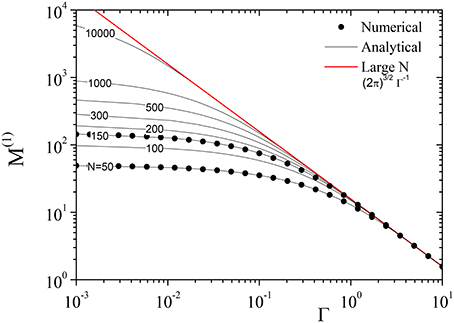
Figure 3. Comparison between the analytical (full lines, from Equations 9 and 55) and numerical (black dots) results for the first moment M⁽¹⁾ of the spectral density of states ρ(λ). λ = ω² are the eigenvalues of the dynamical matrix and ω are the characteristic frequencies. The data at the indicated selected N values are reported as a function of the parameter Γ. The N values (N = 50, 100, 150, 200, 300, 500, 1,000, and 10,000 for the analytical case and 50 and 150 for the numerical one) are indicated on the black curves. The red line is the asymptotic, N→∞, limit reported in Equation (58).

FIGURE 4

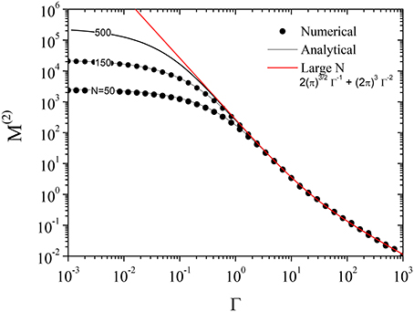
Figure 4. Comparison between the analytical (full lines, from Equations 11, 55, and 56) and numerical (black dots) results for the second moment M⁽²⁾ of the spectral density of states ρ(λ). The data at the indicated selected N values are reported as a function of the parameter Γ. The N values (N = 50, 150, and 500 for the analytical case and 50 and 150 for the numerical one) are indicated on the black curves. The red line is the asymptotic, N→∞, limit reported in Equation (58).

FIGURE 5

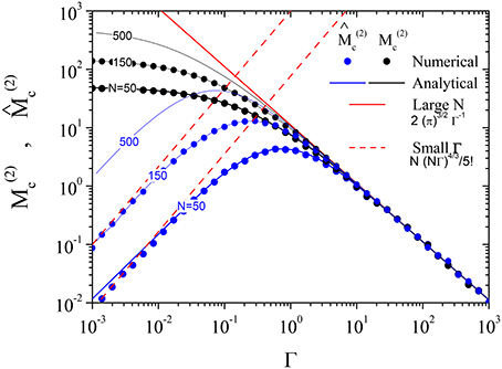
Figure 5. Comparison between the analytical (full lines, from Equations 11, 55, and 56) and numerical (dots) results for the second central moment M⁽²⁾ (black) and for the “non trivial” second central moment ${\tilde{M}}^{(2)}$ (blue) of the spectral density of states ρ(λ). The data at the indicated selected N values are reported as a function of the parameter Γ. The N values (N = 50, 150, and 500 for the analytical case and 50 and 150 for the numerical one) are indicated on the black and blue curves. The red full line is the asymptotic, N→∞, limit reported in Equation (58), it turns out to be the same for M⁽²⁾ and ${\tilde{M}}^{(2)}$. The dashed red lines are the low Γ limit, reported in Equation (60).

3.3.3. Infinite Size Limit

In the limit of infinite size, L→∞, N→∞, ρ = N/L³ = constant, from Equations (55) and (56)

we get (with erf(x) → 1 for large x):

$\begin{array}{ll}\begin{array}{||}\hline N\to \infty \\ \hline\end{array}\begin{array}{l}\{\begin{array}{c}N\langle f\rangle ={(2\pi )}^{3/2}\left(\frac{1}{\Gamma }\right)\\ N\langle f^2\rangle ={\pi }^{3/2}\left(\frac{1}{\Gamma }\right)\end{array}\hfill \end{array}& (57)\end{array}$

Thus, the moments become (in the infinite size limit ${\tilde{M}}^{(n)}=M^{(n)}$):

$\begin{array}{ll}\begin{array}{||}\hline N\to \infty \\ \hline\end{array}\{\begin{array}{l}{M}^{(1)}=\left(\frac{K_o}{M}\right){(2\pi )}^{3/2}\left(\frac{1}{\Gamma }\right)\hfill \\ M^{(2)}={\left(\frac{K_o}{M}\right)}^2\left[2{\pi }^{3/2}\left(\frac{1}{\Gamma }\right)+{(2\pi )}^3\left(\frac{1}{{\Gamma }^2}\right)\right]\hfill \\ M_c^{(2)}={\left(\frac{K_o}{M}\right)}^{2}2{\pi }^{3/2}\left(\frac{1}{\Gamma }\right)\hfill \end{array}& (58)\end{array}$

In the infinite size limit the moments only depend on Γ, which justify the choice of this parameter instead of ρ or/and σ.

These infinite size equations are reported as full red lines in Figures 3–5.

3.3.4. Large and Small Γ Limits

Large Γ is similar to large L, thus the asymptotic expansions in Equation (58) are valid at large Γ with the further simplification that the term in Γ⁻² can be neglected in the expression for M⁽²⁾:

$\begin{array}{ll}\begin{array}{||}\hline \Gamma \to \infty \\ \hline\end{array}\{\begin{array}{l}{M}^{(1)}=\left(\frac{K_o}{M}\right){(2\pi )}^{3/2}\left(\frac{1}{\Gamma }\right)\hfill \\ M^{(2)}={\left(\frac{K_o}{M}\right)}^{2}2{\pi }^{3/2}\left(\frac{1}{\Gamma }\right)\hfill \\ \begin{array}{l}{M}_c^{(2)}={\left(\frac{K_o}{M}\right)}^{2}2{\pi }^{3/2}\left(\frac{1}{\Gamma }\right)\hfill \end{array}\hfill \end{array}& (59)\end{array}$

While straightforward algebra gives the small Γ limit, that turns out to be:

$\begin{array}{ll}\begin{array}{||}\hline \Gamma \to 0\\ \hline\end{array}\{\begin{array}{l}{M}^{(1)}=\left(\frac{K_o}{M}\right)N\hfill \\ M^{(2)}={\left(\frac{K_o}{M}\right)}^2{N}^2\hfill \\ M_c^{(2)}={\left(\frac{K_o}{M}\right)}^{2}N\hfill \\ {\tilde{M}}_c^{(2)}={\left(\frac{K_o}{M}\right)}^2\frac{1}{5!}{N}^{7/3}{\Gamma }^{4/3}\hfill \end{array}& (60)\end{array}$

These limits are easily verified in the three figures previously reported. The equation for ${\tilde{M}}_c^{(2)}$ is reported in Figure 5 as dashed red line.

4. Discussion and Conclusion

In the paper we have shown that the self-consistent euclidean-matrix (SCERM) approximation of Ganter and Schirmacher [1] preserves the two nontrivial moments of the eigenvalue spectrum of mass-and spring models. This confirms the conclusion that the ERM formalism is a very powerful one and is a good starting point for further work.

We have calculated the exact expressions for the 1st and 2nd spectral moments for finite and infinite samples. We show that in the limit of large interaction parameter σ there is a strong size (N) dependence of the spectral moments, thus posing a caveat on the extrapolation of finite-size molecular dynamics simulations to the thermodynamic, large N, limit.

We have established a link between the self-consistent ERM (SCERM) approximation of Ganter and Schirmacher [1] and the self-consistent Born (SCBA) scheme of the heterogeneous-elasticity theory of vibrational anomalies [9, 23]. By this we constructed a simplified version of the SCERM approximation, the ERM-SCBA, which compares well to our numerical diagonalization of the Gaussian-force-constant model. As the SCBA version of herogeneous-elasticity theory has served [9, 23, 47] to explain the vibrational anomalies related to the boson peak this is—in a nutshell—also the case for the new ERM-SCBA.

A more realistic theory, applicable to amorphous solids and liquids in the high-frequency regime should not be based on a scalar mass-spring model but on the full vectorial equations of motions of a disordered solid, interacting via pair potentials. The force constants, which appear in this theory are the second derivatives of the pair potentials. Furthermore the configurational averages should not be based on the random statistics of points but on the statistics of atoms in an amorphous solid, consistent with the pair potentials. Such a theory has been formulated within the ERM scheme by Ciliberti et al. [48], but unfortunately contained a mistake concerning the summation of diagrams, such that the Rayleigh-scattering property was not obtained [1, 49], and the other results are, therefore, questionable. A vectorial version of the ERM-SCBA for the description of amorphous solids will be worked out by the present authors.

Let us mention a drawback of the present approach: The ERM approach is based on an expansion of the averaged Green's function with respect to the inverse density. This means that the theory looses its application range once the density parameter Γ∝ρ⁻¹ becomes much larger than one. In fact, in this regime the spectrum becomes unstable, i.e., negative values of λ are predicted [39, 40, 48]. However, as the force constants K_ij are all positive definite so must be the ensemble of eigenvalues. This artifact can be avoided by using the coherent-potential approximation (CPA) [43] instead of the SCBA. A connection between the ERM and CPA formalism which gives a theory valid for low densities, will be published shortly by the present authors.

Author Contributions

All authors listed, have made substantial, direct and intellectual contribution to the work, and approved it for publication.

Conflict of Interest Statement

The authors declare that the research was conducted in the absence of any commercial or financial relationships that could be construed as a potential conflict of interest.

Footnotes

1. ^In their original papers on the ERM formalism the authors claimed that the model would not exhibit Rayleigh scattering [39, 40]. Ganter and Schirmacher [1] and later Grigera et al. [49] showed that this statement was in error.

References

1. Ganter C, Schirmacher W. Rayleigh scattering, long-time tails, and the harmonic spectrum of topologically disordered systems. Phys Rev B (2010) 82:094205. doi: 10.1103/PhysRevB.82.094205

CrossRef Full Text | Google Scholar

2. Sette F, Krisch MH, Masciovecchio C, Ruocco G, Monaco G. Dynamics of glasses and glass-forming liquids studied by inelastic X-ray scattering. Science (1998) 280:1550–5. doi: 10.1126/science.280.5369.1550

CrossRef Full Text | Google Scholar

3. Binder K, and Kob W. Glassy Materials and Disordered Solids: An Introduction. London: World Scientific (2011).

4. Zeller RC, Pohl RO. Thermal conductivity and specific heat of noncrystalline solids. Phys Rev. B (1971) 4:2029. doi: 10.1103/PhysRevB.4.2029

CrossRef Full Text

5. Shintani H, Tanaka H. Universal link between the boson peak and transverse phonons in glass. Nat Mater (2008) 7:870–7. doi: 10.1038/nmat2293

PubMed Abstract | CrossRef Full Text

6. Horbach J, Kob W, Binder K. High frequency sound and the boson peak in amorphous silica. Eur Phys J B (2001) 19:531–43. doi: 10.1007/s100510170299

CrossRef Full Text

7. Nakayama T. Boson peak and terahertz frequency dynamics of vitreous silica. Rep Prog Phys. (2002) 65:1195. doi: 10.1088/0034-4885/65/8/203

CrossRef Full Text

8. Gurevich VL, Parshin DA, Shober HR. Anharmonicity, vibrational instability, and the Boson peak in glasses. Phys Rev. B (2003) 67:094203. doi: 10.1103/PhysRevB.67.094203

CrossRef Full Text

9. Schirmacher W, Ruocco G, Scopigno T. Acoustic attenuation in glasses and its relation with the boson peak. Phys Rev Lett. (2007) 98:025501. doi: 10.1103/PhysRevLett.98.025501

PubMed Abstract | CrossRef Full Text

10. Rufflé B, Parshin DA, Courtens E, Vacher R. Boson peak and its relation to acoustic attenuation in glasses. Phys Rev Lett. (2008) 100:015501. doi: 10.1103/PhysRevLett.100.015501

PubMed Abstract | CrossRef Full Text

11. Chumakov AI, Monaco G, Monaco A, Crichton WA, Bosak A, Rffer R, et al. Equivalence of the boson peak in glasses to the transverse acoustic van hove singularity in crystals. Phys Rev Lett. (2011) 106:8519. doi: 10.1103/PhysRevLett.106.225501

PubMed Abstract | CrossRef Full Text | Google Scholar

12. Chumakov AI, Monaco G, Fontana A, Bosak A, Hermann RP, Bessas D, et al. Role of disorder in the thermodynamics and atomic dynamics of glasses. Phys Rev Lett. (2014) 112:025502. see also the article of A. L. Chumakov and G. Monaco in this volume. doi: 10.1103/PhysRevLett.112.025502

PubMed Abstract | CrossRef Full Text | Google Scholar

13. Ruocco GF, Sette R, Di Leonardo D, Fioretto M, Lorenzen M, Krisch C, et al. Nondynamic origin of the high-frequency acoustic attenuation in glasses. Phys Rev Lett. (1999) 83:5583. doi: 10.1103/PhysRevLett.83.5583

CrossRef Full Text | Google Scholar

14. Ruocco G, Sette F, Di Leonardo R, Monaco G, Sampoli M, Scopigno T, et al. Relaxation processes in harmonic glasses? Phys Rev Lett. (2000) 84:5788–91. doi: 10.1103/PhysRevLett.84.5788

PubMed Abstract | CrossRef Full Text | Google Scholar

15. Economou EN. Green's Function in Quantum Physics. Heidelberg: Springer-Verlag (1971).

16. Burin AL, Maksimov LA, Polishchuk IY. The phonon transport in crystals with heavy defects. Phys B (1995) 210:49–54. doi: 10.1016/0921-4526(94)00909-F

CrossRef Full Text | Google Scholar

17. Polishchuk IY, Maksimov LA, Burin AL. Localization and propagation of phonons in crystals with heavy impurities. Phys. Reports (1997) 288:205–22. doi: 10.1016/S0370-1573(97)00025-2

CrossRef Full Text | Google Scholar

18. Karpov VG, Klinger I, Ignat'Ev FN. Theory of the low-temperature anomalies in the thermal properties of amorphous structures. Zh Eksp Teor Fiz (1983) 84:760–75.

Google Scholar

19. Buchenau U, Galperin YM, Gurevich VL, Schober HR. Anharmonic potentials and vibrational localization in glasses. Phys Rev B (1991) 43:5039–45. doi: 10.1103/PhysRevB.43.5039

PubMed Abstract | CrossRef Full Text | Google Scholar

20. Buchenau U, Galperin YM, Gurevich VL, Parshin DA, Ramos MA, Schober HR, et al. Interaction of soft modes and sound waves in glasses. Phys. Rev. B (1992) 46:2798. doi: 10.1103/PhysRevB.46.2798

PubMed Abstract | CrossRef Full Text | Google Scholar

21. Gurevich VL, Parshin DA, Schober HR. Pressure dependence of the boson peak in glasses. Phys Rev B (2005) 71:014209. doi: 10.1103/PhysRevB.71.014209

CrossRef Full Text | Google Scholar

22. Maurer E, Schirmacher W. Local oscillators vs. elastic disorder: a comparison of two models for the boson peak. J Low-Temperature Phys. (2004) 137:453–70. doi: 10.1023/B:JOLT.0000049065.04709.3e

CrossRef Full Text | Google Scholar

23. Schirmacher W. Thermal conductivity of glassy materials and the “boson peak. Europhys Lett. (2006) 73:892. doi: 10.1209/epl/i2005-10471-9

CrossRef Full Text | Google Scholar

24. Schirmacher W, Schmid B, Tomaras C, Viliani G, Baldi G, Ruocco G. Vibrational excitations in systems with correlated disorder. Phys Status Solidi (c) (2008) 5:862. doi: 10.1002/pssc.200777584

CrossRef Full Text | Google Scholar

25. Schirmacher W, Schmid B, Tomaras C, Baldi G, Viliani G, Ruocco G, et al. Sound attenuation and anharmonic damping in solids with correlated disorder. Condensed Mater Phys. (2010) 13:23606. doi: 10.5488/CMP.13.23606

CrossRef Full Text | Google Scholar

26. Tomaras C, Schirmacher W. High-frequency vibrational density of states of a disordered solid. J Phys Condens Matter (2013) 25:495402. doi: 10.1088/0953-8984/25/49/495402

PubMed Abstract | CrossRef Full Text | Google Scholar

27. Schirmacher W. The boson peak. Phys Stat Sol. (b) (2013) 250:937. doi: 10.1002/pssb.201248544

CrossRef Full Text | Google Scholar

28. Schirmacher W, Scopigno T, Ruocco G. Theory of vibrational anomalies in glasses. J Noncryst Sol. (2014) 407:133–40. doi: 10.1016/j.jnoncrysol.2014.09.054

CrossRef Full Text | Google Scholar

29. Schirmacher W, Wagener M. In: Dianoux AJ, Petry W, Teixeira J, editors. Dynamics of Disordered Materials. Heidelberg: Springer (1989).

30. Xu BC, Stratt RM. Liquid theory for band structure in a liquid. II. P orbitals and phonons. J Chem Phys. (1990) 92:1923. doi: 10.1063/1.458023

CrossRef Full Text

31. Wu TM, Loring RF. Phonons in liquids: a random walk approach. J Chem Phys. (1990) 97:8568. doi: 10.1063/1.463375

CrossRef Full Text

32. Schirmacher W, Wagener M. Analogies between hopping and phonon propagation in disordered solids. Philos Magn B (1992) 65:861. doi: 10.1080/13642819208204892

CrossRef Full Text

33. Schirmacher W, Wagener M. Vibrational anomalies and phonon localization in glasses. Sol State Comm. (1993) 86:597–603. doi: 10.1016/0038-1098(93)90147-F

CrossRef Full Text

34. Kühn R, Horstmann U. Random matrix approach to glassy physics: low temperatures and beyond. Phys Rev Lett. (1997) 78:4067. doi: 10.1103/PhysRevLett.78.4067

CrossRef Full Text

35. Schirmacher W, Diezemann G, Ganter C. Harmonic vibrational excitations in disordered solids and the “boson peak”. Phys Rev Lett. (1998) 81:136. doi: 10.1103/PhysRevLett.81.136

CrossRef Full Text

36. Schirmacher W, Diezemann G, Ganter C. Model calculations for the vibrational anomalies of a disordered Lennard Jones solid. Phys B (2000) 284–288:1147. doi: 10.1016/S0921-4526(99)02550-8

CrossRef Full Text

37. Martín-Mayor V, Parisi G, Veroccio P. Dynamical structure factor in disordered systems. Phys Rev E (2000) 62:2373. doi: 10.1103/PhysRevE.62.2373

PubMed Abstract | CrossRef Full Text

38. Taraskin SN, Elliott S, Loh YH, Nataranjan G. Origin of the boson peak in systems with lattice disorder. Phys Ref Lett. (2001) 86:1255–8. doi: 10.1103/PhysRevLett.86.1255

PubMed Abstract | CrossRef Full Text

39. Grigera TS, Martin-Mayor V, Parisi G. Verrocchio P. Vibrational spectrum of topologically disordered systems. Phys Rev Lett. (2001) 87:085502. doi: 10.1103/PhysRevLett.87.085502

CrossRef Full Text

40. Martín-Mayor V, Mzard M, Parisi G, Verrocchio P. The dynamical structure factor in topologically disordered systems. J Chem Phys. (2001) 114:8068. doi: 10.1063/1.1349709

CrossRef Full Text

41. Grigera TS, Martín-Mayor V, Parisi G, Verrocchio P. Phonon interpretation of the ‘boson peak’ in supercooled liquids. Nature (2003) 422:289–92. doi: 10.1038/nature01475

PubMed Abstract | CrossRef Full Text

42. Amir A, Krich JJ, Vitelli V, Oreg Y, Imry Y. Emergent percolation length and localization in random elastic networks. Phys Rev X (2013) 3:021017. doi: 10.1103/PhysRevX.3.021017

CrossRef Full Text

43. Köhler S, Ruocco R, Schirmacher W. Coherent potential approximation for diffusion and wave propagation in topologically disordered systems. Phys Rev B (2013) 88:064203. doi: 10.1103/PhysRevB.88.064203

CrossRef Full Text

44. Hubbard J, Beeby JL. Collective motion in liquids. J Phys C (Solid St. Phys.) (1969) 2:556.

45. Golub GH, van der Vorst A. Eigenvalue computation in the 20th century. J Comput Appl Math. (2000) 123:35–65. doi: 10.1016/S0377-0427(00)00413-1

CrossRef Full Text

46. Elliott SR. Handbook of Mathematical Functions. New York, NY: Wiley–Interscience (1973).

47. Marruzzo A, Schirmacher W, Fratalocchi A, Ruocco G. Heterogeneous shear elasticity of glasses: the origin of the boson peak. Nat Sci Rep. (2013) 3:1407. doi: 10.1038/srep01407

PubMed Abstract | CrossRef Full Text

48. Ciliberti S, Grigera TS, Martin-Mayor V, Parisi G, Verrocchio P. Brillouin and boson peaks in glasses from vector Euclidean random matrix theory. J Chem Phys. (2003) 119:8577. doi: 10.1063/1.1610439

CrossRef Full Text

49. Grigera TS, Martín-Mayor V, Parisi G, Urbani P, Verrocchio P. On the high-density expansion for Euclidean random matrices. J Stat Mech. (2011) 2011:P02015. doi: 10.1088/1742-5468/2011/02/P02015

CrossRef Full Text

A. Appendix

A.1. Detailed Calculation of the Moments

A.1.1. First Moment

From Equation (7) the first (n = 1) moment is given by the trace of the dynamical matrix:

$\begin{array}{l}{M}^{(1)}=\frac{1}{N}\langle tr\left\{D\right\}\rangle =\frac{1}{N}\text{}\langle {\displaystyle \sum _i\text{}}{D}_{ii}\text{}\rangle \\ =-\frac{1}{N}\langle {\displaystyle \sum _{i,j\ne i}{D}_{ij}}\rangle =\frac{K_0}{MN}{\displaystyle \sum _{i,j\ne i}\langle f_{ij}\rangle }& (\text{A}1)\end{array}$

The sum appearing in the rightmost term in this equation is extended over N(N − 1) terms, all different each others, thus statistically independent, and all arising from the same probability distribution function ${P}$(f). Therefore we can write:

$\begin{array}{ll}{M}^{(1)}=\frac{K_0}{M}(N-1)\langle f\rangle & (\text{A}2)\end{array}$

The whole set of first moments, according to their definition, turn out to be:

$\begin{array}{l}{M}^{(1)}=\frac{K_0}{M}(N-1)\langle f\rangle \\ M_c^{(1)}=0\\ {\tilde{M}}^{(1)}=\frac{K_0}{M}N\langle f\rangle \\ {\tilde{M}}_c^{(1)}=0& (\text{A}3)\end{array}$

A.1.2. Second Moment

Following the same steps as in the case of the first moment, we have:

$\begin{array}{l}{M}^{(2)}=\frac{1}{N}\langle \text{tr}\left\{D^2\right\}\rangle =\frac{1}{N}\langle {\displaystyle \sum _{ij}{D}_{ij}}{D}_{ji}\rangle =\frac{1}{N}\langle {\displaystyle \sum _{ij}{D}_{ij}^2}\rangle =\\ {\left(\frac{K_0}{M}\right)}^2\frac{1}{N}\langle {\displaystyle \sum _{i,j}{\left\{\left[{\displaystyle \sum _{k\ne i}{f}_{ik}}\right]{\delta }_{ij}-f_{ij}(1-{\delta }_{ij})\right\}}^2}\rangle \end{array}$

Expanding the square in the sum of the rightmost term in the previous equation, keeping in ind that ${\delta }_{ij}^2={\delta }_{ij}$, ${(1-{\delta }_{ij})}^2=1-{\delta }_{ij}$, δ_ij(1 − δ_ij) = 0):

$\begin{array}{l}{M}^{(2)}={\left(\frac{K_0}{M}\right)}^2\frac{1}{N}{\displaystyle \sum _{i,j}\langle {\left[{\displaystyle \sum _{k\ne i}{f}_{ik}}\right]}^2{\delta }_{ij}+f_{ij}^2(1-{\delta }_{ij})\rangle }\end{array}$

thus

$\begin{array}{l}{M}^{(2)}={\left(\frac{K_0}{M}\right)}^2\frac{1}{N}\langle {\displaystyle \sum _{i,j}{\left[{\displaystyle \sum _{k\ne i}{f}_{ik}}\right]}^2}{\delta }_{ij}+{\displaystyle \sum _{i,j}{f}_{ij}^2}(1-{\delta }_{ij})\rangle \\ ={\left(\frac{K_0}{M}\right)}^2\frac{1}{N}\langle {\displaystyle \sum _i{\left[{\displaystyle \sum _{k\ne i}{f}_{ik}}\right]}^2}+{\displaystyle \sum _{i,j\ne i}{f}_{ij}^2}\rangle \\ ={\left(\frac{K_0}{M}\right)}^2\text{}\frac{1}{N}\langle {\displaystyle \sum _i{\left[{\displaystyle \sum _{k\ne i}{f}_{ik}}\right]}^2}+{\left(\frac{K_0}{M}\right)}^2\frac{1}{N}{\displaystyle \sum _{i,j\ne i}{f}_{ij}^2}\rangle \\ ={\left(\frac{K_0}{M}\right)}^2\text{}\frac{1}{N}\langle {\displaystyle \sum _i\left[{\displaystyle \sum _{k\ne i}{\displaystyle \sum _{k^{\prime }\ne i}{f}_{ik}}}{f}_{ik\prime }\right]}+{\displaystyle \sum _{i,j\ne i}{f}_{ij}^2}\rangle \end{array}$

In the first sum of the latter expression there are N(N − 1) terms $f_{ik}^2$ (arising from k = k′ ≠ i) and N(N − 1)(N − 2) terms $f_{ik}{f}_{i{k}^{\prime }}$ with all the three indexes i, k, k′ different each others. In the second summation there are N(N − 1) terms $f_{ij}^2$ (i ≠ j). Therefore:

$\begin{array}{l}{M}^{(2)}=\text{}{\left(\frac{K_0}{M}\right)}^2\text{}\frac{1}{N}\text{}\left[N(N\text{}-\text{}1)\langle f^2\rangle +N(N\text{}-\text{}1)(N\text{}-\text{}2){\langle f\rangle }^2\right]\\ +{\left(\frac{K_0}{M}\right)}^2\frac{1}{N}N(N-1)\langle f^2\rangle \end{array}$

with, similar to before:

$\begin{array}{ll}\langle f^2\rangle \doteq \frac{1}{N(N-1)}{\displaystyle \sum _{i,j\ne i}}\langle f_{ij}^2\rangle & (\text{A}4)\end{array}$

Overall:

$\begin{array}{ll}{M}^{(2)}={\left(\frac{K_0}{M}\right)}^2\left[2(N-1)\langle f^2\rangle +(N-1)(N-2){\langle f\rangle }^2\right]& (\text{A}5)\end{array}$

Now $M_c^{(2)}$can be easily obtained:

$\begin{array}{ll}{M}_c^{(2)}={\left(\frac{K_0}{M}\right)}^2(N-1)\left[2\langle f^2\rangle -{\langle f\rangle }^2\right]& (\text{A}6)\end{array}$

Then

$\begin{array}{ll}{\widehat{M}}^{(2)}={\left(\frac{K_0}{M}\right)}^2\left[2N\langle f^2\rangle +N(N-2){\langle f\rangle }^2\right]& (\text{A}7)\end{array}$

and

$\begin{array}{ll}{\tilde{M}}_c^{(2)}=2N{\left(\frac{K_0}{M}\right)}^2\left[\langle f^2\rangle -{\langle f\rangle }^2\right]& (\text{A}8)\end{array}$

Summing up the different second moments (by neglecting terms of order 1 with respect to N):

$\begin{array}{l}{M}^{(2)}={\left(\frac{K_0}{M}\right)}^2\left[2N\langle f^2\rangle +N^2{\langle f\rangle }^2\right]\\ M_c^{(2)}={\left(\frac{K_0}{M}\right)}^{2}N\left[2\langle f^2\rangle -{\langle f\rangle }^2\right]\\ {\widehat{M}}^{(2)}={\left(\frac{K_0}{M}\right)}^2\left[2N\langle f^2\rangle +N^2{\langle f\rangle }^2\right]\\ {\widehat{M}}_c^{(2)}={\left(\frac{K_0}{M}\right)}^{2}2N\left[\langle f^2\rangle -{\langle f\rangle }^2\right]& (\text{A}9)\end{array}$